The document discusses the acceleration of global warming since 2010, which has increased by over 50% compared to the previous decades, contributing to Earth's warming beyond stable levels seen in the Holocene. It examines human-made greenhouse gases and aerosols as primary factors driving this change, highlighting that the perceived cooling effect of aerosols offsets the warming from greenhouse gases, leading to underestimated climate sensitivity and heightened future risks. The authors argue for a better understanding of climate forcing mechanisms and their implications on climate policy and public awareness.

1. Environment: Science and Policy for Sustainable
Development
ISSN: (Print) (Online) Journal homepage: www.tandfonline.com/journals/venv20
Global Warming Has Accelerated: Are the United
Nations and the Public Well-Informed?
James E. Hansen, Pushker Kharecha, Makiko Sato, George Tselioudis, Joseph
Kelly, Susanne E. Bauer, Reto Ruedy, Eunbi Jeong, Qinjian Jin, Eric Rignot,
Isabella Velicogna, Mark R. Schoeberl, Karina von Schuckmann, Joshua
Amponsem, Junji Cao, Anton Keskinen, Jing Li & Anni Pokela
To cite this article: James E. Hansen, Pushker Kharecha, Makiko Sato, George Tselioudis,
Joseph Kelly, Susanne E. Bauer, Reto Ruedy, Eunbi Jeong, Qinjian Jin, Eric Rignot, Isabella
Velicogna, Mark R. Schoeberl, Karina von Schuckmann, Joshua Amponsem, Junji Cao, Anton
Keskinen, Jing Li & Anni Pokela (2025) Global Warming Has Accelerated: Are the United Nations
and the Public Well-Informed?, Environment: Science and Policy for Sustainable Development,
67:1, 6-44, DOI: 10.1080/00139157.2025.2434494
To link to this article: https://doi.org/10.1080/00139157.2025.2434494
© 2025 The Author(s). Published with
license by Taylor & Francis Group, LLC
View supplementary material
Published online: 03 Feb 2025.
Submit your article to this journal
View related articles
View Crossmark data
Full Terms & Conditions of access and use can be found at
https://www.tandfonline.com/action/journalInformation?journalCode=venv20

2. 6 ENVIRONMENT WWW.TANDFONLINE.COM/VENV VOLUME 67 NUMBER 1
by James E. Hansen, Pushker Kharecha, Makiko Sato,
George Tselioudis, Joseph Kelly, Susanne E. Bauer, Reto Ruedy,
Eunbi Jeong, Qinjian Jin, Eric Rignot, Isabella Velicogna,
Mark R. Schoeberl, Karina von Schuckmann, Joshua Amponsem,
Junji Cao, Anton Keskinen, Jing Li, and Anni Pokela
iStock/Annadokaz

3. ENVIRONMENT 7
JANUARY/FEBRUARY 2025 WWW.TANDFONLINE.COM/VENV
G
lobal warming has
accelerated since 2010 by
more than 50% over the
1970-2010 warming rate
of 0.18°C per decade1
(Figure 1).2
Earth is now warmer than at
any time in the Holocene, the past 11,700
years of relatively stable climate in which
civilization developed, and it is at least as
warm as during the extreme warm
Eemian interglacial period 120,000 years
ago. Global temperature increased 0.4°C
during the recent moderate El Niño (a
period when east-to-west equatorial trade
winds weaken, allowing warm waters of
the West Pacific to move toward South
America), a warming much greater than
during even the strongest prior El Niños.
This rapid warming has baffled leading
Earthscientists,who,forexample,conclude
thatnocombinationofknownmechanisms
forwarming“hasbeenabletoreconcileour
theories with what has happened.”3
We
conclude, on the contrary, that the known
drives for climate change, principally
human-madegreenhousegasesandaerosols,
account for observed global temperature,
includingajumpinseasurfacetemperature
thatamplifiedwarmingduringtheElNiño
and has caused the widely discussed 1.5°C
temperature threshold to be breached, for
all practical purposes.
Climate change burst into public atten-
tion with climate anomalies in 1988 so
extreme that Time Magazine declared
Earthtobe“personoftheyear.”Risingpub-
licinterestinclimatechange,especiallythe
role of humanity in causing change, led to
the 1992 United Nations Framework
Convention on Climate Change4
and a
largeincreaseinfundingforclimateobser-
vations and research. The Framework
Convention aimed to prevent dangerous
human-causedclimatechange.Thelargest
fundingincreasewasforaNASAprogram
initially titled Mission to Planet Earth
expected to make global observations
needed to understand ongoing global
change.
By 1992 it was understood that two
things caused large human effects on cli-
mate: greenhouse gases (GHGs) and aero-
sols (tiny, generally microscopic, particles
suspended in the air). GHGs cause global
warming by holding in Earth’s heat radia-
tion, acting like a blanket. The physics of
this greenhouse effect is well understood
and tested, for example, by comparison of
Mars,EarthandVenus,withtheirdiffering
amounts of atmospheric GHGs. Carbon
dioxide (CO2), produced mainly by burn-
ingoffossilfuels(coal,oilandgas)butalso
by deforestation, causes more than half of
the human-made greenhouse warming.
Human-made increases of CO2 and the
other main GHGs (Sidebar 2) have long
lifetimes in the atmosphere from decades
to millennia. Thus, these gases are well-
mixed in the atmosphere and it is easy to
measure their changing global amounts.
Human-made aerosols with greatest
effect on climate are products of fossil
fuel burning and biofuels (like firewood).
Most aerosols increase reflection of
incoming sunlight back to space and thus
have a global cooling effect. Charlson and
colleagues5
concluded in 1992 that the
climate forcing by aerosols – the cooling
drive for climate change, see below – was
similar in magnitude to the GHG forcing,
but opposite in sign, thus tending to off-
set GHG warming. Aerosol offset of GHG
warming is a Faustian bargain (Figure 2),6
that is, a bargain providing present benefit
withoutregardtofutureconsequences.The
aerosols providing a cooling benefit are
also inherently dangerous particulate air
pollutionresponsibletodayforseveralmil-
lion annual deaths by respiratory, cardio-
vascular, and even neurological diseases
worldwide;7
thus,asglobalpollutioncontrol
has improved and clean energies are intro-
duced the cooling effect of aerosols is lost:
withthechangeofshipregulations,ourfirst
Faustian payment came due.1,8
Climate sensitivity is a measure of the
effect of rising levels of greenhouse gases
on Earth’s temperature. It is usually
defined as the eventual increase of global
average temperature after a doubling of
CO2 concentration in the atmosphere
compared to pre-industrial levels.
In this paper, we conclude that the esti-
mate of aerosol climate forcing (Figure 3)
by the United Nation’s scientific advisory
body (the Intergovernmental Panel on
Climate Change, IPCC) is an underesti-
mate, and thus the Faustian bargain is
worse than expected. We also show that
IPCC’semphasisonglobalclimatemodels
led to a marriage of aerosol forcing and
climatesensitivity,suchthatunderestimate
of aerosol forcing led to underestimate of
climate sensitivity. The result is a double
whammy that helps explain global warm-
ing acceleration and alters projections of
future climate, magnifying the danger of
Figure 1. Global surface temperature change
(see Sidebar 1).
Sidebar 1. Global surface
temperature relative to
1880-1920 in Figure 1 is the
GISS (Goddard Institute
for Space Studies) analysis
through October 2024.2
The
1970-2010 warming rate
of 0.18°C/decade almost
doubled in 2010-2023, but
this higher rate is not a
prediction of the future. A
downturn in greenhouse
gas emissions could alter
projections on decadal time
scales.

4. 8 ENVIRONMENT WWW.TANDFONLINE.COM/VENV VOLUME 67 NUMBER 1
intergenerational injustice. The delayed
response of climate still allows a potential
bright future for today’s young people, but
that happy result requires understanding
of the factors driving climate change.
Theseissuescanbereadilyunderstoodvia
the most basic concepts, beginning with
climate forcings.
Climate Forcings
Climate forcings are imposed changes
of Earth’s energy balance. If the Sun
suddenly became 1% brighter, for exam-
ple, that would be a forcing of +2.4 W/m2
(W/m2
is watts, a measure of energy
transfer over time, per square meter)
becauseEarthnormallyabsorbs240W/m2
of solar energy averaged over Earth’s
surface. Solar variability is one of the
two natural climate forcings that are
important on time scales of years to cen-
turies, the other being large volcanic
eruptions that inject gases and aerosols
into Earth’s stratosphere (at about 15-50
kilometers, 10-30 miles). It is helpful to
compare these well-understood natural
forcings with human-made climate
forcings.
Our Sun is a rather quiescent star, in
the family of all stars, yet the variability
of dark areas (sunspots) on the solar sur-
face has long caused suspicion that the
Sun may drive climate change on Earth.
Fortunately, NASA has done a good job
of monitoring the solar energy received
at Earth since the late 1970s. Variations
of the Sun’s brightness during the solar
sunspot cycle are about 0.1% (Figure 4),
a forcing change of about 0.25 W/m2
between solar minimum and solar max-
imum outputs. This solar forcing, we will
show, is much smaller than human-made
forcings, but large enough to be a partial
cause of present climate extremes.
Volcanic eruptions produce occasional
large climate forcings. When Mount
Pinatubo erupted in the Philippines in
1991, producing the greatest climate forc-
ing of the 20th century, NASA had satel-
lites in orbit that provided a precise test of
aerosolforcing.SAGE(stratosphericaero-
sol and gas experiment) measurements
Figure 2. Faustus contemplates bargain with Mephistopheles, who offers him his
present desire at the cost of future detriment, much like the cooling benefit of
aerosols, which extract a cost in rapidly increased global warming once society
no longer tolerates unhealthy air pollution.8
Figure 3. Greenhouse gas and IPCC aerosol forcings
(Sidebar 2).**

5. ENVIRONMENT 9
JANUARY/FEBRUARY 2025 WWW.TANDFONLINE.COM/VENV
yielded the average aerosol size and the
dispersion of aerosol sizes.
ERBE (Earth radiation budget
experiment) measured the change of
Earth’s energy balance, which peaked
at −3 W/m2
cooling several months
after the eruption, the delay due to the
time for conversion of the volcanic SO2
gas into atmospheric sulfuric acid aero-
sols and the time for stratospheric
winds to disperse the aerosols around
much of the world. Observed global
cooling after the Pinatubo eruption
peaked at about 0.3 °C, consistent with
expectations given the ocean’s thermal
inertia and the brevity of forcing
(stratospheric circulation carries aero-
sols to polar latitudes where they
descend and are washed from the
atmosphere).
A huge submarine volcanic eruption
on 15 January 2022 – Hunga in the
Pacific Ocean, east of Australia, near the
dateline – blasted about 150 million tons
of water vapor and 1 million tons of SO2
into Earth’s stratosphere. It was much less
SO2 than for Pinatubo, and any cooling
effect was partly offset by warming from
the added stratospheric water vapor (a
GHG).16
Nevertheless, we need to esti-
mate the possible effect of Hunga on
global temperature in 2022-2023 to see if
it had a significant effect on the unprec-
edentedwarmingthatfollowed.Although
it is difficult to disentangle Hunga effect
on Earth’s measured energy balance from
natural variability (due mainly to cloud
variability), analysis shows that aerosol
cooling dominated over water vapor
warming16
and the net volcanic forcing
declined to a small fraction of its peak
value by two years after the eruption. We
approximate the Hunga forcing based on
the Pinatubo forcing (Figure 5), but with
Sidebar 2. Contributions of different greenhouse gases (GHGs) to the
increase of GHG climate forcing since 1750 and in the 10 years 2014-
2023. CH4 forcing includes the effect of increasing stratospheric water
vapor and the portion of O3 change caused by CH4 change.1
MPTGs
are Montreal Protocol Trace Gases and OTGs are Other Trace Gases.
N2O is nitrous oxide, which is increasing from applying nitrogen
fertilizers and from animal waste. Forcings are calculated from
published formulae1
and other graphs of the forcings are available.9
Figure S2. Contribution to greenhouse
gas climate forcing (%).**
Figure 4. Solar irradiance (top) and sunspot numbers.10

6. 10 ENVIRONMENT WWW.TANDFONLINE.COM/VENV VOLUME 67 NUMBER 1
Figure 5. Observed and simulated forcing by Pinatubo aerosols (see also Sidebar 3).**
Sidebar 3. SO2 injected into the stratosphere by volcanoes forms sulfuric acid aerosols over time that are carried
toward the poles and downward by atmospheric circulation and gravity, largely removed in 1-2 years. The large
1991 Pinatubo eruption allows the aerosol forcing to be defined and provide a test of climate impact. Prediction11
of global cooling by Pinatubo aerosols was made soon after the eruption based on initial estimates of aerosol
amount, with peak aerosol forcing −4.5 W/m2
and predicted global cooling 0.5°C. Later multispectral aerosol
opacity data of the SAGE satellite instrument12
allowed precise evaluation of opacity of the Pinatubo aerosol layer
and the dispersion of aerosol sizes,13
which revealed peak forcing as actually −3 W/m2
. Multiple runs of a GCM
(global climate model) with this aerosol forcing produced maximum global cooling after the volcano of 0.3°C and
a maximum decrease of Earth’s energy balance of 3 W/m2
(Figure 5) consistent with ERBE satellite observations.14
SO2 injected into the stratosphere by Hunga is estimated as 1±0.5 megatons,15
an order of magnitude less than
Pinatubo’s 20 megatons. We reduced Pinatubo forcing accordingly and smoothed the Pinatubo forcing curve14
with a 3-month running-mean to obtain our estimate of the Hunga forcing. Later estimates (NASA and USask)16,17
based on satellite data bracket the estimate based on Pinatubo but have earlier peak opacity, likely due to the higher
latitude of the Hunga eruption, which placed the aerosols closer to where they descend from the stratosphere.
Figure S3. Hunga aerosol forcing.**

7. ENVIRONMENT 11
JANUARY/FEBRUARY 2025 WWW.TANDFONLINE.COM/VENV
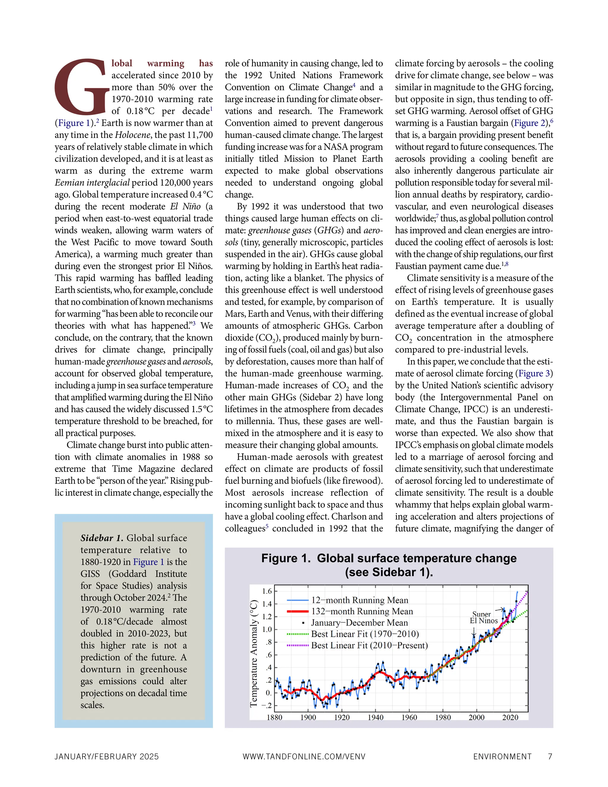
peak forcing −0.3 W/m2
. Like the solar
forcing, the Hunga forcing is small.
Given that we know precisely the nat-
ural climate forcings – volcanic aerosols
and solar irradiance – as well as the
human-made and natural greenhouse gas
forcings, it is obvious that human-made
aerosol forcing is the elephant in the cli-
mate forcing story that receives too little
attention. Aerosol forcing occurs in part
from the direct effect of human-made
aerosols as they reflect and absorb
incoming sunlight, but also from the
indirect aerosol effect as the added aero-
sols modify cloud properties as discussed
below. IPCC estimates the indirect aero-
sol forcing based largely on mathematical
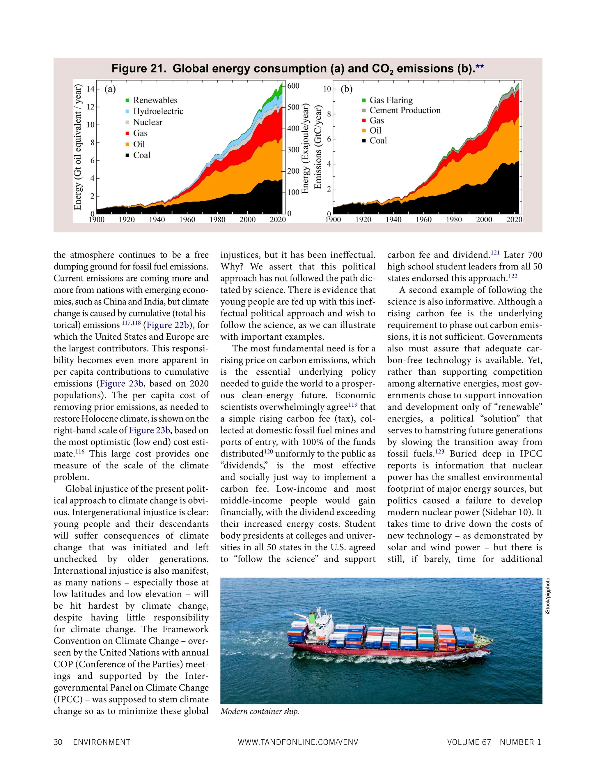
models.18
We suggest that this modeling
fails to fully capture the fact that human-
made aerosols have a larger impact on
clouds when the aerosols are injected into
relatively pristine air in places that are
susceptible to cloud changes. Later in this
paper, we use spatial and temporal
changes of climate and Earth’s energy
balance to explore this indirect aerosol
forcing. First, however, we discuss aero-
sol and cloud particle microphysics.
Aerosol and Cloud Particle
Microphysics
Climate forcing by aerosols depends
on aerosol and cloud processes on min-
ute scales. Aerosol composition matters,
both for the direct effect of aerosols on
radiation and the indirect effect on
clouds. Indirect aerosol forcing arises
because aerosols are condensation nuclei
(tiny sites of water vapor condensation
or “cloud seeds”) for cloud drops. More
nuclei yield more cloud particles and
brighter clouds that reflect more sunlight
and cause cooling.19
More aerosols also
increase cloud cover, as shown by cloud
trails behind ships (“ship tracks”).20
Observations to quantify these effects are
challenging because human-made aero-
sols must be distinguished from changes
of natural aerosols. Thus, there is large
uncertainty in the overall net aerosol
forcing.21,22
Simultaneous with human-caused
aerosol and cloud changes, clouds also
change as a climate feedback. [Climate
feedbacks – response of the climate sys-
tem (such as change of clouds or sea ice)
to climate change – can be either ampli-
fying or diminishing. Amplifying feed-
backs increase climate change, tending to
produce instability, while diminishing
feedbacks decrease climate change, pro-
moting stability.] Cloud feedback is the
main cause of uncertainty in climate sen-
sitivity,theholygrailofclimateresearch.23
Climate sensitivity is defined as global
temperature response to a standard forc-
ing. Observations reveal that the sizes
and locations of zones with different
characteristic clouds are changing – the
intertropical convergence zone (encir-
cling the Earth near the thermal equator)
is shrinking, the subtropics are expand-
ing, and the midlatitude storm zone (not
near the poles or the equator) is shifting
poleward24
– with associated changes of
Earth’s energy balance that constitute
potentially powerful, but still inade-
quately understood, climate feedbacks.
Some of the difficulties in climate mod-
eling include cloud microphysics, such as
the need to realistically simulate mixed
phase (both ice and water) clouds.25
As
cloud modeling has become more com-
plex and realistic, several global climate
models have found higher climate sensi-
tivity correlated with more realistic cloud
distributions (Sidebar 4).
Given the importance of aerosol cli-
mate forcing and climate sensitivity,28
there is a crying need for global monitor-
ing of aerosol and cloud particle micro-
physics and cloud macrophysics29
to help
sort out climate forcings and feedbacks.30
Global monitoring of aerosol/cloud
microphysical properties and cloud mac-
rophysics from a dedicated small satellite
mission has been proposed, but not
implemented.31
The need for such data
will only increase in coming decades as
the world recognizes growing conse-
quences of climate change and tries to
chart a course to restore Holocene-level
global climate. NASA’s 2024PACE satel-
lite mission32
includes polarimeters capa-
ble of measuring aerosol and cloud
microphysics including aerosol and
cloud droplet number concentrations,
which could be a step toward a dedicated,
long-term aerosol mission to monitor
global aerosol and cloud properties as
required to calculate climate forcings and
feedbacks33
(analogous to greenhouse gas
monitoring that permits calculation of
greenhouse gas forcing). In the absence
of that data, we now explore less direct
evidence of aerosol climate forcing.
Evidence of Aerosol Climate
Forcing
Paleoclimate data suggest the import-
ant role of aerosols in global climate. In
the past 6,000 years, known as the late
Holocene, atmospheric CO2 and CH4
increased markedly, likely as a result of
deforestation and methane from rice
agriculture,34
causing greenhouse gas
(GHG) climate forcing to increase more
than 0.5 W/m2
,1
yet global temperature
during the late Holocene held steady35
or
decreased slightly.36
This divergence of
GHG forcing and global temperature is
a strong anomaly; CO2 is a tight control
knob on global temperature at other
times in the ancient paleo record (see
Figure 2 in Note 1 at end), as anticipated
on theoretical grounds.37
Aerosols, the
other large human-made climate forcing,
isasuggestedsolution38
forthis“Holocene
conundrum.” Aerosols increased in recent
millennia as burning of wood and other
biofuels provided fuel for a growing
global population. Moving to recent, pre-
industrial, times, the required magnitude
of the implied (negative) aerosol forcing
from biofuel burning reached at least 0.5
W/m2
. Biofuel aerosol forcing has likely
increased since then, as the biofuel energy
source is widespread in developing
countries and continues in developed
countries.1
Recent restrictions on ship emissions
provide a great opportunity to investi-
gate aerosol forcing. The International
Maritime Organization (IMO) intro-
duced limits on the sulfur content of ship
fuels in stages, with the greatest global
restriction effective January 2020
(Sidebar 5). Change of global aerosol
forcing from this limit on ship emissions,
based on IPCC’s formulation of aerosol
forcing,18
is calculated39
as 0.079 W/m2
.
Forster et al.,40
updating IPCC’s aerosol
forcing, estimate the ship aerosol forcing
change as +0.09 W/m2
; they also note

8. 12 ENVIRONMENT WWW.TANDFONLINE.COM/VENV VOLUME 67 NUMBER 1
Sidebar 4. CMIP (Climate Model Intercomparison Project) studies are carried out prior to and in conjunction
with IPCC reports, with corresponding numbering. Zelinka et al. (2021)50
show that increased equilibrium
climate sensitivity (ECS) of CMIP6 models is primarily due to differences in simulated shortwave (shortwave
refers to solar radiation, as opposed to longwave terrestrial heat radiation) low-cloud feedbacks at middle
and high latitudes in the Southern Hemisphere (Figure S4a). CMIP6 models have a stronger positive low-
cloud feedback at midlatitudes in the Southern Hemisphere and a weaker negative low-cloud feedback at
high latitudes; both features contribute to higher ECS in many CMIP6 models and in the average of all
CMIP6 models.
Jiang et al. (2023)26
show that CMIP6 models with higher ECS produce a realistic seasonal cycle of
extratropical low clouds with peaks in the austral (southern hemisphere) and boreal (northern hemisphere)
winter seasons, while models with lower ECS produce low-cloud seasonal cycles with unrealistic peaks in
summer (Figure S4b). The greater skill of high ECS models in simulating cloud variability and cloud feedbacks,
especially in the Southern Ocean region, suggests greater confidence in the higher ECS models. Cloud changes
are the cause of higher sensitivity in high-ECS models, and thus the observed cloud seasonality provides
significant support for high ECS.
Finally, Williams et al. (2020)27
tested two alternative cloud configurations in the UK Met Office Unified Model
used for weather predictions, finding that the more recent cloud parameterization scheme increases simulated
ECS by 2.2°C, improves the short-range weather forecast, and reduces the error growth over the first few hours of
the forecast, indicative of more realistic modeling of local physical processes. These several works indicate that
high ECS models are more skillful in simulating cloud feedbacks, a crucial factor in determining real-world ECS.
Figure S4a. Shortwave low cloud feedbacks (W/m2
per °C).**
Figure S4b. Shortwave low cloud feedbacks (W/m2
per °C).**

9. ENVIRONMENT 13
JANUARY/FEBRUARY 2025 WWW.TANDFONLINE.COM/VENV
that this ship aerosol forcing would be
offset by negative aerosol forcing from
increased forest fires and other biomass
burning. A review41
of five ship aerosol
modeling studies finds a range 0.07 to
0.15 W/m2
, with mean 0.12±0.03 W/m2
.
A recent model result42
of 0.2 W/m2
refers to ocean area and is thus a global
forcing of 0.14 W/m2
. None of these
modeled Ship Aerosol Forcings would
have much effect on global temperature
because GHG forcing currently is
increasing 0.4-0.5 W/m2
per decade.
However, if the aerosol effect is highly
nonlinear (i.e., if aerosols emitted into
polluted air have much less effect on
clouds than aerosols emitted into a pris-
tine atmosphere), decreased ship emis-
sions may have a large effect on Earth’s
albedo (reflectivity). The largest effect
should be in the North Pacific and North
Atlantic, where ship emissions dominate
over natural sulfate aerosols (Sidebar 5).
Fortunately, Earth’s albedo has been
monitored for almost a quarter of a
century by the CERES (Clouds and
the Earth’s Radiant Energy System) sat-
ellite instrument,44
which reveals a stun-
ning darkening of Earth (Figure 6).45
Earth’s albedo decreased about 0.5%
(of 340 W/m2
), which is 1.7 W/m2
addi-
tional heating of Earth since 2010! Such
albedo change is equivalent to an
increase of CO2 by 138ppm, from the
419ppm actually measured at the begin-
ning of 2024 to 557ppm. However, the
1.7 W/m2
increase in energy absorbed
by Earth is not all climate forcing; it is
partly climate feedback – cloud changes
and reduced ice and snow cover caused
by global warming. Our task is to appor-
tion the 1.7 W/m2
between aerosol forcing
and climate feedbacks, accomplishing this
in the absence of adequate aerosol and
cloud measurements.
Sidebar 5. (a) total (natural plus human-made) sulfate aerosols in 2010 as calculated by an interactive aerosol
model in an Earth system model.43
(b) percent of sulfate from shipping in 2010. (c) limits imposed by the
International Maritime Organization on sulfur content of ship fuels (% by mass) for ships on open ocean and in
Emission Control Area (ECA, near coasts in Northern Europe, North America, the U.S. Caribbean region and
Hawaii).
Figure S5. Sulfate aerosols and sulfur limit on emissions,
p.p.t.v. = parts per trillion by volume.**

10. 14 ENVIRONMENT WWW.TANDFONLINE.COM/VENV VOLUME 67 NUMBER 1
Ship-Induced Aerosol Climate
Forcing
Earth’s declining albedo (darkening)
is “noisy” in time and space because of
the large natural variability of clouds.
Earth’s albedo change (Figure 6) may not
seem to correlate well with the 2020
change of ship emissions. However, a
sharp 2020 change is clear after we con-
sider the largest source of natural vari-
ability – the Pacific Decadal Oscillation
(PDO)46
– and additional data. The PDO
is an observed natural cycle of sea surface
temperature and cloud changes in the
Pacific, as a large-scale manifestation of
tropical El Niño/La Niña variability.47
Absorbed Solar Radiation in the North
Pacific is well correlated with the PDO
from 2000 (when CERES data begins)
until 2020 (Figure 7), whereupon
Absorbed Solar Radiation rapidly
increases, when PDO cloud changes
should have spurred a decrease of
Absorbed Solar Radiation.
Let’s use the observed change of
Absorbed Solar Radiation to estimate
aerosol forcing change that occurred in
2020. The Absorbed Solar Radiation
anomaly in 2020-2023 (Figure 8) relative
to the base period (March 2000 through
February 2010) reveals expected large
tropical anomalies, but also increased
absorption throughout the North Pacific
and North Atlantic with the exception of
the “global warming hole,” the region
southeast of Greenland that is cooling
relative to the rest of the world.48
The
increase of Absorbed Solar Radiation in
the North Pacific and North Atlantic
since 2020 can itself account for a global
climate forcing of almost 0.5 W/m2
(see
Sidebar 6).
Increased Absorbed Solar Radiation
is partly climate feedback: decreased
snow and ice albedo and decreased cloud
cover. However, snow/ice albedo change,
apparent in Figure 8 near Antarctica and
in the Arctic, has little role in the North
Pacific and North Atlantic. Cloud feed-
back, including shifting climate zones,24
may contribute to Absorbed Solar
Radiation increase in the North Pacific
and North Atlantic, but the largest cloud
feedback is expected to be in the Southern
Hemisphere south of 30°S.50
An illumi-
nating picture of where and when the
global darkening (of Figure 6) exists is
provided by zonal-mean (i.e., average
around the world at each latitude)
Figure 6. Earth’s albedo (reflectivity, in percent), seasonality removed.**
Figure 7. Absorbed Solar Radiation (ASR) and Pacific Decadal Oscillation (PDO).**

11. ENVIRONMENT 15
JANUARY/FEBRUARY 2025 WWW.TANDFONLINE.COM/VENV
Absorbed Solar Radiation (Figure 9).
Latitudes are compressed toward the
poles in Figure 9 so that an increment of
latitude in the graph is a true measure of
area on the globe. Northern Hemisphere
midlatitudes are the dominant region of
increased Absorbed Solar Radiation, with
a large increase beginning in 2020. Some
increase of Absorbed Solar Radiation
also began in early 2015, at the time a
severe restriction on fuel sulfur was
imposed in coastal regions around north-
ern Europe, North America and Hawaii
(Sidebar 5). If ships only used low-sulfur
fuel while in port and switched to
high-sulfur fuel on the open sea, then the
coastal restrictions would have little
effect,51
but it is possible that some ship
operators switched to low-sulfur fuel
more generally.
So, how much of the 1.7 W/m2
darken-
ing of the Earth (Figure 6) is from feed-
backs and how much is likely aerosol
forcing? The high latitude snow/ice feed-
back can be estimated from the data in
Figure 9: the latitude ranges 60-90°N and
60-90°S contribute +0.07 W/m2
and
+0.08 W/m2
to the 2020-23 global
Absorbed Solar Radiation anomaly,
respectively. In contrast, the latitude
range 30-60°N contributes +0.53 W/m2
in 2020-23 and +0.67 W/m2
in 2023. Part
of this increase of Absorbed Solar
Radiation may be cloud feedback, but
that should tend to be offset by reduced
ship aerosol forcing in ocean areas other
than the North Pacific and North
Atlantic. Half of the world is covered by
these other ocean areas, where ship aero-
sols have an effect on cloud albedo even
in regions without visible ship tracks.52
We conclude only that the aerosol forcing
induced by International Maritime
Organization restrictions on ships could
be of the order of 0.5 W/m2
, thus much
largerthantheaerosolforcing(0.079W/m2
)
estimated in the IPCC formulation
(see above).
Sea Surface Temperature
Sea surface temperature is indicative
of heat stored in the ocean’s upper “mixed
layer,” which is characterized by a single
temperature because of continual turbu-
lent stirring by wind and waves. Thus, sea
surface temperature change is a good
diagnostic to assess the effect of climate
forcings over the ocean. The zonal-mean
Figure 8. Absorbed Solar Radiation anomaly (W/m2
) in 2020-23.**
Sidebar 6. The 2020-23 anomaly of Absorbed Solar Radiation is +3.2 W/m2
in the North Pacific (15-60°N, 120-
240°W) and +2.8 W/m2
in the North Atlantic (15-60°N, 5-80°W). These regions are 10.1% and 6.3% of global area,
so, if increased Absorbed Solar Radiation in these regions were entirely an effect of decreased aerosols, it would
contribute a global forcing of 3.2×0.101+2.8×0.063=0.5 W/m2
. Removing land areas from these two boxes
reduces the Absorbed Solar Radiation anomaly to 0.42 W/m2
. This amount would be larger, if it were not for
cooling and increased cloud cover in the “global warming hole” region southeast of Greenland. The relative cooling
there is due to slowdown of North Atlantic’s overturning ocean circulation,48
which is a northward flow of warm
water in upper ocean layers with a deep southward return flow of cold water. Cooling of the “warming hole’ region
induces increased cloud cover there (see Figures 6a and 8b in the paper “Ice Melt”49
) that exceeds and hides the
effect of decreased ship aerosols.

12. 16 ENVIRONMENT WWW.TANDFONLINE.COM/VENV VOLUME 67 NUMBER 1
(i.e., average around the world at each
latitude) Sea Surface Temperature
anomaly relative to 1951-1980 climatol-
ogy (Figure 10)53
contains a strong
imprint of the Absorbed Solar Radiation
anomaly at 30-60°N and reveals a clear
global picture. The large global warming
in 2023 is a combination of a moderate54
tropical El Niño and additional warm-
ing that is largest at middle latitudes in
the Northern Hemisphere. We interpret
the additional warming as mainly the
effect of reduced human-made aerosols,
especially aerosols produced by ships. The
ship aerosol effect is greatest in the North
Pacific and North Atlantic because that
is where ship-produced sulfate aerosols
exceeded natural aerosols (Sidebar 5),
but ship aerosols have some effect over
most of the world ocean. We show below
that natural climate forcings in 2022-
2023 also made a contribution to the
appearance of an unprecedented spike
in global warming.
Sea surface temperatures will decline
as the tropics moves into its La Niña
phase, but we expect cooling to be lim-
ited, as it was after the 2015-16 El Niño
(Figure 11). Temperature will not decline
to pre-El Niño levels because Earth is far
out of energy balance,55
with more energy
coming in than going out and with the
vast majority of the excess energy being
Figure 9. Zonal-mean Absorbed Solar Radiation anomaly (W/m2
).**
Figure 10. Zonal-mean Sea Surface Temperature anomaly (°C).**

13. ENVIRONMENT 17
JANUARY/FEBRUARY 2025 WWW.TANDFONLINE.COM/VENV
stored as heat in the ocean. Earth’s energy
imbalance is measured by the combina-
tion of CERES satellite instruments44
(which measure change of the imbal-
ance) and 4,000 deep-diving Argo floats55
distributed around the ocean (which cal-
ibrate the satellite data by measuring
change of ocean heat content over a
decade). A revealing picture is provided
by the zonal-mean energy balance at the
top of the atmosphere over the ocean
(Figure 12). Most of the increased energy
uptake occurs in the extra-tropics of the
Northern Hemisphere. Earth’s global
energy imbalance was 0.6, 1.11, and 1.36
W/m2
in 2001-2014, 2015-2019, and
2020-2023, respectively. The imbalance
over 30-60°N ocean was 0.67, 1.41, and
2.56 W/m2
in the same periods.
The location and timing of changes in
Earth’ energy balance and sea surface tem-
perature support our interpretation that
decreasing ship emissions are a major
cause of the recent increase of Earth’s
energy imbalance and accelerated
global warming. Our interpretation is at
odds with that of the United Nations
Intergovernmental Panel on Climate
Change (IPCC). This issue must be illu-
minated because of implications for cli-
mate sensitivity, climate forcings, and
policies that will be needed to maintain
a climate similar to that in which civili-
zation developed and thrives.
Marriage of Aerosol Forcing
and Climate Sensitivity
IPCC’s56
estimate of aerosol forcing
(Figure 3) is updated through 2023 by
Forster et al.57
(Figure 13). Aerosol pre-
cursor emissions increased rapidly after
World War II, as fossil fuel use grew.
Global sulfur emissions reached 120 mega-
tons of SO2 by 1970 and stayed near that
level until 2005 (Sidebar 8). Sulfur emis-
sions in the United States began to decline
in the 1970s due to the Clean Air Act58
based on concern about acid rain, but
decreasing aerosols in developed countries
were largely compensated by growing
emissions around the world until early in
the 21st century. We expect, contrary to
the IPCC, that aerosol forcing is more non-
linear, i.e., small emissions in relatively
pristine air have an outsized effect. This
expectation is supported by our conclu-
sion that the moderate emission reduc-
tion (about 10 megatons of SO2) due to
ship fuel regulations (Sidebar 8) altered
aerosol forcing by as much as 0.5 W/m2
.
As a contrast to IPCC’s aerosol forcing
scenario, we consider aerosol scenarios,
A and B (Figure 13), which approximate
the Matrix and OMA aerosol models of
Figure 11. Global and 30-60°N Sea Surface Temperature anomalies.**
Figure 12. Zonal-mean Earth energy balance over ocean (W/m2
).**

14. 18 ENVIRONMENT WWW.TANDFONLINE.COM/VENV VOLUME 67 NUMBER 1
Figure 13. Aerosol forcing scenarios (AR6 = Sixth Assessment Report,
Aerosols A simulates aerosol microphysical processes, Aerosols B is based simply
on aerosol mass. See Notes 57 and 62 at end).
Sidebar7.IPCC’sformulationforaerosolforcing18
isclosetolinearinglobalprecursoremissions,i.e.,proportionate
to global emissions (Figure SM1 in Supplementary Material). Thus, IPCC’s aerosol forcing is near its maximum
value of about −1.3 W/m2
by 1970 and stays near that value until 2005 (Figure 13).
Bauer et al.62
Matrix (Aerosols A) explic-
itly models aerosol microphysical pro-
cesses, so we might hope that it is more
realistic than OMA (Aerosols B), which
is simply based on aerosol mass. The
Bauer aerosol models use the same CEDS
(Community Emissions Data Systems)59
emission data employed by IPCC, but we
believe the Bauer models more realisti-
cally capture the nonlinearity of the aero-
sol effect on clouds, i.e., the fact that
aerosols emitted into a pristine environ-
ment have a greater effect on clouds than
aerosols emitted into air that is already
heavily polluted.63
The models agree that
IPCC understates aerosol forcing: aerosol
forcing increases until 2005, when a
“turning point”64
is reached mainly due
to emission reductions in China during
2006-2014.65
The continued increase of
aerosol forcing in 1970-2005 has major
ramifications for understanding of cli-
mate sensitivity.
Aerosol forcing and climate sensitivity
are each important and should be
independent issues, but, due to the
absence of global aerosol and cloud mea-
surements needed to calculate the aerosol
forcing accurately, aerosol forcing and
climate sensitivity were wedded in an
inappropriate shotgun marriage. We now
seek to disentangle and expose their rela-
tionship with simple computations under-
standable to a broad audience. That goal
requires that we first take a fresh look at
the classic climate problem: how much
will Earth warm if atmospheric CO2 is
doubled?
Global Temperature Response
to Doubled CO2
Global climate models (GCMs) are
complex, requiring supercomputers for
climate simulations. Modeling activity
is well organized – Climate Model
Intercomparison Projects (CMIPs) are
conducted prior to the IPCC reports
– but young researchers note that
heavy emphasis on GCMs tends to
crowd out a well-balanced focus on
underpinning science issues, critical
thinking, theoretical comprehension,
and communication.67
In addition, the
complexity of GCMs places lead cli-
mate modelers in a position of expert
gatekeepers to knowledge about cli-
mate, and their focus on complex mod-
els limits the public’s understanding of
climate change.
As a partial antidote, we suggest a
simple calculation that is more amena-
ble to understanding. It involves two
steps. First, we need the Global
Temperature Response to an instant
doubling of atmospheric CO2 for a
range of plausible climate sensitivities.
Second, we use these response curves
for simple calculation of global tem-
perature change due to known climate
forcings of the past century. Results
provide insights about climate sensitiv-
ity, aerosol forcing, and causes of the
unusual global warming in 2023-2024.

15. ENVIRONMENT 19
JANUARY/FEBRUARY 2025 WWW.TANDFONLINE.COM/VENV
Global Temperature Response to
doubled CO2 was chosen by Prof. Jule
Charney, chair of a pioneering study of
climate sensitivity,23
as a tool to study
climate change.68
It was an astute choice,
allowing primitive global models – that
were just budding half a century ago –
to be used for computations that helped
illuminate issues in climate physics. The
doubled CO2 studies were conducted
for an idealized case in which the
world’s ice sheets were imagined to be
unchanging. The effect of climate
change on ice sheets is a crucial issue,
but the complications of ice sheet
change needed to wait until there was a
better understanding of the atmosphere
and ocean.
Sidebar 8. Use of aerosol precursor emissions and aerosol modeling to define aerosol forcing is fraught because
emissions are poorly known and aerosol-cloud modeling is primitive. There is consensus that CEDS (Community
Emissions Data Systems)59
emission data are more realistic than EDGAR (Emissions Database for Global
Atmospheric Research)60
, but CEDS data used for CMIP6 and AR6 (IPCC Sixth Assessment Report) were
inaccurate for Asia.61
Revised CEDS data reduce organic carbon, black carbon, and SO2 emissions from China
about 50% in 2014 decreasing global emissions 5-10%. Restrictions on ship fuels in 2020 reduced ship emissions
an estimated 71%, which is 15% of CEDS 2019 emissions or 7% of the peak emissions in the 1970s.
Figure S8. SO2 Emissions in current CEDS (Community Emissions Data
Systems) data.**
Sidebar 9. The issue we raise – that IPCC understates aerosol forcing – exposes an unadvertised feature of global
climate model (GCM) simulations: unmeasured aerosol forcing is a variable parameter that lets GCMs match
observed global warming for a wide range of climate sensitivities.66
For example, if IPCC were correct that aerosol
forcing was nearly constant from 1970 to 2005, the climate sensitivity required to match the observed rate of global
warming is near 3°C for doubled atmospheric CO2. However, if global aerosol forcing continued to increase after
1970, observed global warming implies a higher climate sensitivity, as quantified below.
It is easy to see how the climate modeling community was led initially to low estimates of climate sensitivity and
aerosol forcing. First, the sensitivity of early GCMs averaged near 3°C for doubled CO2 because cloud microphysics
was absent in the models and the resulting cloud feedback was moderate. Second, aerosol forcing used in GCMs
was small, largely via direct aerosol scattering of sunlight, for which the forcing is linear in aerosol amount. The
concept that aerosols modify clouds existed, but realistic modeling of aerosol-cloud interactions in GCMs was
beyond the state of the art. Climate sensitivity near 3°C for doubled CO2 and small aerosol forcing that increased
little after 1970 produced global warming in the past century consistent with observed warming.

16. 20 ENVIRONMENT WWW.TANDFONLINE.COM/VENV VOLUME 67 NUMBER 1
Climate response to doubled CO2
forcing is now routinely calculated for
GCMs to calibrate a model’s sensitivity
– and the results reveal important climate
physics. The doubled CO2 Global
Temperature Response of the most recent
fully-documented GCM69,70
of the
Goddard Institute for Space Studies,
dubbed GISS (2020), has sensitivity
∼3.4°C, as shown in Figure 14 (in blue)
along with an earlier model of sensitivity
2.6°C (in green), and a response esti-
mated for 4.5°C sensitivity (in orange).
The long timescale of the temperature
responses – representative of today’s cli-
mate models and presumably of the real
world – are a consequence of the ocean’s
great thermal inertia.
About 40% of the eventual (equilib-
rium) warming is achieved in 10 years,
60% in 100 years, and 90 percent in 1,000
years.71
The early response is largest over
continents, where the response is not
held down tightly by the ocean’s great
thermal inertia.
The long delay of climate in achieving
its equilibrium response is both a curse
and a blessing. The problem is that the
public responds to threats that it sees and
feels today, not to future threats per-
ceived by scientists; thus, a great amount
of future warming may be built up before
actions required to stem climate change
are undertaken. On the other hand,
delayed response provides humanity
time to alter climate forcing so that the
equilibrium warming – or even the 100-
year warming – and the most consequen-
tial consequences may never occur. The
delayed climate response, actions to
address it, and the effect of these actions
are a prodigious topic that we can only
introduce in our discussion below.
Climate Forcing Scenarios
To calculate global temperature, we
must first specify the forcing scenario. On
the century time scale, greenhouse gases
(GHGs) and aerosols are dominant forc-
ings, as other forcings are either negligible
inmagnitudeoroscillatorywithlittlelong-
term effect. The growth rate of GHG forc-
ing (Figure 15) reached 0.4 W/m2
per
decade by 1970 and neared 0.6 W/m2
per decade by 1980, when the growth rate
of methane slowed and the Montreal
Protocol began to reduce the growth of
trace gases that threatened the strato-
spheric ozone layer.73
IPCC projections of
futureGHGgrowthrates(yellowregionin
Figure 15) are discussed below under
Policy Implications. RCP=Representative
Concentration Pathway, these are IPCC
scenarios; RCP2.6 requires CO2 emissions
start declining by 2020 and go to zero by
2100; RCP 4.5 is a “moderate” scenario in
which emissions peak around 2040 and
then decline; RCP 8.5 is a worst-case sce-
nario in which emissions continue to rise
throughout the twenty-first century.
IPCC data has GHGs as the sole cause
of rapid global warming during 1970-
2005, with aerosol forcing nearly con-
stant over that period. Climate forcing
with IPCC aerosols thus grew during
1970-2005 about 0.5 W/m2
per decade
(Figure 16a) based on GHG growth
(Figure 15). In contrast, with the Aerosol
A and B scenarios (Figure 13) the
GHG+Aerosol forcing grows only 0.2-
0.3 W/m2
per decade during 1970-2005
and then accelerates (Figure 16b). The
1970-2005 period with contrasting forc-
ings thus allows us to examine the issue
of climate sensitivity.
In addition, although solar and volca-
nic forcings have little effect on long-
term trends, we want to know if they play
a role in the unusual 2023-24 global
warming. Thus, we include recent change
of these natural forcings (lower right cor-
ners of Figure 16) based on satellite data.
Effects of the January 2022 Hunga volca-
nic eruption were too small to stand out
above other sources of variability, but a
comprehensive analysis16
concluded that
cooling by Hunga aerosols exceeded
Figure 14. Global Temperature Response to 2×CO2.**

17. ENVIRONMENT 21
JANUARY/FEBRUARY 2025 WWW.TANDFONLINE.COM/VENV
warming by water vapor injected into the
stratosphere by the volcano as well as
induced ozone changes. We use the
well-observed 1991 Pinatubo eruption to
define the time scale for aerosol forma-
tion and removal from the stratosphere
(Sidebar 3), with the forcing for Hunga
an order of magnitude smaller, based on
SO2 injection amounts.
We approximate Ship Aerosol Forcing
– for clarity and due to lack of informa-
tion – as an instant +0.5 W/m2
forcing
added on 1 January 2020. Part of the forc-
ing may have been added in January 2015
by emission limits in coastal North
America and Northern Europe, if those
led to changes of fuel use on the open
ocean. Limits imposed in July 2010 and
January 2012 may have had a small effect
(Sidebar 5), but the main Ship Aerosol
Forcing change occurred in January 2020.
Global Temperature Scenarios
Global temperature change can be
calculated in seconds because climate
responds mainly to the planetary energy
imbalance, with less dependence on forc-
ing mechanisms. Thus, knowledge of the
forcing magnitude and the doubled CO2
temperature response suffices for the cal-
culation. Further, dependence of the
response on a specific forcing can be
accounted for via an “efficacy” factor.74
Temperature change is obtained with a
single equation – the most elementary in
Isaac Newton’s calculus – in an intuitive
calculation that requires no advanced
mathematics training to understand (see
Note 75
at end). Validity of this tempera-
ture calculation rests on the assumption
that the ocean general circulation is not
altered by the climate forcing. Fixed
ocean circulation should be accurate
enough for the past century, but there are
signs that overturning circulations (see
Notes 48, 95, 96 at end) in the North
Atlantic and Southern Oceans are now
both on the verge of major disruptions
that, if allowed to proceed, will dramati-
cally alter future climate, as discussed
below under “The Point of No Return.”
Climate forcings of Figure 16 and the
calculation (see Note 75 at end) yield
global temperature change. GHGs and
global temperature have been accurately
measured since the 1950s, making post-
1950 temperature relative to 1951-1980
(Figure 17) best-suited76
for testing the
ability of alternative aerosol histories to
capture the 1970-2005 global warming
rate. The conclusion is that all three aero-
sol forcing scenarios of Figure 13 can fit
observed 1970-2005 warming and
Figure 15. Annual growth of greenhouse gas forcing and various IPCC
climate forcing scenarios.72
Figure 16. Climate forcing scenarios.**

18. 22 ENVIRONMENT WWW.TANDFONLINE.COM/VENV VOLUME 67 NUMBER 1
produce at least moderate warming
acceleration, but they require succes-
sively higher doubled CO2 sensitivities:
about 3- 3.5°C, 4.5°C and 6°C, for the
IPCC, Aerosols A, and Aerosols B sce-
narios, respectively.77
Aerosol scenarios
could be tweaked in each case to obtain
arbitrarily close fit to observed tempera-
ture, but there is no point to do that. The
main conclusion is that modern tempera-
ture change does not provide a tight con-
straint on climate sensitivity because
aerosol forcing is not measured; however,
if aerosol forcing is nonlinear (as in
Aerosols A and B), IPCC (and thus most
of the scientific community) has under-
estimated climate sensitivity.
Another test is the magnitude of
global warming since preindustrial time,
including the unique 2023 warming.
Calculated temperatures for 1850-2024
are provided in Figure SM4 (in
Supplementary Material), but for clarity
Figure 18 expands 21st century tempera-
ture. All three aerosol scenarios can reach
1.6°C warming in 2023, but IPCC aero-
sols require a high sensitivity that then
could not match warming of the past 50
years.78
The IPCC aerosol scenario and
IPCC best estimate of climate sensitivity
3°C do not produce warming to +1.6°C
in 2023; most decidedly, they cannot pro-
duce +0.4°C warming in 2023, even with
the help of the modest, observed, El Niño
that can only add a temporary +0.2°C.
This difficulty has led to consternation
that “something is wrong.” In contrast,
Aerosols A and B scenarios, with their
associated climate sensitivities (∼4.5 and
6°C for 2×CO2), the ship aerosol forcing,
and a +0.2°C El Niño, readily reach
+1.6°C current warming.
The warming detail needing explana-
tion is the +0.4°C leap in 2023. We inter-
pret temperature change in the 2020s as
being affected by the strong decline of the
Pacific Decadal Oscillation (PDO) in
2020-22, which temporarily hid the ship
aerosol effect on global temperature. The
PDO is a natural cycle of sea surface tem-
perature patterns in the Pacific with asso-
ciated cloud changes. Positive PDO has
cloud cover that yields increased absorp-
tion of solar radiation by the ocean sur-
face (Figure 7). The PDO moved rapidly
into negative values in 2020, which nor-
mally results in a negative anomaly of
absorbed solar radiation, but the oppo-
site occurred. In contradiction to the
PDO, absorbed solar radiation reached
+6 W/m2
averaged over the North Pacific
(Figure 7), this being, we suggest, at least
in part the expected result of reduced
ship aerosols. Ocean surface mixed layer
and sea surface temperature in the North
Pacific and North Atlantic rose steadily
during the four years 2020-23 (Figures 8
and 9) in the regions of maximum aero-
sol effect (Sidebar 5). By 2023, PDO had
reached bottom (Figure 7) and no longer
added to global cooling, so the effect of
decreased aerosols began to show up in
global temperature.
Conclusions from the global tempera-
ture calculations are substantial. IPCC’s
calculated aerosol forcing and best esti-
mate for climate sensitivity are not con-
sistent with observed warming. Aerosols
A and climate sensitivity 4.5°C for dou-
bled CO2 are consistent with observed
warming, which is encouraging because
aerosols A is based on the newer Bauer
model that simulates aerosol microphys-
ics and 4.5°C sensitivity agrees well with
glacial-interglacial climate oscillation in
the past 800,000 years,1
the only paleo-
climate case with accurate knowledge of
climate forcings in equilibrium climates,
as required for empirical assessment of
equilibrium climate sensitivity.79
Now we must look in more detail
at global temperature change in the
2020s, specifically asking whether the
Figure 18. Global temperature change (°C) relative to 1880-1920.**
Figure 17. Global temperature change (°C) relative to 1951-1980.**

19. ENVIRONMENT 23
JANUARY/FEBRUARY 2025 WWW.TANDFONLINE.COM/VENV
unprecedented global warming of 2023
contains information that can help con-
firm or refute the large ship aerosol forc-
ing that we inferred from Absorbed Solar
Radiation. The 2023 global warming was
nominally the result of an El Niño, but
can the El Niño alone explain the mag-
nitude of the warming?
Fingerprinting the Climate
Acceleration Mechanisms
Interpretations of the 2023 warming
are bookended by Raghuraman et al.80
and Schmidt.3
Raghuraman et al. con-
clude that the 2023 warming is explained
by the El Niño, while Schmidt concludes
that the extreme warming cannot be
explained by even the full array of mech-
anisms in global models. Raghuraman
et al. note that the 2023 El Niño rose from
a deep La Niña, so, despite the El Niño
being modest, the Niño3.4 (equatorial
Pacific temperature used to characterize
El Niño status) change from 2022 to 2023
was about as large as the Niño3.4 changes
that drove the Super El Niños of 1997-
1998 and 2015-2016. They suggest that
the change of annual mean global tem-
perature between 2022 and 2023 (0.28°C,
Figure 1) can be accounted for by El Niño
warming. However, change of annual
mean temperature (black squares in
Figure 1) does not capture the magnitude
of the 2023 warming, which is exposed
by the 12-month running mean tempera-
ture (which includes the annual mean
every December). The La Niña held
down global temperature in 2020-2022,
but the modest following El Niño cannot
account for the remarkable 0.4°C global
warming. We conclude that Schmidt is
partially right: something else important
is occurring.
Here, like a detective who dusts a
doorknob and lifts a fingerprint with
clear adhesive tape, we extract finger-
prints of the mechanisms that caused the
acceleration of global warming in two
simple steps. The first step is to remove
the long-term trend of global tempera-
ture (0.18°C per decade) by subtracting
it from the global temperature record
since 1970. (The long-term trend is
caused by the net greenhouse gas plus
aerosol forcing.) What remains is the
blue curve in Figure 19a, which is global
temperature change due to other forcings
and natural variability. The main source
of natural variability is the tropical El
Niño cycle, shown by the temperature
anomaly in the tropical Niño3.4 region
(red curve). Thus, as a second step, we
subtract the El Niño variability from the
blue curve,81
obtaining the green curve
in Figure 19b.
Fingerprints in the green curve are
apparent. Most obvious is the 0.3°C
global cooling caused by the Pinatubo
volcanic eruption, but even the maxima
of solar irradiance (a forcing of only ±
0.12 W/m2
, Figure 4) cause detectable
warmings consistent with prior analyses.82
The portion of the fingerprint of present
interest is the decade-long anomaly that
began in 2015 (Figure 19b) and grew to
an astounding +0.3°C in 2023, which we
will associate mainly with ship aerosol
forcing. This anomaly does not coincide
with reduction of aerosol emissions in
China, which began in the first decade of
the century but left a still highly polluted
atmosphere in China.
Howmuch globalwarming isexpected
today from a ship aerosol forcing added
five years ago (January 2020), for our esti-
mate of a 0.5 W/m2
forcing? A 0.5 W/m2
CO2 forcing yields0.2°C warming (Figure
14).84
But what is the efficacy of an ocean-
onlyforcingrelativetoglobalCO2 forcing?
To evaluate that, we ran GCM climate
simulations with uniform forcing over
the ocean (Figure SM3, Supplementary
Material), finding an efficacy 77% the first
year,93%thesecondyear,and100%bythe
third year.85
Thus, global warming for
0.5 W/m2
ship forcing today is 0.2°C.
Raghuramanetal.arecorrectthatthe2023
El Niño rise from a deep La Niña makes
the 2023 El Niño effect similar to the 1997
and 2015 El Niños (Figure 19a), but that
leavesanenormous0.3°Cglobalwarming
toexplain.TheSunisnownearmaximum
irradiance, a min-to-max forcing of
Figure 19. Detrended global and Niño3.4 temperatures (°C) and difference.83

20. 24 ENVIRONMENT WWW.TANDFONLINE.COM/VENV VOLUME 67 NUMBER 1
0.24 W/m2
(Figure 4). Doubled CO2 forc-
ing of 4 W/m2
yields warming of 1-1.5°C
in five years (Figure 14), which we must
reduce by the ratio of solar and CO2 forc-
ings (0.24/4), yielding a solar cycle warm-
ing of 0.06-0.09°C and leaving just over
+0.2°Cwarmingtoexplain.Ourestimated
0.5 W/m2
ship aerosol forcing yields
+0.2°C warming in 2024. Thus, the global
warming anomaly in 2023-2024 is
accounted for well and supports our esti-
mated ship aerosol forcing.
Reconciling Our Analysis and
Aerosol Models
How can we reconcile our estimate of
0.5 W/m2
for ship aerosol forcing with
the six aerosol modeling studies men-
tioned above,41,42
which are in mutual
agreement that the global ship aerosol
forcing is small, in the range 0.07-0.15
W/m2
? Let’s first summarize our alterna-
tive analysis of the aerosol forcing and
then suggest an approach to resolve the
large difference.
Our initial estimate of the ship aero-
sol forcing was based on the precise
CERES satellite data, calibrated abso-
lutely with Argo float data.44,55
The
CERES data show that Earth’s albedo
(reflectivity) decreased 0.5% since 2010,
corresponding to a 1.7 W/m2
global
average increase of Absorbed Solar
Radiation. Based on the spatial and
temporal coincidence of the increased
absorption with regions where the
effect of ship aerosols should be largest –
the North Pacific and North Atlantic –
we infer a Ship Aerosol Forcing of ∼0.5
W/m2
, an order of magnitude larger
than follows from the IPCC aerosol for-
mulation. We also show that the albedo
feedbacks due to reduced high latitude
snow and ice constitute no more than
0.15 W/m2
, so there is plenty of room
in the 1.7 W/m2
to also accommodate
the cloud feedback implied in the shift-
ing of climate zones identified by
Tselioudis et al.24,86
Sea surface tem-
peratures (SSTs) support our interpre-
tation. SSTs are rising fastest where the
aerosol forcing is largest, in the North
Pacific and North Atlantic, and they are
rising at low latitudes where aerosol
forcing is widespread, even though
smaller.
How can we explain the small aerosol
forcing produced by aerosol-cloud mod-
els? Aerosol-cloud modeling involves
complex microphysical interactions and
is still at a primitive stage. Perhaps there
is pressure to get “the right answer:”66
ship aerosol emissions are a small frac-
tion of total human-made emissions, so
the ship aerosol forcing must be small to
avoid contradicting the authoritative
IPCC assessment (see Sidebar 5).
Scientific reticence87,1
may also come into
play, a preference to move cautiously
toward an answer that differs from that
of recognized authority.
Priority in physics is given to obser-
vations, which here is global monitoring
of aerosol and cloud particle microphys-
ics and cloud macrophysics. As noted
above (in Aerosol and Cloud Particle
Microphysics), a relevant instrument is
being tested on a current NASA mission,
but adequate monitoring requires long-
term observations of specific data by
several instruments.31
Aerosol and cloud
changes are needed to evaluate climate
forcings and climate sensitivity, which
thus warrants a dedicated satellite mis-
sion, so that needed information will be
available in the future as climate change
rises toward the pinnacle of public inter-
est. Radiation balance (CERES) observa-
tions must be continued with a new
satellite and Argo data need to be
expanded, especially around Antarctica
and Greenland (see below).
There is a danger of “being too late”
with policy-relevant information. Thus,
we also make an effort to define a near-
term ship aerosol footprint that will help
verify, or disprove, our inference of a
large ship aerosol forcing as soon as
possible.
Ship Aerosol Footprint: Near-
Term Climate Prediction
Ship aerosol forcing should have an
indelible footprint that will be obvious
soon: SSTs (sea surface temperature) and
global temperature will remain abnor-
mally high. The ship aerosol effect is
largest in the North Pacific and North
Atlantic where human-made sulfate
aerosols dominate over natural aero-
sols, but ship emissions are substantial
at low latitudes in both hemispheres.
Global SSTs, and thus global surface
temperature, should remain high even
during the next La Niña. Global warm-
ing of 0.2 °C from ship aerosol reduc-
tion will grow slowly beyond year 5 of
forcing initiation (Figure 14), but it will
prevent global temperature from fall-
ing much below +1.5 °C relative to pre-
industrial (late 19th century) time.
Thus, our prediction is that global tem-
perature averaged over the El Niño/
La Niña cycle has already reached the
+1.5 °C threshold.
These high SSTs constitute a heavy
footprint for people. Increased SSTs are
indicative of rising heat content of the
ocean’s wind-mixed surface layer, which
provides energy for stronger storms with
more extreme rainfall amounts. The rote
explanation that “warming of 1°C allows
the air to hold 7% more water vapor” is
not a full explanation of storm intensifi-
cation and climate impact. Water vapor’s
fueling of storms – thunderstorms, tor-
nadoes, and tropical storms – is a main
factor causing more extreme storms and
floods.88
A paper89
attached to the first
author’s congressional testimony in 1989,
describing research by a team of eight
scientists, concluded that global warming
increases “moist static energy”90
near
Earth’s surface and causes a larger por-
tion of rainfall to be in more powerful
thunderstorms that rise to greater
heights, as opposed to gentler rainfall
from stratiform clouds. Also, increased
heat content in the ocean’s surface layer
provides energy for rapid tropical storm
intensification and drives stronger, wet-
ter, storms.
Our main conclusions – that climate
sensitivity is higher and aerosol forcing
is greater than in IPCC’s best estimates
– add to the climate threat. Nevertheless,
the climate system’s slow response allows
the possibility to avoid the “point of no
return,” the point when disastrous cli-
mate change would run out of humanity’s
control. A happy ending – with resto-
ration of a propitious climate – requires
an understanding of this greatest cli-
mate threat.

21. ENVIRONMENT 25
JANUARY/FEBRUARY 2025 WWW.TANDFONLINE.COM/VENV
The Point of No Return
Tipping points are a big concern in
popular and scientific discussion of cli-
mate change. The most dire belief is that
today’s accelerated warming is a sign of
runaway feedbacks that are pushing cli-
mate beyond multiple tipping points,
thus causing global warming accelera-
tion that threatens eventual collapse of
civilization. Our analysis does not sup-
port such beliefs. Instead, we find that
observed acceleration of global warming
is caused by a human-made climate
forcing: reduction of atmospheric aero-
sols, especially aerosols produced by
commercial shipping.
Climate feedbacks are real; paleocli-
mate evidence shows that “fast” feed-
backs (water vapor, clouds, and sea ice)
amplify climate sensitivity from 1.2 °C91
for doubled CO2 with no feedbacks to
as much as 4-5 °C, i.e., these well-
known feedbacks more than triple the
equilibrium climate response. However,
equilibrium climate response is slowed
by the ocean’s thermal inertia. For
example, warming from the 2020
reduction of ship aerosols is one-third
complete after five years; the next third
requires a century and the final third
requires millennia. The mechanism
that causes continued slow warming is
Earth’s energy imbalance – thus the
additional warming will never occur, if
we reduce net climate forcing to restore
Earth’s energy balance.
Tipping points92
are also real. Some
feedbacks can pass a point such that the
process accelerates and causes amplify-
ing climate feedback. For example,
global warming may melt Arctic per-
mafrost, releasing large amounts of
greenhouse gases to the atmosphere. Or
heating and drying of the Amazon rain-
forest may reach a point that the rain-
forest is not self-sustaining, with fires
releasing much of the carbon stored in
the forest. Many tipping point processes
are reversible if Earth cools, but the
recovery time varies and may be long
for some feedbacks.
The most threatening tipping point
– the Point of No Return – will be
passed when it becomes impossible to
avoid catastrophic loss of the West
Antarctic ice sheet with sea level rise of
several meters. Large areas in China,
the United States, Bangladesh, the
Netherlands, island nations, and at
least half of the world’s largest cities
would be substantially submerged, an
irreversible result on any time scale
that people care about. Rising seas
would be accompanied by increasing
climate extremes that are already
emerging at global temperature of only
+1-1.5 °C.93
Emigration from populous
coastal areas and other vulnerable/
disaster-prone regions would add to
emigration from increasingly inhospi-
table low latitudes. Sea level would not
stabilize after West Antarctica col-
lapses: there is at least 15-25 m (50-80
feet) of sea level in Antarctic and
Greenland ice in direct contact with the
ocean. The last time Earth was at +2 °C
relative to preindustrial time – in the
early Pliocene – sea level was 15-25 m
(50-80 feet) higher than today. Sea level
change takes time, so coastlines would
be continually retreating.
Clearly, we must avoid passing the
Point of No Return. Learning how we can
do that requires understanding how the
ice sheets, ocean, and atmosphere work
together.
Super typhoon.
iStock/Trifonov_Evgeniy/Elements
furnished
by
NASA

22. 26 ENVIRONMENT WWW.TANDFONLINE.COM/VENV VOLUME 67 NUMBER 1
Ice Sheet, Ocean, Atmosphere
Interactions
The IPCC reports dismiss shutdown
of the overturning ocean circulation and
large sea level rise on the century time
scale as low probability, even for high
emission scenarios. How did they reach
that conclusion? Models with a specific
modeling approach. Climate models are
an essential tool because there is no nat-
ural precedent for rapid human-made
climate forcing. A complete global cli-
mate model includes the ice sheets,
ocean, and atmosphere. Dynamic ice
sheets are the most recent of these com-
ponents to be modeled in detail and are
the most challenging due to the wide
range of spatial scales: from small-scale
action of freeze-thaw cycles in breaking
up ice to large-scale movement of ice
sheets over land surface and sea floor
terrain. Global climate models are sup-
posed to allow realistic interactions
among the ice sheets, ocean and atmo-
sphere, but if one of these components is
not simulated well, it affects the others.
Twenty years ago, the first author
(JEH) had discussions with field glaciol-
ogists94
who were frustrated with IPCC
reports and models that they believed
portrayed ice sheets as unrealistically
lethargic.95
Their concerns were based
mainly on observed effects of water – on,
within, under, and at the edges of the ice
sheets – that could speed the movement
and disintegration of the ice. Concern
that ice sheet models were too “stiff”
led to an alternative perspective on ice
sheet stability95
based on Earth’s energy
balance and feedbacks among the ocean,
ice, and atmosphere; this perspective
suggested that ice sheets are more mobile
in the real world than in ice sheet models.
Support for this perspective was provided
by paleoclimate data, which revealed
oscillations of ice sheet size that could
not be produced by existing ice sheet
models.49
Integrated modeling – with ice
sheets, ocean, and atmosphere all
included in one model – is one approach
that should be, and is, being pursued.
But if it is the only approach, there is a
danger that it will be slow to achieve
real-world dynamic realism. A comple-
mentary approach is to use well-tested
atmosphere-ocean climate models with
testable assumptions for ice sheet behav-
ior. The objective is to compare the
model results with reality in hopes of
learning things about ice sheet behavior
and future climate impacts. This latter
modeling approach was pursued with
the Goddard Institute for Space Studies
climate model, but first it was necessary
to address fundamental issues about
ocean models, which have their own
uncertainties.
Stefan Rahmstorf, the world-leading
expert on the ocean’s overturning circula-
tions,96
described a tendency of ocean
model development to produce models
that are unrealistically stable.97
A related
concern about ocean models was their
widespread tendency to produce exces-
sive small-scale mixing of ocean proper-
ties. As we have already discussed, the
excessive mixing of surface heat anoma-
lies caused global models to under­
estimate (negative) aerosol forcing.98
Another effect of excessive mixing is to
increase stability of the ocean model
against possible shutdown of the over-
turning circulation. When freshwater
from melting ice sheets is injected into
the ocean surface layer it reduces the
density of the salty surface mixed layer.
The density reduction tends to decrease
the amount of cold, salty, dense water
that sinks toward the ocean floor in polar
regions in winter; if the density reduction
is sufficient, it can even shut down the
overturning circulation. Ocean models
with excessive, unrealistic, mixing tend
to homogenize the water and prevent
shutdown. Special effort was made to
eliminate unphysical mixing in the
Goddard Institute for Space Studies atmo-
sphere-ocean climate model.99
This model
was used for climate simulations for the
20th and 21st centuries, and a paper was
submitted for publication in 2015.
Ice Melt, Sea Level Rise, and
Superstorms
The full title of the submitted
paper,100
“Ice melt, sea level rise, and
superstorms: evidence from paleo­
climate data, climate modeling, and
modern observations that 2°C global
Exhaust from cargo ships includes aerosols.
iStock/imagedepotpro

23. ENVIRONMENT 27
JANUARY/FEBRUARY 2025 WWW.TANDFONLINE.COM/VENV
warming is highly dangerous,” summa-
rized our strategy to assess the danger
of passing the Point of No Return.
Insight based on combining information
from paleoclimate studies, climate mod-
els, and ongoing climate change is essen-
tial to obtain early, reliable, assessment
of climate change. The paper passed
extensive peer review and was published
in 2016.101
This “Ice Melt” paper paints a picture
of Eemian climate (120,000 years ago) of
relevance to climate change today.
Eemian global temperature was about
+1°C relative to the preindustrial
Holocene.102
Mid-Eemian sea level was
about the same as today and the Antarctic
and Greenland ice sheets were similar to
their present sizes. Late in the Eemian
period,103
sea level rose several meters
within a century, the rapid rise being
recorded in the rate that coral reef-build-
ing “backstepped” toward the shore in
response to the rising seas.104
It is likely
that the added sea level was from collapse
of the West Antarctic ice sheet because
that ice sheet sits on bedrock hundreds
of meters below sea level, making it vul-
nerable to ocean warming and rapid
disintegration.
Late Eemian climate also featured
shutdown of the North Atlantic over-
turning circulation, as revealed by ocean
cores of seafloor sediments.105
Shutdown
of this ocean circulation short-circuits
interhemispheric transport of heat by the
global ocean conveyor,106,107
which
normally transports a huge amount of
heat – 1,000 trillion watts – from the
Southern Hemisphere into the Northern
Hemisphere.Thatheatamountsto4W/m2
of energy averaged over the Northern
Hemisphere, but it is mostly concen-
trated in the North Atlantic region,
which is thus warmer than expected for
its latitude. When the ocean conveyor
shut down, that heat stayed in the
Southern Ocean, where it may have con-
tributed to collapse of the West Antarctic
ice sheet. Meanwhile, in the North
Atlantic region, there was evidence of
powerful storms. This picture of the
Eemian, if filled out in finer detail108
including the sequencing of events, may
help us anticipate where our present cli-
mate is headed, if effective actions are not
taken to halt and reverse human-made
climate change, restoring relatively stable
Holocene climate.
Climate simulations in “Ice Melt”
were carried out with a climate model
that passed crucial tests such as having
deepwater formation at several locations
close to the Antarctic coast, a test that
many other models failed. In the climate
projections, it was assumed that growth
of ice sheet melt would be nonlinear,
based on paleoclimate data showing that
sea level on occasion rose several meters
in a century. Freshwater fluxes into the
ocean were estimated as 360 Gt/year
(a gigaton, Gt, is one billion tons) in the
Northern Hemisphere and 720 Gt/year
in the Southern Hemisphere in 2011 with
doubling times for these rates being
either 10 years or 20 years. The largest
freshwater source is melting of ice
shelves, the tongues of ice that extend
Amazon forest fire.
iStock/Toa55

24. 28 ENVIRONMENT WWW.TANDFONLINE.COM/VENV VOLUME 67 NUMBER 1
from the ice sheets into the ocean.109
The
range of doubling times for freshwater
injection – 10 years to 20 years – was
based on limited observations, but still
seems to be an appropriate estimate.
Observations that help improve this esti-
mate are needed.110
Our climate simulations led to the stag-
gering conclusion that continued growth
of ice melt will cause shutdown of the
North Atlantic and Southern Ocean over-
turning circulations as early as midcen-
tury and “nonlinearly growing sea level
rise, reaching several meters in 50-150
years.”111
These results contrast sharply
with IPCC conclusions based on global
climate models. Growing freshwater
injection in the Ice Melt model49
already
limits warming in the Southern Ocean
by the 2020s with cooling in that region
by midcentury. In contrast, models that
IPCC relies on have strong warming in
the Southern Ocean. Observed sea sur-
face temperature is consistent with
results from the Ice Melt model,49
but
inconsistent with the models that IPCC
relies on (Figure 20).112
Earth’s temperature only reached the
Eemian level, +1°C, about a decade ago
and is now already at +1.5°C. It’s crucial
that we understand the implications of
this warming for today’s young people
and for their children and grandchildren.
We must understand it well enough, soon
enough, that we can avoid handing them
a planet headed irrevocably to the Point
of No Return, with ice sheets headed for
collapse and sea level out of humanity’s
control.
Long-Term Climate Change
Are the United Nations and public
well-informed about the status of long-
term climate change? The Secretary
General of the UN in the past few years
has made increasingly frantic statements
about the urgency of actions to stem
global warming, but in the context of
unrealistic appraisal of the possibility of
achieving the goal of the Framework
Convention on Climate Change. Frank
admission of the status of climate change
and the implausibility of limiting global
warming to a level below 2°C with the
present policy approach is needed.
Realistic assessment is needed to help
evaluate the actions that are needed to
provide the best chance to attain and
preserve a propitious climate and envi-
ronment for today’s young people and
their descendants.
Global temperature leaped up in the
past two years, passing the +1.5°C level,
and it will continue to rise for at least the
next few decades, with natural oscilla-
tions about the human-made long-term
change. The recent acceleration of the
global warming rate should not last long.
That acceleration is driven mainly by a
unique forcing, the forcing of about 0.5
W/m2
caused by reduction of sulfur
emissions from commercial ships, not by
runaway feedbacks or climate tipping
points.113
Our Faustian debt is not paid
off by any means; the warming due to
reduction of ship aerosols is only one-
third complete, but the second and third
portions will occur over a century and a
millennium, which gives humanity time
to take action. Potential additional reduc-
tion of aerosols, mainly of continental
sources, is about 1 W/m2
according
to IPCC, but more likely in the range
1.5-2 W/m2
for all aerosol sources,
including wood and other biomass burn-
ing.1
Although that is large forcing and
large potential warming, if the world
were to return to a pristine pre-human
Costs of climate change: aftermath of Hurricane Helene near Biltmore Village in Asheville, North Carolina.
iStock/FS

25. ENVIRONMENT 29
JANUARY/FEBRUARY 2025 WWW.TANDFONLINE.COM/VENV
atmosphere, nothing approaching com-
plete return is plausible with a human
population of billions that is still grow-
ing. Burning of wood and other biofuels
will continue for the foreseeable future
and human-caused forest and grass fires
are likely to grow as climate extremes
increase. We need to measure aerosol
changes better, but additional aerosol
changes seem unlikely to be a major drive
forclimatechangeinthenextfewdecades.
Thus, continued global warming will
depend mainly on fossil fuel emissions
(Figure 21b).114,115
The resulting green-
house gas climate forcing (Figure 15) is
now increasing almost 0.5 W/m2
per
decade, an amount that dwarfs changes of
other climate forcings, including aerosols.
EversincetheKyotoProtocolwasachieved
in 1997, it has been hoped that voluntary
goals for emission reductions would slow
the growth of global emissions as needed
toavoiddangerousclimatechange.Infact,
global emissions accelerated, demonstrat-
ing that short-term economic self-interest
trumpsconcernaboutlong-termdegrada-
tionoftheglobalcommons.Thegravityof
the situation is shown by Figure 15, which
compares reality with the greenhouse gas
scenario (RCP2.6) designed by IPCC to
limit global warming to less than +2°C.
Annual growth of greenhouse climate
forcing is now more than double the
amount in IPCC’s target scenario, which
was never realistic because it relied on an
assumption of massive carbon capture at
powerplants with permanent burial of the
captured CO2. Carbon capture at the giga-
ton scale does not exist; the estimated
annualcost of CO2 extraction is now $2.2-
4.5 trillion dollars per year,116
and the gap
between the IPCC scenario and reality is
rising rapidly (Figure 15). Such hypothet-
ical large-scale carbon capture will not
happen in anything near the required
timeframe.
Imaginary, implausible, scenarios are
harmful. Misleading plans for “net zero”
emissions by midcentury – while present
policies guarantee that high fossil fuel
emissions will continue – disguise failure
to face reality. How is it that the United
Nations advisory structure appears to be
so oblivious of real-world energy needs
and the time scale on which fossil fuel
emissions will realistically be brought
down? Contrary to hype of some envi-
ronmental organizations, fossil fuels are
not a narcotic pushed on the public by an
evil industry; they are a convenient con-
densed form of energy that has helped
raise the standard of living in much of the
world. The realpolitik is: as long as the
global commons are available as a free
dumping ground for pollution, most
nations with fossil fuel reserves will
exploit those reserves. A radical change
of global climate policy is needed, as dis-
cussed in our final section below.
Given this grim picture, what is our
basis for optimism? Why do we believe
that it is realistic to avoid passing the
Point of No Return? Our optimism is
based on the growing interest of young
people in the condition of the world that
they and their descendants will live in,
and in their conviction that they should
follow the science. The scientific
approach, as we will explain, has poten-
tial to lead to a radical change of policy.
Global Justice: Policy
Implications
Global emissions will remain high and
climate will pass the Point of No Return, if
Figure 20. Sea Surface Temperature anomaly 15 November 2024 (°C).**

26. 30 ENVIRONMENT WWW.TANDFONLINE.COM/VENV VOLUME 67 NUMBER 1
the atmosphere continues to be a free
dumping ground for fossil fuel emissions.
Current emissions are coming more and
more from nations with emerging econo-
mies, such as China and India, but climate
change is caused by cumulative (total his-
torical) emissions 117,118
(Figure 22b), for
which the United States and Europe are
the largest contributors. This responsi-
bility becomes even more apparent in
per capita contributions to cumulative
emissions (Figure 23b, based on 2020
populations). The per capita cost of
removing prior emissions, as needed to
restoreHoloceneclimate,isshownonthe
right-hand scale of Figure 23b, based on
the most optimistic (low end) cost esti-
mate.116
This large cost provides one
measure of the scale of the climate
problem.
Global injustice of the present polit-
ical approach to climate change is obvi-
ous. Intergenerational injustice is clear:
young people and their descendants
will suffer consequences of climate
change that was initiated and left
unchecked by older generations.
International injustice is also manifest,
as many nations – especially those at
low latitudes and low elevation – will
be hit hardest by climate change,
despite having little responsibility
for climate change. The Framework
Convention on Climate Change – over-
seen by the United Nations with annual
COP (Conference of the Parties) meet-
ings and supported by the Inter­
governmental Panel on Climate Change
(IPCC) – was supposed to stem climate
change so as to minimize these global
injustices, but it has been ineffectual.
Why? We assert that this political
approach has not followed the path dic-
tated by science. There is evidence that
young people are fed up with this inef-
fectual political approach and wish to
follow the science, as we can illustrate
with important examples.
The most fundamental need is for a
rising price on carbon emissions, which
is the essential underlying policy
needed to guide the world to a prosper-
ous clean-energy future. Economic
scientists overwhelmingly agree119
that
a simple rising carbon fee (tax), col-
lected at domestic fossil fuel mines and
ports of entry, with 100% of the funds
distributed120
uniformly to the public as
“dividends,” is the most effective
and socially just way to implement a
carbon fee. Low-income and most
middle-income people would gain
financially, with the dividend exceeding
their increased energy costs. Student
body presidents at colleges and univer-
sities in all 50 states in the U.S. agreed
to “follow the science” and support
carbon fee and dividend.121
Later 700
high school student leaders from all 50
states endorsed this approach.122
A second example of following the
science is also informative. Although a
rising carbon fee is the underlying
requirement to phase out carbon emis-
sions, it is not sufficient. Governments
also must assure that adequate car-
bon-free technology is available. Yet,
rather than supporting competition
among alternative energies, most gov-
ernments chose to support innovation
and development only of “renewable”
energies, a political “solution” that
serves to hamstring future generations
by slowing the transition away from
fossil fuels.123
Buried deep in IPCC
reports is information that nuclear
power has the smallest environmental
footprint of major energy sources, but
politics caused a failure to develop
modern nuclear power (Sidebar 10). It
takes time to drive down the costs of
new technology – as demonstrated by
solar and wind power – but there is
still, if barely, time for additional
Figure 21. Global energy consumption (a) and CO2 emissions (b).**
Modern container ship.
iStock/pigphoto

27. ENVIRONMENT 31
JANUARY/FEBRUARY 2025 WWW.TANDFONLINE.COM/VENV
nuclear power to be brought on-line to
provide the firm (available 24/7) energy
needed to complement renewables,
including the ability to provide high-
temperature energy required by heavy
industry. It may be just in time to help
us avoid passing the Point of No Return.
Nuclear power warrants a further
comment because it stands as a warn-
ing about the next big issue in climate
change policy, which we will discuss
next. Opposition to nuclear power was
“successful” in blocking development
of nuclear power for several decades,
thus excluding modern nuclear power
from the toolbox to deal with climate
change. Given the absence of low-cost,
ultrasafe, modern nuclear power in the
21st century, fossil fuels were the prac-
tical option for firm electric power as
the complement to intermittent renew-
able energy. Thus, there has been a
long delay in phasedown of fossil fuel
emissions in developed nations and a
vast infrastructure of fossil fuel pow-
erplants and high-carbon industry was
built, especially in emerging econo-
mies. In turn, as Figure 15 so vividly
illustrates, global temperature in excess
of +2 °C was locked in, absent purpose-
ful actions to affect Earth’s energy
imbalance.
Purposeful Global Cooling
Today’s older generations – despite
having adequate information – failed to
stem climate change or set the planet on
a course to avoid growing climate disas-
ters. And they tied one arm of young
people behind their back by supporting
only renewable energies as an alternative
to fossil fuels. Now, as it has become clear
that climate is driving hard toward the
Point of No Return, there are efforts to
tie the other arm of young people behind
their back. We refer to efforts to prohibit
actions that may be needed to affect
Earth’s energy balance, temporarily,
while the difficult task of reducing green-
house gases is pursued as rapidly as
practical – namely Solar Radiation
Modification (SRM). Purposeful global
cooling with such climate interventions
is falsely described as “geoengineering,”
while, in fact, it is action to reduce geo-
engineering. Humanmade climate forc-
ings are already geoengineering the
planet at an unprecedented, danger-
ous, rate.
We, the authors – who range in expe-
rience from young people just beginning
our careers to older scientists who have
spent half a century in research aimed at
better understanding of Earth’s climate
Figure 22. CO2 emissions in 2022 (left) and cumulative 1750-2022 (right).**
Figure 23. CO2 emissions per capita in 2022 (left) and1750-2022 (right).**

28. 32 ENVIRONMENT WWW.TANDFONLINE.COM/VENV VOLUME 67 NUMBER 1
– are concerned about the danger of
again “being too late” in informing the
public about actions that may be needed
to preserve the marvelous world we
inherited from our parents. We do not
recommend implementing climate inter-
ventions, but we suggest that young peo-
ple not be prohibited from having
knowledge of the potential and limita-
tions of purposeful global cooling in their
toolbox. We do not subscribe to the opin-
ion that such knowledge will necessarily
decrease public desire to slow and reverse
growth of atmospheric greenhouse gases;
on the contrary, knowledge of such
research may increase public pressure to
reduce greenhouse gas amounts.
Given that global temperature is
already +1.5°C, given Earth’s present
energy imbalance of about +1 W/m2
(see
below), given the evidence that climate
sensitivity is high, given the expectation
of at least moderate additional reduced-
aerosol warming, and given the prospect
of additional greenhouse gas emissions
(Figure 21), we conclude that the world
is headed to temperatures of at least
+2-3°C. If such global warming occurs
and persists, it will push the climate sys-
tem beyond the Point of No Return, lock-
ing in sea level rise of many meters and
worldwide climate change, including
more powerful storms and more extreme
floods, heat waves, and droughts. Given
the difficulty of achieving consensus on
policy actions, research is needed during
the next decade to define the climate sit-
uation better and the efficacy of potential
actions to minimize undesirable climate
change. For that purpose, the United
Nations IPCC approach, heavily empha-
sizing global climate modeling, is insuf-
ficient. Observations and research are
needed to better understand effects of the
ocean and atmosphere on ice sheets, as is
a focused effort to understand rapid sea
level rise during the Eemian period.
Research on purposeful global cooling
should be pursued, as recommended by
the U.S. National Academy of Sciences.126
Solar Radiation Modification to counter
global warming was suggested by Mikhail
Budyko127
in 1974 and later by Paul
Crutzen.128
Their idea is to mimic the
cooling effect of a volcano by injecting
sulfates into the stratosphere. A benefit
of such aerosol cooling was revealed in
climate simulations129
in which aerosols
equivalent to the Pinatubo volcanic injec-
tion were added over the (1) entire globe,
(2) Southern Hemisphere, (3) Southern
Ocean and Antarctica, or (4) Antarctica
(Figure SM5, Supplementary Material).
The aerosols cool the Southern Ocean at
depth (Figure 24) in mirror image of
ocean warming caused by greenhouse
gases. The importance of this finding is
the implied effect on processes that
determine ice sheet stability (Sidebar 11).
There are numerous recent modeling
studies,
on the effect of stratospheric
aerosols, including a strong reminder135
that a high greenhouse gas scenario such
as RCP8.5 creates such great warming
and melting that aerosol intervention
will almost surely be fruitless in the end.
Our Figure 15 is a shocking revelation
that real-world greenhouse gases are
increasing at nearly the RCP8.5 rate.
Policy must focus on reducing actual
greenhouse gas emissions to a steeply
declining growth rate relative to RCP8.5
(Figure 15). Solar Radiation Modification
(SRM) – whether via stratospheric aero-
sols or otherwise – should be considered
only as a possibility to address temporary
overshoot of safe global temperature
while atmospheric greenhouse gases are
reduced as rapidly as practical. With that
caveat, numerous studies, e.g., 136,137
sug-
gest that stratospheric aerosols have
potential to reduce the risks of Antarctic
ice loss and sea level rise. However, it
must be borne in mind that the greatest
uncertainty is in ice sheet response to
changing climate. Ice sheet modeling is
still so primitive that it is difficult to have
confidence in these modeling stud-
ies, per se.
Modeling limitations are why we sug-
gest comparable emphasis on paleocli-
mate studies, climate modeling, and
modernobservationsofongoingchanges.
In the latter category, there is the global,
natural experiment of cooling by strato-
spheric aerosols provided by the 1991
Pinatubo volcanic eruption, which
spread aerosols into both hemispheres.
The maximum negative forcing was
about −3 W/m2
, more than enough to
offset Earth’s present energy imbalance
of 1-1.5 W/m2
and cause global cooling.
Such negative forcing, if maintained for
years, would cause reversal of fast feed-
backs, including regrowth of sea ice area.
Major effects of the brief Pinatubo forc-
ing included global cooling in the next
two years that peaked at 0.3°C and a 50%
reduction138
in the growth rate of atmo-
spheric CO2 that lasted about three years.
Negative effects included a temporary
reduction of stratospheric ozone139
in the
tropics and adverse changes of precipita-
tion patterns.140
Tropospheric aerosols are a suggested
alternative cooling mechanism.141
The
inadvertent global experiment arising
from the sudden restriction on sulfur
content of ship fuels is analogous to the
Sidebar 10. Based on construction materials (steel, concrete, etc.) for a nuclear power plant and cost of nuclear
fuel, nuclear energy could be among our least expensive energies, but it is not at this time. Many governments,
especially states in the U.S., required utilities to have “renewable portfolio standards” rather than “clean energy
portfolio standards,” thus providing an unlimited subsidy to renewable energy for decades, stunting investment in
nuclear power. Disinformation played a role in opposition to nuclear power, e.g., in the emphasis of danger in
“nuclear waste.” Nuclear waste is contained and has caused little problem, especially in comparison to waste from
other energy sources; even old technology nuclear power demonstrably saved millions of lives.124
In addition,
exaggerated danger of tiny amounts of nuclear radiation are used by nuclear power opponents to require regulations
that slow nuclear construction and increase costs.125

29. ENVIRONMENT 33
JANUARY/FEBRUARY 2025 WWW.TANDFONLINE.COM/VENV
Pinatubo experiment. Based on our anal-
ysis, this ship experiment indicates the
potential for a large cooling effect via
tropospheric aerosols. The environmen-
tal impact of spraying salty sea water into
the air with the intention of seeding
clouds may generate less concern than
some other cooling mechanisms, but
much more scientific and engineering
research is needed to explore the topic.142
Investigations of purposeful global
cooling occasionally raise a concern of
a potential threat it might pose to ambi-
tion to reduce emissions. This hypoth-
esis is often called moral hazard. This
concern is largely contested in research
on individuals,143,144,145
but we take it
seriously. Importantly, whether moral
hazard plays out should depend on
how SRM is framed, e.g. as a panacea or
get-out-of-jail card vs. a complemen-
tary mea­
sure. SRM must be presented
as an auxiliary tool that could help
reverse some of the damage already
set in motion by the fossil fuel
industry and irresponsible politics. The
environmental movement and aca-
demia have a huge responsibility in
steering public debate on SRM, which
they have largely shunned to date.
However, even in the worst case, if
SRM would in some degree distract from
GHG cuts, it still may be a risk worth
taking, given the limited potential that
greenhouse gas reductions alone now
have for avoiding some catastrophic cli-
mate impacts. If, as for us, the main con-
cern is with limiting climate disasters and
subsequent human suffering, then the
mere possibility of moral hazard is not
per se a strong/valid reason for rejecting
SRM research.
The main ethical issues here are (1)
whether the climate impacts that are
already unavoidable even with the most
stringent emission scenario (not to men-
tion with worse and more likely scenar-
ios) are acceptable for those who are
doomed to bear them; (2) whether SRM
might help avoid some of these impacts,
and how this benefit would compare to
the possible side effects of the given SRM;
and (3) how much SRM may distract
from the main challenge of greenhouse
gas reduction. There is a need for analysis
that compares the risks and benefits of
purposeful global cooling scenarios
against scenarios with no such cooling.
This comparative risk analysis is typically
absent in objections to SRM research; in
a similar vein, proponents of SRM
research should appreciate valid con-
cerns about the moral hazard hypothesis
and deal with it in a comparative “risks
vs. risks” framework. Although public
perception research is nascent, it must be
noted that it shows stronger support for
SRM in the Global South than in the
Global North, probably because of
younger average age and greater expo-
sure to climate hazards.146,147,148
There is no expectation of purposeful
global cooling in the near-term. For now,
what is needed is a strengthened resolve
to transition away from fossil fuels
and adequate funding to assist nations
presently suffering climate disasters.
Countries most responsible for climate
Costs of climate change: extreme drought in what was once agricultural land.
iStock/piyaset

30. 34 ENVIRONMENT WWW.TANDFONLINE.COM/VENV VOLUME 67 NUMBER 1
change will be expected to provide fund-
ing. Recognition of a growing obligation
may encourage phasedown of relevant
emissions. These issues are complex, but
now unavoidable.
In any event, based on the discussion
in this article, we believe it is likely that
purposeful global cooling would be more
helpful than not for limiting disastrous
climate impacts. However, international
agreement on such actions is undesirable
until the risks and benefits of SRM are
better established, and unlikely before
there is better understanding of the sci-
ence as well as evidence of extreme,
undeniable, climate change that per-
suades the public of the common sense
and desirability of action. That requires
time, probably decades. Thus, it is
important to be aware of likely near-term
climate change, and to have the data
needed to interpret the climate change.
The Next Decade or Two
Are the public and United Nations
well-informed? Not if judged by asser-
tions that global warming can be kept
“well below 2 °C,” the goal of the Paris
Agreement,149
without purposeful
global cooling (in addition to phase-
down of greenhouse gas emissions).
Intergovernmental Panel on Climate
Change (IPCC) scenarios that achieve
that target, such as RCP2.6 in Figure 15,
are implausible. We also conclude that
IPCC underestimated cooling by human-
made aerosols, and, largely as a result of
that, IPCC’s best estimate of climate sen-
sitivity (3°C for doubled CO2) is also an
underestimate. More realistic assessment
of the climate situation will be needed
during the next decade or two, if the
world is to finally comes to grips with
climate change reality.
Sidebar 11. Ice shelves adhered to the Antarctic continent extend down the side of the continent to depths as great as
2km in the Southern Ocean, where they provide the strongest buttressing force130
holding the ice sheet in place. Ice
shelvesarethe“cork”thatpreventsrapidexpulsionofAntarcticiceintotheSouthernOcean–especiallythevulnerable
West Antarctic ice, which rests on bedrock below sea level.131
The rapid Eemian sea level rise likely was preceded by
melting of Antarctic ice shelves. Today, ice shelves around Antarctica are again melting, with the melting accelerated
by slowdown of the ocean overturning circulation. The overturning is driven by cold, salty water near the Antarctic
coast that sinks to the ocean floor, compensated by rising, warmer water; this circulation is an escape valve for deep
ocean heat. Global warming today is increasing ice melt around Antarctica, freshening and reducing the density of
the upper ocean, thus reducing the overturning circulation49
and escape of ocean heat to space during the cold
Antarctic winter. Based on a conservative estimate110
of observed ice melt in 2011 and a 10-year doubling time for the
melt rate, a global climate model yields a 30% slowdown of the overturning circulation in 2025,132
consistent with
observational data.133
Thus, today the ocean surface layer around Antarctica is freshening and cooling (Figure 3,
Cheng et al.),134
but the ocean below is warming. Purposeful aerosol cooling recharges this overturning Antarctic
circulation, allowing deep ocean heat to escape to the atmosphere and space and cooling the ocean at depth while
warming much of the thin surface layer as the upwelling deep-ocean heat melts sea ice (Figure 24).
Figure 24. Change of internal ocean temperature (°C) after 40 years.**

31. ENVIRONMENT 35
JANUARY/FEBRUARY 2025 WWW.TANDFONLINE.COM/VENV
Global Temperature
Global warming has accelerated. The
warming rate of 0.18°C per decade in
1970-2010 was less than greenhouse
gases alone would have caused because
aerosol cooling was growing. The warm-
ing rate increased as aerosol cooling
stopped growing and warming got a big
upward kick with reduction of ship aero-
sols. Further warming from that ship
aerosol change will be slower, but if
greenhouse gas forcing continues to grow
(there is no evidence of a slowdown), the
new global warming rate will be greater
than in 1970-2010. Thus, the next year
may provide a wake-up call: global tem-
perature will remain above +1.5°C at the
end of 2024 and, at most, barely fall
below +1.5°C in 2025. Continued high
temperature will support our ship aerosol
forcing estimate of 0.5 W/m2
. Sea surface
temperature will remain abnormally high,
providing fuel for powerful storms and
extreme rainfall. The 12-month running-
mean global temperature150
(Figure 1) is
the single most informative temperature
diagnostic, but zonal-mean sea surface
temperature (Figure 10) is pregnant with
more information that helps us interpret
climate change. A declining solar irradi-
ance may dampen warming for several
years, but global warming in the next two
decades is likely to be about 0.2-0.3°C
per decade, leading to global temperature
+2°C by 2045.
Greenhouse Gas Climate Forcing
The projected warming rate could
slow if the growth rate of greenhouse
gases slowed, but there is no evidence of
that. The overwhelming drive for con-
tinuing climate change is the growth of
greenhouse gases, mainly CO2, but also
CH4 (methane) and N2O (nitrous oxide),
as shown in Figure 25. The climate forc-
ing caused by the added gases, Figure 15,
is the crucial diagnostic, showing that
there has been no progress in bringing
down the growth rate of greenhouse gas
forcing. The gap between reality and the
growth rate required to keep global
warming less than +2°C is so great (see
Figure 15) that it is now implausible to
keep warming under that target without
purposeful cooling actions, in addition
to reducing greenhouse gas amounts.
This is the diagnostic most indicative of
progress, or lack of progress, in efforts to
slow global warming. The gases must
decline in amount to yield negative
growth of the greenhouse forcing in
Figure15,ifwearetokeepglobalwarming
close to or below 2°C. Methane briefly
reachednegativegrowthinthefirstdecade
of the 21st century (Figure 25b) as its nat-
ural sink (chemical destruction in the
atmosphere) exceeded its sources (wet-
lands, fossil fuel mining, agriculture, and
waste disposal). The reversal is probably
in part from increased leakage in mining,
but also increased emissions from wet-
lands as a result of warming, i.e., a climate
feedback.
Earth’s Energy Balance
The ultimate arbiter of where climate
is headed is Earth’s energy imbalance –
as long as more energy is coming in than
going out, Earth will continue to get
warmer. Accurate energy balance data
(Figure 26) require both precise satellite
measurement44
of radiation change and
absolute calibration of this change via
accurate measurement of ocean heat
content change.55
The principal satellite
instruments (CERES: Clouds and the
Earth’s Radiant Energy System) measur-
ing Earth’s radiation balance has had
remarkable longevity, but it is now near
the end of its lifetime as the two NASA
satellites carrying CERES are expected
to reach the end of their lifetimes in
2026. The importance of these data for
understanding climate change implies
that replacement satellite instruments
deserve high priority. There needs to be
an overlap of measurements by the
newer and older instruments for the
sake of calibration and a continuous
record. Although there are plans for new
instruments, it is unclear whether they
will be in time for data continuity. If data
overlap with CERES is not achieved, a
new calibration with Argo will be
required, which will require at least a
decade of measurements.
The Point of No Return
The greatest climate threat is probably
the danger of the West Antarctic ice sheet
collapsing catastrophically, raising sea
level by several meters and leaving the
global coastline in continual retreat for
centuries. The West Antarctic ice sheet is
vulnerable to collapse because it is a
marine ice sheet sitting on bedrock hun-
dreds of meters below sea level. There is
evidence that it collapsed during the
Eemian period – the last interglacial
period that was warmer than the inter-
glacial period that we live in – and now,
with the rapid warming of the past 50
years, Earth is as warm as it was during
the Eemian. The process of ice sheet col-
lapse is believed to be initiated by a
warming ocean melting the ice shelves
Figure 25. Annual increase of global atmospheric CO2, CH4, and N2O.**

32. 36 ENVIRONMENT WWW.TANDFONLINE.COM/VENV VOLUME 67 NUMBER 1
that extend from the ice sheet into the
ocean, providing a buttress for the ice
sheet. Those ice shelves are now melting
because the ocean is warming. We do not
know how far the ice shelf melting must
reach before ice sheet collapse becomes
inevitable. IPCC analysis of this matter
has focused on global climate models
that incorporate ice sheets, but the ice
sheet models are primitive and unable to
realistically model climate and ice sheet
collapse that occurred in the Eemian.
The problem of West Antarctic ice
sheet collapse is complicated because it
may be related to – spurred by – shut-
down of the North Atlantic overturning
circulation, which is part of a global
ocean conveyor that normally transports
heat from the Southern Ocean into the
Northern Hemisphere. When the North
Atlantic Overturning circulation shuts
down, that heat stays in the Southern
Hemisphere where it can contribute to
Antarctic ice melt. Some climate simula-
tions for the 20th and 21st centuries that
include growing ice melt from Greenland,
small surrounding island ice caps, and
decreasing sea ice find shutdown of the
overturning North Atlantic circulation as
early as the middle of the 21st century.49
Recent statistical analysis of ongoing
changes in the North Atlantic concur that
shutdown of the overturning circulation
could occur around mid-century, under
current greenhouse gas emission scenar-
ios.151
Ice sheet mass balance studies
including satellite-measured gravity data
indicate that the rate of mass loss from
the Greenland and Antarctic ice sheets
has not increased during the past 20
years, as we quantify and discuss in the
Supplementary Material. Ice sheet mass
and ice shelf mass are distinct and, at
least for a time, their changes may even
be in opposite directions because increas-
ing snowfall over the ice sheets with
global warming increases ice sheet mass
but does not alter the changing rate at
which ice shelves are melting and provid-
ing freshwater to the polar oceans, as we
have noted and discuss more in the
Supplementary Material. It remains to be
seen how the recent rapid increase of
global warming from just over +1°C to
+1.5°C will affect both the ice sheets and
the ice shelves.
Point of No Return research deserves
greaterattentionthanithasreceived.There
is evidence that global climate models
IPCC has relied on do not realistically rep-
resent the possibility of shutdown of the
NorthAtlanticOverturningCirculation,1,96
nor do they simulate the rapid sea level
changes that occur in the paleoclimate
record.49
A more powerful research
approachwouldgiveemphasistopaleocli-
mateanalysisandtoobservationsofongo-
ing climate changes at least comparable to
globalclimatemodeling,althoughallthree
oftheseneedtobeintegratedintocompre-
hensiveanalysis.Whatwasthesequenceof
events during the Eemian? We must try to
date the events in both hemispheres on a
commontimescale.Howexactlyaretheice
shelves changing today? We need to be
making observations that provide knowl-
edge of ice shelf conditions versus time,
comparable to the information that we
have for quantities observed from space.
Epilogue
Young people feel anxiety about cli-
mate change and their future. A survey152
of 10,000 16-to-25-year-olds in ten nations
found that 60% were “very worried” or
“extremely worried.” Two-thirds of them
felt that governments are failing them,
and, specifically, that governments are not
acting according to science. Are they on
to something? How could they get that
impression? They see shootings in their
schools. They see growing wars in the
world. They see climate changing. In all
cases, they see innocent people suffering
with ineffectual government response. Yet
they have faith in science. They ask:
what is the truth? They do not want a sug-
ar-coated answer: “Oh, don’t worry, you
will all be wealthy soon, so you can take
care of the problems.” They see that their
parents are struggling, not becoming
wealthy. Instead, governments borrow
money from young people, leaving them
with the obligation to pay off the debt. Yet
young people want to work for a bright
future and they ask of science: what is the
big picture, the long story?
Failure to be realistic in climate assess-
mentandfailuretocalloutthefecklessness
of current policies to stem global warming
is not helpful to young people. The life of
the first author (JEH) covers the period in
Figure 26. Earth’s radiation balance.**

33. ENVIRONMENT 37
JANUARY/FEBRUARY 2025 WWW.TANDFONLINE.COM/VENV
which policy constraints developed. With
thepermissionofthecoauthors,therestof
this epilogue describes his perception of
why policies do not serve the best interests
ofthepublic.Thedevelopmentsrefertothe
UnitedStates,buttheyarerelevanttomany
nations.
The United States was ill-prepared for
war when it entered World War II in 1941,
but before the war was over the country
had built a powerful, successful, military.
Thenationuseditsinfluencetohelpestab-
lish the United Nations and rules-based
international bodies that promoted free
trade and raised living standards in much
of the world. The U.S. maintained a strong
military, given the perceived threat of the
Soviet Union, but President Dwight
Eisenhower, in his 1961 Farewell Address,
warned of danger in “the military-indus-
trial complex.” The draft of that speech153
–withinputfromhisbrother,Milton,then
President of Johns Hopkins University –
referredtothemilitary-industrial-congres-
sional complex, but the President deleted
“congressional”beforedeliveringhisaddress
on national television. When Milton asked
about the omission, Eisenhower explained
“It was more than enough to take on the
military and private industry. I couldn’t
take on the Congress as well.” The public
wishes he had. The public knows that
Washingtonisaswampofspecialinterests,
with huge negative effect on the public’s
best interest.
JohnF.Kennedy,incampaigningforthe
Presidency of the U.S. in 1960, received
rousing support on university campuses
when he proposed a Peace Corps to pro-
mote world friendship, and he gave the
PeaceCorpshighprioritywhenheassumed
office in 1961. Kennedy was promptly
introduced to the “deep state” when he let
theCentralIntelligenceAgencyorchestrate
aninvasionofCubabyCubanexiles,which
endedinfiascoattheBayofPigs;Kennedy
was angry at the CIA, but blamed himself
for accepting their plan. In 1963 President
Kennedy gave a surpassing “Peace
Speech”154
that led to a nuclear test ban
treaty with the Soviet Union, and, shortly
beforehisassassinationinNovember1963,
decided on a specific plan to withdraw
from Vietnam regardless of the military
situation there.155
If Kennedy had served
eight years instead of 2 years and 10
months, perhaps America would have
followed a different path, but, instead, the
United States now has a military presence
in almost too many nations to count.156
The path followed by the United States
after JFK’s assassination was not chosen by
the American people, who, in fact, have a
distaste for meddling in the internal polit-
ical affairs of other nations. As a NASA
post-doc in 1967 and 1968, I worked in a
Columbia University building a short dis-
tance from where students protested the
Vietnam war and Columbia involvement
in war-related research. Most Americans
accept the need for a strong military, but
not the continuous pursuit of global mili-
tary hegemony with interference in the
internalaffairsofothernations.Theorigin
andcontinuationofamilitaristicapproach
with frequent, often secret, support of
“regime changes” in nations deemed
unfriendly to our interests – as opposed to
Kennedy’s greater emphasis on being “as a
city upon a hill,”157
a positive example with
the eyes of all people on us – is important
for understanding why effective actions to
preserve climate are not being taken and
how this can be changed.
Now let’s summarize emergence of cli-
mate change science and the world’s polit-
ical response.
Charles David Keeling158
initiated pre-
cise measurements of atmospheric CO2 in
1958,confirmingthathumanitywaschang-
ing our atmospheric composition. During
the 1960s and 1970s concern grew about
possibleimpactsonclimate,culminatingin
the 1979 Charney report23
that concluded
climate sensitivity was likely in the range
1.5-4.5°C for doubled atmospheric CO2,
thus implying large potential climate
change. Paleoclimate data supported high
climate sensitivity, favoring a sensitivity in
the upper half of Charney’s range.159
Observed, ongoing, global warming added
to concerns, leading to adoption of the UN
Framework Conven­
tion on Climate
Change4
at the Rio Earth Summit in 1992
and the Kyoto Protocol160
in 1997, with the
objectiveoflimitingchangesofatmospheric
composition, so as to avoid dangerous
human-made interference with climate.
Subsequently, every year for three
decades,thenationsoftheworldhavegath-
ered for the annual Conference of the
Parties (COP), duly noting the growing
climatethreat.Nationsdulypromisetotake
action to reduce their emissions, and each
year (barring a pandemic or global reces-
sion) global emissions actually grow
(Figure21).Why?Fossilfuelsareamarvel-
ous, condensed energy source that raises
living standards. As long as their waste can
be dumped into the global commons, the
atmosphere, without paying a fee for the
costtosociety,theywillcontinuetobeused
and the climate problem will remain
unsolvable. There are still plenty of fossil
fuelsintheground.Individualsandnations
will not readily give up the benefits that
fossil fuels can bestow.
Cost of Carbon
Governments,almostuniversally,tryto
limit carbon emissions with some “cap-
and-trade”scheme.Forexample,acapmay
beplacedonemissionsfromsomeactivity,
withallowancestoemitdistributed orsold
accordingly. If a business or nation cannot
staywithinitscap,itcanpurchasetheright
toemitfromsomeoneelse.Orthebusiness
or nation can “offset” its emissions via an
activity such as planting trees or, suppos-
edly, helping another business or nation
reduce its emissions. The problem is that
the offsets are often hokey, hard to verify,
or actions that are needed anyhow, actions
that should be additional, not offsets.
In 2008-2009, Peter Barnes and I,
respectively, tried to persuade the U.S.
Congress that “cap-and-dividend” and
“fee-and-dividend,(Sidebar12)weremuch
superiortocap-and-trade.BarackObama,
whohadwarnedofa“planetinperil”inhis
2008 campaign, missed a golden opportu-
nity with the financial crisis that existed
when he took office. Congress had to
approve legislation to deal with the crisis.
Obama could have included fee-and-divi-
dend in the legislation, but, instead, he
treated climate as a separate matter. I went
to Washington to testify to the Ways and
Means Committee of the U.S. House of
Representatives, but there seemed to be
stronger voices behind the scenes pushing
the Waxman-Markey bill, which grew to
several thousand pages.
Senator John Kerry, who would shep-
herd the legislation through the Senate for
President Obama, listened patiently to my
explanation of the superiority of fee-and-
dividend approach, which is an underlying
policythatmakesallotheractionstoreduce
emissionsmoreeffectiveandworkfaster.It

34. 38 ENVIRONMENT WWW.TANDFONLINE.COM/VENV VOLUME 67 NUMBER 1
wouldbehardtoreversebecause70%ofthe
publicreceivesmoreintheirdividendthan
theypayinincreasedcosts(wealthypeople
withlargecarbonfootprintslosemoney,but
they can afford it) and it could readily be
made global via border duties on products
fromcountrieswithoutacarbonfee,which
wouldpressurethemtohavetheirowncar-
bon fee. “That may be best,” Senator Kerry
said,butheinsistedthathecouldnotgetthe
votesforit;eachcongresspersonneededthe
opportunity to add pages to the bill (legis-
lation).Thatiswhyeverybillwithsubstan-
tialfundingislongandrequiresseveraldays
to write; the congresspeople are obtaining
input from special interests who provided
them “campaign” money and adding them
to the legislation.
TheWaxman-Markeybillfailedtopass,
asitwasopposedbythefossilfuelindustry.
I went to a dozen other countries to talk
about climate change, including the need
for fee-and-dividend, but I found that the
power of special interests is not unique to
the United States. Back in the U.S. at an
event in San Francisco, with California
Governor Jerry Brown in the front row
about to give me some award, I described
Brown’splansforcap-and-tradelegislation
as “half-assed* and half-baked” (*my
mother’s favorite description of a foolish
plan). The high-society audience gasped,
but Jerry Brown laughed good-naturedly
and said that his climate plan was “pretty
darnedgood.”Mydoublecriticismwasthat
theplanwasbothineffectualandcouldnot
grow,astheresultingincreasedenergycost,
with no dividend for the public, would
eventually lead to resistance.
That is harsh criticism of government
leaders,whichIreachedreluctantly.When
I first went to Washington and capitals of
other nations, my impression of legislators
waspositive:mostelectedofficialsareintel-
ligent,concerned,andarticulate.However,
when politicians propose policies to
address climate change, they commonly
choosecomplex,expensive,ineffectivepol-
icies – policies preferred by special inter-
ests,ratherthanpoliciesdefinedbythebest
scientific analysis. Before discussing this
fundamentalproblemfurther,let’sconsider
one more, related, essential topic.
East-West Cooperation and Nuclear
Power
Climate simulations reported by the
IPCC(IntergovernmentalPanelonClimate
Change)inthe1990s,includingthosewith
greenhouse gas emissions consistent with
Kyoto Protocol163
goals, all yielded global
warming well above 2°C. That result did
not generate consternation, perhaps
becauseearlyIPCCreportsignoredpaleo-
climatedataandthusdidnotrecognizethe
dangers in 2°C global warming, but the
large warmings led my colleagues and I to
definean“alternativescenario.”164
Ouridea
was to rapidly reduce non-CO2 climate
forcings and slowly reduce fossil fuel CO2
emissions over 50-100 years, thus keeping
warming under 2°C. That result would
require cooperation between the major
CO2 emitters – the United States, China
and India – none of whom were required
by the Protocol to reduce emissions; the
U.S. did not ratify the Protocol and China
and India were classified as developing
countries,whowerenotrequiredtoreduce
emissions yet. I obtained funding from a
philanthropist165
for workshops166
in 2002
and 2005 at the East-West Center in
Hawaii, where scientists from the U.S.,
Europe, China and India discussed the
alternative scenario and related science.
The workshop established scientist-to-
scientistconnectionsthatwereuseful,even
ifgovernmentspaidlittleattentionanddid
not work together.
Those connections came into play in
February 2014 after I was invited by the
KissingerInstituteonChinaandtheUnited
StatestojointheU.S.AmbassadortoChina
at a symposium in Beijing with the prom-
ising title: “New Type of Major Power
Relationship.”Thesymposiumcoveredtwo
topics where China-U.S. cooperation is
essential:climateandhumanhealth/infec-
tious disease.167
The Chinese experts were
convenedbythethinktankofChina’sState
Council. My presentation168
was blunt:
without a major direction change, the
world was headed to climate disaster. As
the nation most responsible for ongoing
climate change and the nation with the
largest current emissions, we should work
together. Our Chinese hosts responded by
showingtheirbuddingeffortstobuildhuge
solar panel and windmill factories. As we
toured large cities my asthma succumbed
toairpollution(SleeplessinNingbo)169
and
I stayed up at night to write a summary of
our collective crime against young people
andnature.170
Largecitymayorstoldusthat
their CO2 emissions were skyrocketing
becausecoalwastheironlyoptionforbase-
loadenergy(available24/7)tocomplement
intermittent renewable energy. They had
no plans to invest in nuclear power.
China and the U.S. have shared interest
in stabilizing climate and reducing pollu-
tion.Fasterprogressinnucleartechnology
ispossibleifweworktogether.Aworkshop
was needed to explore the potential, so I
initiated correspondence with nuclear
experts, leading to a workshop in Hainan,
China,in2015,wherearangeofideaswere
discussed. The main barriers to nuclear
power – high cost and slow construction
–couldbeaddressedbymassconstruction
analogous to aircraft manufacture or by
shipyard construction of floating power
plants. Product-type licensing could
addressslowregulatoryapprovals.Nuclear
reactorscanbebuilttooperateathightem-
perature, allowing use for industrial pro-
cesses that now rely on fossil fuels, but
Sidebar 12: Carbon Fee and Dividend. In 2008 I proposed “Carbon Tax and 100% Dividend”161
(changing the
name to “fee and dividend” in 2009) as an alternative to the “cap and dividend” approach promoted by Peter
Barnes.162
The tax (fee) would be collected at the fossil fuel source – domestic mines or ports of entry – so no
carbon escapes the rising fee. The funds would be added uniformly to debit cards of all legal residents (monthly or
quarterly). Economic studies show that fee and dividend drives CO2 emissions down rapidly. It has since been
endorsed by 28 Nobel Prize-winning economists, all living federal reserve chairs, 15 former Chairs of the President’s
Council of Economic Advisers, and more than 3500 economists in the U.S.

35. ENVIRONMENT 39
JANUARY/FEBRUARY 2025 WWW.TANDFONLINE.COM/VENV
needednucleardevelopmentwasdormant
for decades. Our workshop paper171
describing potential China/U.S. collabora-
tion noted that governments and industry
must balance interests in cooperation and
competition, but the climate threat should
help find ways to overcome the obstacles.
Theworldisfinallybeginningtorealize
that nuclear power is needed to address
climate change. At the United Nations
COP29 meeting in Baku, 31 nations,172
including the United States, pledged to
work together toward tripling nuclear
power capacity by 2050. However, the
United States and China are not cooperat-
ing to speed development of modern
nuclear technologythatwoulddrivedown
carbon emissions of both nations, as a
result of constraints that the United States
hasplacedontechnologytransfer.Howdid
we get to this point, where we seem to give
such low priority to the future of young
peopleandtheirdescendants?Thereisone
more overarching topic that I must men-
tion, but only briefly. I will try to discuss it
moreclearlyinthelastchaptersofmyover-
due book, Sophie’s Planet.
Science and the Media
I am a political independent in part
because, it seems to me, that provides the
bestchanceoflookingatproblemswithout
an initial preference about the answer. An
answer,however,isonlyusefultotheextent
that one can communicate it accurately.
That communication is difficult, if the
mediahasapreferredanswer.Letmeillus-
trate with examples from the topics dis-
cussed in this section.
I continued to advocate fee-and-
dividend not only because almost all
economists agree that it is most effective
underlying policy – it is also socially just.
Wealthy people have a large carbon foot-
print,sotheylosemoney,while70%ofthe
public come out ahead. Thus, fee-and-div-
idendhelpsaddressgrowingwealthdispar-
ities that exist in most countries. (All the
money collected within a country stays
withinthatcountry–itisjustredistributed
in a way that encourages all people to
reducetheircarbonfootprint.Ifdeveloping
countries are compensated by the major
polluting countries – as has been agreed –
developing countries will come out ahead
as global carbon emissions decline.) I was
surprised that President Obama allowed
his administration to push cap-and-trade,
an approach that benefits Wall Street and
special interests. I wondered if this was
related to the revolving door that existed
between Wall Street, Ivy League universi-
ties, and Washington. So, I wrote an article
Sack Goldman Sachs Cap-and-Trade173
in
hopes it would find its way to Obama. The
article pointed out that big banks with
skilled trading units lobbied for cap-and-
trade with the anticipation of making bil-
lions of dollars. Where would that money
come from? Increased energy prices for
consumers. It could not be claimed that
trading helped consumers, as studies
showed that cap-and-trade would be less
efficient than a carbon tax or fee-and-
dividend.
Iwasencouragedtowriteanop-edtothe
New York Times, pleased when it was
accepted,andshockedwhenIsawwhatwas
published. Without informing me, the
Timeseditorschangedthetitleoftheop-ed
from “Sack Goldman Sachs” to “Cap and
Fade,” which meant the opposite of what I
wastryingtoconvey.Incredibly,onthesame
day the Times published two articles by
Krugman. One, an op-ed opposite mine,
began “Action on climate, if it happens, will
take the form of “cap and trade.” Period. A
newsarticlebyKrugmannotedthatthecar-
bon cap would generate several hundred
billion dollars, which was just the amount
that Obama needed for health reform. A
third article by Krugman, published on his
blog simultaneously with the newspaper,
was titled “Unhelpful Hansen.” He claimed
that I advocated a carbon tax, which the
public would never accept, and he scolded
metoleavethemattertoeconomists.Hedid
not mention the dividend or the fact that
LNG tanker with a lot of exhaust including aerosols maneuvering in an offshore gas terminal.
iStock/MikeMareen

36. 40 ENVIRONMENT WWW.TANDFONLINE.COM/VENV VOLUME 67 NUMBER 1
fee-and-dividend is revenue neutral, with
the government not gaining one thin dime.
Krugman’s blog generated hundreds of
responses, many of them supporting me.
One of them compared Krugman to
Colonel Nicholson in the “Bridge on the
River Kwai,” explaining what he meant by
that.174
The experience forced me to notice
just how biased the New York Times is
towardleftwingpolicies.Itwaslittleconso-
lation when, several year later, more than
3,500 economists came out in favor of car-
bon fee-and-dividend, as well as 28 Nobel
Prize-winningeconomists,alllivingfederal
reserve chairs, and 15 former Chairs of the
President’s Council of Economic Advis­
ers.175
Nevertheless, despite this consensus
among economists, when President Biden
hadanopportunitytoincluderevenue-neu-
tral fee-and-dividend in legislation that
Congress would certainly pass to address
thecovidpandemic,hechosenottoinclude
it, even though it would have provided
financial assistance to people who needed
it most, without contributing to inflation.
Instead, large subsidies were provided
for specific infrastructure including car-
bon-free energies, all via deficit spending,
i.e., money borrowed from young people
and future generations. With a touch that
would make George Orwell smile, the bill
was titled “Inflation Reduction Act.”
That legislation, albeit at great cost,
addresses a long overdue need for invest-
mentincleanenergytechnology.Itattempts
toensurethelongevityofprogressviafinan-
cialinvestmentsinregionswherepeopleare
most skeptical of government programs.
But the impact on global emissions will be
small,asU.S.emissionswerealreadyheaded
down, and the heavy-handed top-down
approachislikelytogeneratebacklashinan
increasingly polarized society. We are hav-
inggreatdifficultyinaddressingfundamen-
talneedsthatalmosteveryoneagreesupon.
More than half a century ago at the
University of Kansas, Robert F. Kennedy
gave a talk focused on the need to end the
war in Viet Nam and eliminate childhood
povertyintheUnitedStates,butheincluded
the following poignant paragraph: “But
even if we act to erase material poverty,
thereisanothergreatertask,itistoconfront
the poverty of satisfaction - purpose and
dignity - that afflicts us all. Too much and
fortoolong,weseemedtohavesurrendered
personalexcellence andcommunityvalues
in the mere accumulation of material
things. Our Gross National Product, now,
is over $800 billion dollars a year, but that
Gross National Product – if we judge the
United States of America by that – that
GrossNationalProductcountsairpollution
and cigarette advertising, and ambulances
to clear our highways of carnage. It counts
special locks for our doors and the jails for
the people who break them. It counts the
destruction of the redwood and the loss of
our natural wonder in chaotic sprawl. It
counts napalm and counts nuclear war-
heads and armored cars for the police to
fight the riots in our cities. It counts
Whitman's rifle and Speck's knife, and the
television programs which glorify violence
in order to sell toys to our children. Yet the
gross national product does not allow for
the health of our children, the quality of
their education or the joy of their play. It
does not include the beauty of our poetry
or the strength of our marriages, the intel-
ligence of our public debate or the integrity
of our public officials. It measures neither
our wit nor our courage, neither our wis-
domnorourlearning,neitherourcompas-
sion nor our devotion to our country, it
measures everything in short, except that
whichmakeslifeworthwhile.Anditcantell
useverythingaboutAmericaexceptwhywe
are proud that we are Americans."
Less than three months later, on 6 June
1968, Robert F. Kennedy was assassinated.
RobertF.Kennedy,inworkinginPresident
John F. Kennedy’s administration, devel-
oped an understanding of the “deep state”
and the underlying problem that
Eisenhower was reluctant to describe.
Special financial interests, with their influ-
enceonCongress,providethefuelnotonly
for the military industrial complex and
endlesswars,butformanyotherproblems.
The assassinations of both Kennedys were
a big setback to hopes of addressing the
basic problem. Today, with rising crises
including global climate change, we have
reachedapointwherewemustaddressthe
problem of special interests.
Why am I optimistic that we can suc-
ceed? Young people have demonstrated an
extraordinaryabilitytoaffectpoliticswith-
out taking any money from special inter-
ests.Thatwasobviousintheascendancyof
Barack Obama is 2008 and the surprising
strength of Bernie Sanders in 2016. Social
media provide the ability to communicate
at little cost. The essential requirement is
an effective, knowledgeable political party
thattakesnomoneyfromspecialinterests.
The two major political parties in the
United States have tried to wall themselves
offfromcompetition,buttheobstaclesthey
throw up can be overcome. A crucial place
tostartisrankedvoting,whichassuresthat
no person loses their vote; they need vol-
unteers. Even prior to formation of an
effective third party, ranked voting incen-
tivizes bi-partisan behavior and counters
polarization. We should be eager at the
opportunity to save not only our demo-
cratic system, but our climate and all that
entails for humanity and nature. This con-
versation will need to be continued.
Disclosure Statement
No potential conflict of interest was reported
by the author(s).
Jim Hansen is the former Director of the NASA Goddard
Institute for Space Studies (GISS). His research has been in
planetary atmospheres and Earth’s climate. He is now
Director of the Climate Science, Awareness and Solutions
(CSAS)ProgramintheColumbiaUniversityEarthInstitute.
Pushker Kharecha is a climate scientist and Deputy
Director of the CSAS Program at Columbia University, for-
merly with NASA GISS. He has a background in Earth sci-
ence, astrobiology, and ecosystem ecology. His research
focuses on both the problem side (physical science) and the
solution side (mitigation) of human-caused climate change.
Makiko Sato got her Ph.D. in physics from Yeshiva
University in 1978. She worked in planetary science as a
co-investigator of the Voyager photopolarimetry project,
before switching to climate change modeling and data anal-
ysis at NASA GISS and the Climate School of Columbia
University. She is retiring from the CSAS Program in
January 2025. George Tselioudis is an Adjunct Professor of
Applied Physics and Applied Mathematics at Columbia
University doing research on climate change using observa-
tions and model simulations, with special emphasis on the
role of clouds in the climate system and their radiative feed-
backs on climate change. Joe Kelly is a Senior Research Staff
Assistant at the CSAS Program at Columbia University
Earth Institute. He has an MS in atmospheric science, and
his research generally focuses on cloud feedbacks in the cli-
mate system and atmospheric radiation. Susanne Bauer is a
climate scientist with NASA GISS. She uses climate models
and observational datasets to understand and simulate the
processes that determine how climate is changed by the
chemical composition of the atmosphere. Reto Ruedy has a
PhD in mathematics and is a Scientific Programmer/
Analyst at NASA GISS. He has played a central role in devel-
oping the GISS climate model since 1976, and has led the
technical aspects of the GISS temperature analysis for the
past 25 years. Eunbi Jeong is a climate communications
consultant and founder of CSAS Korea advancing climate
advocacy, research, and public outreach initiatives, collabo-
rating with stakeholders across academia, philanthropy, and
media. Previously, she oversaw program administration and
contributed to risk and disaster management research at
Columbia University as well as at the International Red
Cross. She holds an MA in Climate and Society from
Columbia University. Qinjian Jin is an Assistant Teaching
Professor at The University of Kansas. His research focuses
on atmospheric aerosols, in particular sulfates and mineral

37. ENVIRONMENT 41
JANUARY/FEBRUARY 2025 WWW.TANDFONLINE.COM/VENV
dust, as well as aerosols’ interactions with weather and cli-
mate. Eric Rignot is a Distinguished Professor of Earth
System Science at the University of California - Irvine, and
Senior Research Scientist at NASA’s Jet Propulsion
Laboratory. He is a member of the National Academy of
Sciences (NAS) and has done extensive research on the
impacts of climate change on the Antarctic and Greenland
ice sheets. Isabella Velicogna is a Professor of Earth System
Science at the University of California - Irvine and a Joint
Faculty Affiliate at NASA’s Jet Propulsion Laboratory. She
studies ice sheet mass balance and changes in terrestrial
water resources using time-variable gravity satellite data,
other geophysical data, and climate models. She is an AAAS
Fellow, AGU Fellow, AMS fellow and Kavli Fellow of NAS.
MarkSchoeberlisChiefScientistatScienceandTechnology
Corporation. He retired from NASA in 2009 and was previ-
ously the Aura and UARS Project Scientist. His research
focuses on stratospheric processes including wave dynam-
ics, ozone depletion and trace gas transport. Karina von
Schuckmann is a physical oceanographer at Mercator
Ocean International. Her research focuses on the role of the
ocean in the Earth’s climate system, including changes in
ocean heatcontent,sea level,andEarth’senergybalance.She
is a lead author of several IPCC reports and a member of the
European Academy of Sciences. Joshua Amponsem is
Founder and Executive Director of Green Africa Youth
Organization. He focuses on the role of youth in Climate
ChangeAdaptation,DisasterRiskReduction,andResilience
Building. He served as an advisor in the planning and deliv-
ery of the first UN Youth Climate Summit. Junji Cao is the
Director-General of Institute of Atmospheric Physics,
Chinese Academy of Sciences. His research focuses on
atmospheric sciences and climate change. He is also the Vice
President of International Aerosol Research Assembly.
Anton Keskinen is the Executive Director of Operaatio
Arktis, a climate strategy agency working in the interface of
science and policy to update societies’ climate strategies to
match the uncertain climate reality. Jing Li is an Associate
Professor in the Department of Atmospheric and Oceanic
Sciences, Peking University. She obtained her Bachelor’s
degree in atmospheric sciences from Peking University in
2006, and PhD from Columbia University in 2011. She did
her postdoc training at NASA GISS and joined Peking
University as a faculty member in 2015. Her research inter-
ests include atmospheric radiation, remote sensing, and
climate change. In recent years, she mainly focused on the
satellite retrieval of aerosols and aerosol radiative and cli-
mate effects. AnniPokela is a Strategic Planner at Operaatio
Arktis, a climate strategy agency working in the interface of
science and policy to update societies’ climate strategies to
match the uncertain climate reality.
Leon Simons, Executive Director, climate researcher, and
communicator at the Club of Rome Netherlands, deserves
special acknowledgment. Leon informed us about restric-
tions on aerosol emissions imposed by the International
Maritime Organization that led to our present study of
global warming acceleration. He has continued to provide
information that will aid more complete use of the inadver-
tent ship aerosol experiment to improve understanding of
climate change and actions needed to stabilize climate.
All authors declare they have no conflicts of interest.
Climate Science, Awareness and Solutions, directed by
JEH, is a 501(C3) non-profit funded 100% by public dona-
tions, supporting PK, MS, JK and EJ. Principal supporters
in the last few years have been the Grantham Foundation,
Frank Batten, Eric Lemelson, James and Krisann Miller,
Michael Dorrell, Carl Page, Peter Joseph, Gary and Claire
Russell, Hugh Perrine, Donald and Jeanne Keith Ferris,
Aleksandar Totic, Marianna Grossman, Elisabeth
Mannschott, Judy Lamana, Morris Bradley and contribu-
tors to annual public appeals.
NOTES
** See Supplementary Material for data sources for
this figure.
1. J.E. Hansen et al., “Global warming in the pipeline,”
Oxford Open Clim. Chan. 3 (1) (2023): doi.org/
10.1093/oxfclm/kgad008.
2. Temperature is from the Goddard Institute for
Space Studies analysis described by N.J.L. Lenssen
et al., “A NASA GISTEMPv4 Observational
Uncertainty Ensemble,” J. Geophys. Res. Atmos.
129, (2024) e2023JD040179, and J. Hansen et al.,
“Global surface temperature change,” Rev. Geophys.
48, (2010): RG4004. Datasets available at https://
data.giss.nasa.gov/gistemp/ (11 December 2024,
date last accessed).
3. G. Schmidt, “Why 2023’s heat anomaly is worrying
scientists,” Nature 627 (2024): 467.
4. United Nations Framework Convention on
Climate Change. What is the United Nations
Framework Convention on Climate Change? https://
unfccc.int/process-and-meetings/what-is-the-
united-nations-framework-convention-on-
climate-change) (21 July 2024, date last accessed).
5. R.J. Charlson et al., “Climate forcing by anthropo-
genic aerosols,” Science 255 (1992): 423-30.
6. J.E. Hansen and A.A. Lacis, “Sun and dust versus
greenhouse gases: an assessment of their relative
roles in global climate change,” Nature 346, (1990):
713-19.
7. World Health Organization, Ambient (outdoor) air
pollution, https://www.who.int/en/news-room/
fact-sheets/detail/ambient-(outdoor)-air-quali-
ty-and-health (22 July 2024, date last accessed).
8. J. Hansen, Storms of My Grandchildren. ISBN 978-
1-60819-502-2. (New York: Bloomsbury, 2009).
9. https://www.columbia.edu/~jeh1/Data/GHGs/.
10. A detailed version of Figure 4 and original data
sources are available at https://www.columbia.
edu/~jeh1/Data/Solar/ (energy crossing unit area
perpendicular to the Sun-Earth line at Earth’s mean
distance from the Sun) exceeds 1360 W/m2
, but
about 29% of incident solar energy is reflected back
to space and Earth’s surface area is four times the
planet’s cross-sectional area. Thus, absorbed solar
energy is about 240 W/m2
averaged over the Earth.
11. J. Hansen, A. Lacis, R. Ruedy and M. Sato,
“Potential climate impact of Mount Pinatubo erup-
tion,” Geophys. Res. Lett. 19, no. 2 (1992): 215-18.
12. M.P. McCormick, L.W. Thomason and C.R. Trepte,
“Atmospheric effects of Mt. Pinatubo eruption,”
Nature 373 (1995): 399-404.
13. A.A. Lacis, B.E. Carlson and J.E. Hansen, “Retrieval
of atmospheric N2O, O3, aerosol optical depth, ef-
fective radius and variance information form
SAGE II multispectral extinction measurements,”
Appl. Math. Comput. 116 (2000) 133-51.
14. See Figure 11 and its documentation in (J. Hansen
et al., “Efficacy of climate forcings,” J. Geophys.
Res.110 (2005): D18104.
15. P. Sellitto et al., “Observing the SO2 and Sulfate
Aerosol Plumes From the 2022 Hunga Eruption
With the Infrared Atmospheric Sounding
Interferometer (IASI)” Geophys. Res. Lett. 51 no. 19
(2024): e2023GL105565; S.A. Carn et al., “Out of
the blue: volcanic SO2 emissions during the 2021-
2022 Hunga Tonga – Hunga Ha’apai eruptions,”
Front. Earth Sci. 13 (2022) https://doi.org/10.3389/
feart.2022.976962.
16. M.R. Schoeberl et al., “Evolution of the climate
forcing during the two years after the Hunga
Tonga-Hunga Ha’apai eruption,” J. Geophys. Res.
Atmos. 129 (2024): c2024JD041296.
17. A.E. Bourassa et al., “Tomographic retrievals of
Hunga Tonga-Hunga Ha’apai volcanic aerosol,”
Geophys. Res. Lett. 50 (1978): e2022GL101978,
https://doi.org/10.1029/2022GL101978.
18. Chapter 7 of the latest IPCC (AR6) report discusses
aerosol forcing, labeling the aerosol direct forcing
as ARI (aerosol-radiation interactions) and the
aerosol indirect forcing as ACI (aerosol-cloud in-
teractions). IPCC calculates ARI and ACI with
equations 7.SM.1.1 and 7.SM.1.2, provided in
Supplementary Material to AR6 Chapter 7. ARI is a
linear function of emissions of selected aerosols
and their chemical precursors: sulfur dioxide
(SO2), black carbon (BC), organic carbon (OC),
and ammonia (NH3). IPCC takes ACI to be a loga-
rithmic function of emissions of SO2, BC, and OC.
Coefficients in these equations are derived from
climate model results. Note that the historical aero-
sol forcing time series from each equation is scaled
to match AR6 estimates for ARI and ACI for the
most recent decade of model analysis. Figure SM1
in our Supplementary Material shows that the non-
linearity in the IPCC formulation is slight, much
less than we infer based on observations following
changes in ship emissions.
19. S.A. Twomey, M. Piepgrass and T.E. Wolfe, “An as-
sessment of the impact of pollution on global cloud
albedo,” Tellus 36B (1984): 356-66.
20. J.A. Coakley, R.L. Bernstein and P.A. Durkee,
“Effect of ship-stack effluents on cloud reflectivity,”
Science 237, no. 4818, (1987): 1020-2.
21. G. Myhre et al., “Aerosols and their relation to
global climate and climate sensitivity,” Nature
Education Knowledge 4 no.5 (2013): 7 pp.
22. N. Bellouin et al., “Bounding global aerosol radia-
tive forcing of climate change,” Rev. Geophys. 58
(2020): e2019RG000660.
23. J. Charney et al., Carbon Dioxide and Climate: A
Scientific Assessment. (Washington: National
Academy of Sciences Press, 1979).
24. G. Tselioudis et al., “Oceanic cloud trends during
the satellite era and their radiative signatures,” Clim.
Dyn. (2024): doi.org/10.1007/s00382-024-07396-8.
25. A. Korolev and J. Milbrandt, “How are mixed-
phase clouds mixed?” Geophys. Res. Lett. 49, no. 18
(2022): e2022GL099578.
26. X. Jiang et al., “Muted extratropical low cloud sea-
sonal cycle is closely linked to underestimated cli-
mate sensitivity in models,” Nat Comm 14, no. 1
(2023): 5586, doi:10.1038/s41467-023-41360-0.
27. K.D. Williams, A.J. Hewitt, and A. Bodas-Salcedo
A, “Use of short-range forecasts to evaluate fast
physics processes relevant for climate sensitivity,” J.
Adv. Mod. Earth Sys. 12 (2020): e2019MS001986.
28. Estimates for equilibrium climate sensitivity (ECS)
of 3°C or less for doubled CO2 were common for
decades not only because GCMs with simple cloud
schemes yielded such sensitivities, but because the
main paleoclimate study of climate sensitivity sup-
ported low sensitivity. The large CLIMAP project
(CLIMAP project members, “Seasonal reconstruc-
tion of the Earth’s surface at the last glacial maxi-
mum,” Geol Soc Amer, Map and Chart Series, No.
36, 1981), which reconstructed Earth’s surface con-
ditions during the last ice age, found SSTs not
much colder than today. SSTs were based on an
assumption that tiny shelled marine species would
migrate to stay in the temperature zone where they
live today. However, if, instead, species partly adapt
to changing temperature over millennia, a larger
SST change would be inferred. Recent studies (M.
B. Osman et al., “Globally resolved surface tem-
peratures since the Last Glacial Maximum, Nature
599 (2021): 239-44) that exclude any assumption
about migrating species, instead relying on chemi-
cal proxies for temperature change, yield ice age
cooling of 6-7°C, implying ECS of 4.8°C ± 1.2°C
for doubled CO2. Narrowing this range requires
improved evaluation of the “efficacy” of ice sheet
climate forcing, which requires realistic simulation
of clouds in GCMs.
IPCC’s AR6 climate analysis, unlike earlier
IPCC reports, makes good use of paleoclimate data,
especially the climate sensitivity study of S.C.
Sherwood et al., “An assessment of Earth’s climate
sensitivity using multiple lines of evidence,” Rev
Geophys 58 (2020): e2019RG000678. That study is
exceptionally comprehensive, but its estimate of ECS
© 2025 The Author(s). Published with license by
Taylor & Francis Group, LLC
This is an Open Access article distributed under the
terms of the Creative Commons Attribution License
(http://creativecommons.org/licenses/by/4.0/), which
permitsunrestricteduse,distribution,andreproduction
in any medium, provided the original work is properly
cited.Thetermsonwhichthisarticlehasbeenpublished
allowthepostingoftheAcceptedManuscriptinarepos-
itory by the author(s) or with their consent.
Supplemental material for this article can be accessed online
at https://doi.org/10.1080/00139157.2025.2434494.

38. 42 ENVIRONMENT WWW.TANDFONLINE.COM/VENV VOLUME 67 NUMBER 1
(2.2-4.9°C, 95% probability) is marred by an esti-
mate that glacial-interglacial temperature change
(the only paleo case with accurate greenhouse gas
amounts) was only 5°C and by an assumption that
paleo aerosol changes are a climate forcing. Natural
aerosol changes are a climate feedback, like cloud
changes; indeed, aerosols and clouds form a contin-
uum and distinction is arbitrary as humidity nears
100 percent. There are many aerosol types, including
VOCs (volatile organic compounds) produced by
trees, sea salt produced by wind and waves, black
and organic carbon produced by forest and grass
fires, dust produced by wind and drought, and ma-
rine biogenic dimethyl sulfide and its secondary
aerosol products, all varying geographically and in
response to climate change. We do not know, or
need to know, paleo aerosol changes because those
changes are feedbacks included in the climate re-
sponse. The choice of Sherwood et al.to count esti-
mated paleo aerosol changes as a forcing caused an
underestimate of ECS.
29. Cloud fraction, liquid water path (amount of liquid
water per unit area in the cloud), cloud albedo and
height, e.g.
30. A.E. Luebke et al., “An assessment of macrophysi-
cal and microphysical cloud properties driving ra-
diative forcing of shallow trade-wind clouds,”
Atmos. Chem Phys. 22, no. 4 (2022): 2727-44.
31. Aerosol and cloud particle properties can be moni-
tored by a satellite-borne instrument measuring
the polarization of sunlight reflected by Earth to
accuracy ∼ 0.1% in ∼10 spectral bands between the
ultraviolet and near-infrared; this accuracy re-
quires measuring orthogonal intensities simultane-
ously for exactly the same scene. Resulting data
defines aerosol opacity, mean size, dispersion (vari-
ance) of size distribution, refractive index, particle
shape, and single scatter albedo – for both the fine
and coarse particle modes in the usual bimodal
aerosol size distribution (M.I. Mishchenko et al.,
“Accurate monitoring of terrestrial aerosols and
total solar irradiance: Introducing the Glory mis-
sion,” Bull. Amer. Meteorol. Soc. 88 (2007): 677-91.
In cloudy regions the data define cloud opacity, the
mean size and variance of the cloud particle size
distribution, and the proportions of water drops
and ice in the cloud-top region. A small satellite
including such a polarimeter with potential for
ground-track and cross-track observing, an infra-
red spectrometer to monitor multiple climate forc-
ings and feedbacks, and a cloud camera was pro-
posed as part of NASA’s Mission to Planet Earth (J.
Hansen, W. Rossow and I. Fung, “Long-term moni-
toring of global climate forcings and feedbacks,”
Washington: NASA Conference Publication 3234,
1993), but not chosen, based on the rationale that
other instruments on the Mission’s large polar plat-
form would measure aerosols (see J. Hansen,
Battlestar Galactica, Chapter 31 in Sophie’s Planet.
New York: Bloomsbury, 2025).
32. The Plankton, Aerosol, Cloud, ocean Ecosystem
(PACE) satellite mission was launched 8 February
2024.
33. Adequate aerosol and cloud monitoring needs to
exploit the full information available in precise po-
larization of reflected solar radiation and in the
spectrum of emitted thermal radiation. Long-term
monitoring dictates economical, replaceable, small
satellites dedicated to orbits and viewing geome-
tries providing maximum information.
34. W.F. Ruddiman et al., “Late Holocene climate: nat-
ural or anthropogenic?” Rev Geophys 54 (2016):
93-118.
35. M. B. Osman et al., “Globally resolved surface tem-
peratures since the Last Glacial Maximum, Nature
599 (2021): 239-44.
36. S.A. Marcott et al., “A reconstruction of regional
and global temperature for the last 11,300, Science
339 (2013): 1198-201.
37. A.A. Lacis et al., “Atmospheric CO2: principal con-
trol knob governing Earth’s temperature,” Science
330 (2010): 356-9.
38. J. Hansen et al., “Climate change and trace gases,”
Phil Trans Roy Soc A 365 (2007): 1925-54.
39. Z. Hausfather and P. Forster, Analysis: How
low-sulphur shipping rules are affecting global
warming, Carbon Brief, (3 July 2023).
40. P.M. Forster et al., Supplement of Indicators of
Global Climate Change 2023: annual update of key
indicators of the state of the climate system and hu-
man influence Earth Syst. Sci. Data 16 (2024):
2625–58 https://doi.org/10.5194/essd-16-2625-
2024-supplement.
41. A. Gettelman et al., “Has reducing ship emissions
brought forward global warming?” Geophys Res.
Lett. 51 (2024): e2024GL109077.
42. T. Yuan et al., “Abrupt reduction in shipping emis-
sion as an inadvertent geoengineering termination
shock produces substantial radiative warming,”
Commun Earth Environ 5 (2024): 281.
43. Q. Jin et al., “Impacts on cloud radiative effects in-
duced by coexisting aerosols converted from inter-
national shipping and maritime DMS emissions,”
Atmos. Chem. Phys. 18 (2018): 16793-808.
44. N.G. Loeb et al., “Satellite and ocean data reveal
marked increase in Earth’s heating rate,” Geophys
Res Lett 48 (2021): e2021GL093047.
45. We take the first 10 years of data as the base period
(defining the zero point for anomalies) as the lon-
gest that avoids intrusion into the time of IMO re-
strictions on ship emissions. Ten years does a rea-
sonable job of averaging over the solar cycle.
46. https://www.ncei.noaa.gov/access/monitoring/
pdo/ (last accessed 5 August 2024).
47. Y. Zhang et al., “Pacific Decadal Oscillation:
Tropical Pacific Forcing versus Internal Variability,”
J. Clim. 31 (2018): 8265-79.
48. S. Rahmstorf et al., “Exceptional twentieth-century
slowdown in Atlantic Ocean overturning circula-
tion,” Nat. Clim. Change 5 (2015): 475-80.
49. J. Hansen et al., “Ice melt, sea level rise and super-
storms: evidence from paleoclimate data, climate
modeling, and modern observations that 2 C glob-
al warming could be dangerous,” Atmos Chem Phys
16 (2016): 3761-812.
50. M.D. Zelinka, et al., “Causes of higher climate sen-
sitivity in CMIP6 models,” Geophys. Res. Lett. 47
(2020): e2019GL085782.
51. Qinjian Jin, unpublished simulations.
52. P. Manshausen et al., “Invisible ship tracks show
large cloud sensitivity to aerosol,” Nature 610
(2022): 101-6.
53. Figure 10 is the 12-month running-mean tempera-
ture to minimize variability and noise, so its most
recent data are the September 2023 through August
2024 average.
54. See graphs presented by J. Hansen, M. Sato and P.
Kharecha, “Global warming acceleration: hope vs
hopium,” CSAS communication, 29 March 2024;
also see NOAA data.
55. K. von Schuckmann et al., “Heat stored in the
Earth system: where does the energy go?” Earth
System Science Data 12 (2020): 2013-41.
56. P. Forster et al., The Earth’s Energy Budget, Climate
Feedbacks, and Climate Sensitivity. In: Masson-
Delmotte V (ed). Climate Change 2021: The
Physical Science Basis. Cambridge University Press,
New York, (2021): 923-1054.
57. P.M. Forster et al., Supplement of Indicators of
Global Climate Change 2023: annual update of
keyindicators of the state of the climate system and
human influence Earth Syst. Sci. Data 16 (2024):
2625–58 https://doi.org/10.5194/essd-16-2625-
2024-supplement.
58. United States Clean Air Act, Wikipedia, last ac-
cessed 21 August 2024.
59. R.M. Hoesly et al., “Historical (1750–2014) anthro-
pogenic emissions of reactive gases and aerosols
from the Community Emissions Data System
(CEDS),” Geosci. Model Dev. 11 (2018): 369–408.
60. M. Crippa et al., “Insights into the spatial distribu-
tion of global, national, and subnational green-
house gas emissions in the Emissions Database for
Global Atmospheric Research (EDGAR v8.0),”
Earth Syst. Sci. Data 16 no. 6 (2024): 2811-30.
61. Z. Wang et al., “Incorrect Asian aerosols affecting
the attribution and projection of regional climate
change in CMIP6 models,” NPJ Clim Atmos Sci. 4
no. 2 (2021): https://doi.org/10.1038/s41612-020-
00159-2.
62. S.E. Bauer et al., “Historical (1850-2014) aerosol
evolution and role on climate forcing using the
GISS ModelE2.1 contribution to CMIP6,” J Adv
Model Earth Syst 12 no. 8 (2020): e2019MS001978.
63. Aerosols A (based on Matrix) has moderate nonlin-
earity with the aerosol forcing reaching −1.6 W/m2
in 2005. The aerosol forcing in Aerosols B (based
on OMA) reaches −2 W/m2
in 2005.
64. S.E. Bauer et al., “The turning point of the aerosol
era,” J Adv Model Earth Syst 12 no. 8 (2022):
e2022MS003070.
65. Z. Wang et al., “Incorrect Asian aerosols affecting
the atributin and projection of regional climate
change in CMIP6 models,” NPJ Clim Atmos Sci. 4
no. 2 (2021): https://doi.org/10.1038/s41612-020-
00159-2.
66. One of the world’s top modelers wrote to our pa-
per’s first author (JEH): “…most importantly we do
not understand cloud microphysics well enough to
be modeled in climate models, and respond to the
changes in aerosol forcing. At this point many cli-
mate models set parameters to get the ‘right’ an-
swers, aka simulate transient climate change as ob-
served by surface temperature records, but that
doesn’t mean aerosol cloud interactions are done
correctly.” Does this same pressure affect aerosol
modelers who, almost uniformly, find that the
aerosol forcing caused by ship emissions is very
small, consistent with IPCC requirement of total
aerosol forcing ∼ 1 W/m2
.
67. S. Jain et al., “Are we at risk of losing the current
generation of climate researchers to data science?”
AGU Advances 3, e2022AV000676, 2022.
68. J. Hansen, Charney’s Puzzle: How Sensitive is
Earth? Chapter 17 in Sophie’s Planet. New York:
Bloomsbury, 2025.
69. M. Kelley, G.A. Schmidt, L. Nzarenko, et al.,
“GISS-E2.1: Configurations and climatology. J Adv
Model Earth Syst 12 no. 8 (2020): e2019MS002025.
70. R.L. Miller, G.A. Schmidt, L. Nazarenko L et al.
CMIP6 historical simulations (1850-2014) with
GISS-E2.1. J Adv Model Earth Syst 13 no. 1 (2021):
e2019MS002034.
71. The time scale in Figure 14 is linear for the first 10
years to show the early response in detail, and then
logarithmic to show the approach to equilibrium in
millennia. Rapid global warming in the first few
years after CO2 doubling is mainly a direct re-
sponse to the forcing and has limited dependence
on climate sensitivity because the feedbacks that
affect sensitivity do not come into play in response
to the forcing, but rather in response to tempera-
ture change, which requires time to develop.
72. The light shaded region has less than 60 months of
data and thus the result will change as additional
data are added, as the graph is nominally based on
60-month running-mean data is inadequate in the
most recent 30 months. We are indebted to NOAA
Global Monitoring Laboratory for continually up-
dating and making available the greenhouse gas
data, e.g., Lan, X., K.W. Thoning, and E.J.
Dlugokencky: Trends in globally-averaged CH4,
N2O, and SF6 determined from NOAA Global
Monitoring Laboratory measurements. Version
2024-11, https://doi.org/10.15138/P8XG-AA10
The forcings are calculated with formulae of Table 1
in the reference in Note 1, using data from Figure 31
of that reference and from https://gml.noaa.gov/
ccgg/trends/data.html, https://gml.noaa.gov/aftp/
data/hats/Total_Cl_Br/, and https://www.ipcc.ch/
report/ar5/wg1/ (11 December 2024, date last ac-
cessed for each).
73. J. Hansen and M. Sato, “Greenhouse gas growth
rates,” Proc Natl Acad Sci 101 (2004): 16109-14. A
list of MPTGs and OTGs used in our computations
is in reference 1. The largest forcings are by chloro-
fluorocarbons (CFCs), used mainly as refrigerants
and propellants. MPTGs and OTGs are Montreal
Protocol Trace Gases and Other Trace Gases.
74. J. Hansen et al., “Efficacy of climate forcings,” J.
Geophys. Res.110 (2005): D18104.
75. Let TC(t) be global temperature change calculated
by a GCM at time t after an instant CO2 doubling,
i.e., one of the curves in Figure 14. TC(t) can be
used to calculate the expected temperature for any
climate forcing scenario. For example, assume that
climate was in equilibrium in 1850. The tempera-

39. ENVIRONMENT 43
JANUARY/FEBRUARY 2025 WWW.TANDFONLINE.COM/VENV
ture in 1851 is the product of the forcing added in
1851 (expressed as a fraction of 2×CO2 forcing) x
TC (year 1). Global temperature in 1852 is the sum
of two terms, the first term being the forcing added
in 1851 × TC (year 2) and the second term being the
forcing added in 1852 × TC (year 1) – and so on for
successive years. An equation for this is
TG TC
(t) = (t - t) [dFe (t)/dt] dt
ò ′ ′ ′ ′
× × .
TG is our “Green’s function” estimate of global
temperature and dFe is the forcing change per unit
time divided by the doubled CO2 forcing of 4 W/
m2
. Integration begins when Earth is in near ener-
gy balance, e.g., in preindustrial time. The 5000-
year run of the GISS (2020) model used in the
Pipeline paper1
for was a bit of an outlier for TC(t)
in the first year, e.g., Earth’s energy imbalance
(EEI), which was initially 4 W/m2
, decreased rap-
idly to 2.7 W/m2
averaged over year 1. For our
present paper, we made 5 more 2×CO2 runs and
used the ensemble-mean to define a smooth TC(t).
This “ultrafast” response is still present in the en-
semble mean, but for year 1 the ensemble average
EEI is 3.0 W/m2
. Also, the ensemble-mean warm-
ing in years 10-50 is less than the average warming
in those years in the 5000-year run, as the GISS
(2020) single model runs had multi-decadal vari-
ability that is believed to be unrealistic. Our esti-
mate for 4.5°C Global Temperature Response to
2×CO2 is obtained by multiplying the 3.4°C
Global Temperature Response by a scale factor that
allows the 4.5 and 3.4 responses to begin to in-
crease similarly at time t = 0, but diverge on a
decadal time scale toward their equilibrium re-
sponses. The scale factor is S(t) = Sf – exp[−(t−1)/r]
× (Sf − 1), where Sf = 4.5/3.4 and r = 13 years.
76. Annual greenhouse gas amounts began to be mea-
sured in the 1950s and good coverage of global
temperature in the Southern Hemisphere, includ-
ing Antarctic data, began then.
77. The best fits can be altered a bit by inclusion of vol-
canic aerosol effects, but proper treatment of volca-
noes should incorporate the effect of volcanoes
prior to 1850 on internal ocean temperature, which
introduces some arbitrariness.
78. The IPCC aerosol scenario has zero aerosol forcing
change between 1970 and 2005, which requires low
climate sensitivity (near 3°C for 2×CO2) to match
observed warming.
79. The still larger aerosol forcing of Aerosols B would
require a climate sensitivity of at least 6°C, which is
difficult to reconcile with paleoclimate data.
80. S.P. Raghuraman et al., “The 2023 global warming
spike was driven by the El Niño-Southern
Oscillation,” Atmos. Phys. Chem. 24 (2024): 11,275-83.
81. Niño3.4 temperature (equatorial Pacific tempera-
ture used to characterize El Niño status) is multi-
plied by 0.1 so that its variability about the zero line
averages the same as the global temperature vari-
ability (Figure 19a). Global and Niño3.4 tempera-
tures are highly correlated (56%) with global tem-
perature lagging Niño3.4 by almost 5 months.
Global cooling following the 1991 Pinatubo volca-
nic eruption and solar variability prevent higher
correlation.
82. K.K. Tung, J. Zhou, C.D. Camp, “Constraining
model transient climate response using indepen-
dent observations of solar-cycle forcing and re-
sponse,” Geophys. Res. Lett. 35 (2008): L17707,
doi:10.1029/2008GL034240.
83. Global temperature is from Note 2, and Niño3.4
temperature (equatorial Pacific temperature used
to characterize El Niño status) is multiplied by 0.1
so that its variability about the zero line averages
the same as the global temperature variability
(Figure 19a).
84. 1.5°C × 0.5/4=0.2°C, where 0.5/4 is the ratio of the
assumed forcing and doubled CO2 forcing.
85. Global CO2 forcing drives a big, rapid, response
over land because of low continental heat conduc-
tivity, while the ocean-only forcing has limited re-
sponse over land; but by the third year the global
patterns of warming are similar enough that global
temperature responds to Earth’s energy imbalance,
not the location of the forcing.
86. G. Tselioudis et al., “Oceanic cloud trends during
the satellite era and their radiative signatures,”
Clim. Dyn. (2024): doi.org/10.1007/s00382-024-
07396-8 suggest that most of the albedo change is
cloud feedback associated with shifting of climate
zones, but their attribution to that mechanism dou-
bled when they added the final six years of data to
their analysis and attributed the entire change to
cloud feedback. The added period coincides with
the change in ship emissions, so it is likely that the
cloud changes include aerosol forcing as well as
cloud feedback.
87. B. Barber, “Resistance by scientists to scientific dis-
covery,” Science 134 (1961): 596-602.
88. J. Hansen, Dry gets drier, wet gets wetter, storms
get stronger, Chapter 28 in Sophie’s Planet,
Bloomsbury, 2025.
89. Hansen J, Rind D, Del Genio A et al. Regional
greenhouse climate effects, in Preparing for Climate
Change, Climate Institute, Washington, D.C., 1989.
90. Storms are not resolved by GCMs, but the effect of
warming on storm intensity can be inferred from
changes in the fuel for storms, called moist static
energy, which is the sum of sensible heat, latent
heat, and geopotential energy. We found (prior ref-
erence) that doubled CO2 leads to more powerful
moist convection extending several hundred me-
ters higher in the atmosphere, dumping a larger
portion of total rainfall in moist convective storm
cells. Kerry Emanuel inserted SSTs from our dou-
bled CO2 simulation into his hurricane model,
finding a decrease of minimum surface pressure
from 880 to 800mb and an increase of maximum
wind speed from 175 to 220 miles per hour.
91. If there were no feedbacks, doubled CO2 is a radia-
tion calculation. There is good agreement that
the no-feedback warming would be ∼1.2°C. See
reference 1.
92. T.M. Lenton et al., “Tipping elements in the Earth’s
climate system,” Proc. Natl. Acad. Sci. 105 no. 6
(2008): 1786-93.
93. Temperatures preceded by the+sign, as context
makes clear, usually refer to temperature change
relative to preindustrial value, which is approxi-
mated by the 1880-1920 average in the GISS tem-
perature analysis.
94. Jay Zwally, Eric Rignot, Konrad Steffen, and Roger
Braithwaite.
95. J.E. Hansen, “A slippery slope: how much global
warming constitutes ‘dangerous anthropogenic in-
terference?’” Clim Change 68 (2005): 269-79.
96. S. Rahmstorf, “Is the Atlantic overturning circula-
tion approaching a tipping point?” Oceanography
https://doi.org/10.5670/oceanog.2024.501.
97. M. Hofmann, S.Rahmstorf, “On the stability of the
Atlantic meridional overturning circulation,” Proc.
Natl. Acad. Sci. USA 106, 20584-9, 2009.
98. Excessive ocean mixing moves ocean surface layer
heat into the deeper ocean, so a large climate forc-
ing is needed to match observed surface warming.
The large forcing is achieved by understating the
(negative) aerosol forcing.
99. Changes, documented by Kelley et al. (reference
69), include use of a high-order advection scheme
(M.J. Prather, “Numerical advection by conserva-
tion of second order moments,” J Geophys Res 191
(1986): 6671-81), a 40-layer ocean allowing high
resolution near the ocean surface, and an improved
mesoscale eddy parameterization.
100. J. Hansen, M. Sato, P. Hearty et al., “Ice melt, sea
level rise and superstorms: evidence from paleocli-
mate data, climate modeling, and modern observa-
tions that 2C global warming is highly dangerous,”
Atmos Chem Phys 16 (2016): 3761-812.
101. At the last moment, after the paper passed exten-
sive peer review, the editorial board of the journal
stepped in and changed “is highly dangerous” in
the paper’s title to “could be dangerous,” thus obvi-
ating the paper’s main conclusion. They also, retro-
actively, changed the title of the 2015 submitted
paper, without informing us. This phenomenon of
scientific reticence is discussed in reference 1.
102. See the review of several independent measures of
Eemian temperature in J. Hansen, M. Sato, P.
Kharecha et al., “Young people’s burden: require-
ment of negative CO2 emissions,” Earth Syst Dyn 8
(2017): 577-616.
103. Summer insolation on the Southern Ocean was
maximum in the late Eemian (Figures 26 and 27 in
the Ice Melt paper, reference 49), conditions favor-
ing Antarctic ice sheet mass loss.
104. P. Blanchon et al., “Rapid sea-level rise and reef
back-stepping at the close of the last interglacial
highstand,” Nature 458 (2009): 881–4.
105. N. Irvali, U.S. Ninnemann, H.F. Kleiven et al.,
“Evidence for regional cooling, frontal advances,
and East Greenland Ice Sheet changes during the
demise of the last interglacial,” Quatern. Sci. Rev.
150 (2016): 184-99.
106. A.L. Gordon, “Interocean exchange of thermocline
water,” J. Geophys. Res. 91(C4) (1986): 5037-46.
107. W.S. Broecker, “The biggest chill,” Natural History
74-82, October 1987.
108. The likely collapse of the West Antarctic ice sheet
in the late Eemian probably began with long pre-
conditioning of the ice sheet as high southern lati-
tudes were slowly warming while high northern
latitudes were cooling. The present climate forcing
is stronger, growing much faster, with warming in
both hemispheres, yet better understanding of
Eemian climate and ice sheet changes will be help-
ful in projecting future change. It should be possi-
ble to put Eemian changes in the North Atlantic
and the Southern Ocean on a common time scale
to help investigate inter-hemispheric interactions.
International cooperation, beginning with a work-
shop focused on definition of key issues that must
be understood to help avoid passing the “point of
no return,” would have multiple benefits, as briefly
described in a proposal “Aerosols, the Ocean, and
Ice: Impacts on Future Climate and Sea Level.”
109. There are both floating ice shelves and “fast” ice
shelves, the latter adhering to the continent and
extending deep into the ocean. Some of the fast ice
shelf melt occurs at great depth and rises toward
the surface because of its low density, although it
may not reach all the way to the ocean upper mixed
layer. The contribution of ice shelves to freshwater
injection in climate simulations is thus complex.
For discussion of changing ice shelves see E.
Rignot, S. Jacobs, J. Mouginot et al., “Ice shelf melt-
ing around Antarctica,” Science 341 (2013): 266-70.
110. The appropriate freshwater flux for the climate simu-
lations is the change from the freshwater flux rates
that existed during the pre-industrial Holocene. For
the fast ice shelves, we need the changing ice shelf
mass. For floating ice shelves, which are continuously
replenished with ice by the continental ice sheet, we
need both the change of ice shelf mass and change in
the rate of replenishment. For the continental ice
sheets, the mass change measured by gravity satellites
is an underestimate of the ice sheet freshwater contri-
bution: increased snowfall on the ice sheet arising
from distant airmasses should be excluded from the
ice sheet mass for the purpose of quantifying the
freshwater flux on the parts of the ocean relevant to
the ocean’s overturning circulation.
111. The 50-150 year range reflects the 10-20 year esti-
mate for doubling time of freshwater injection into
the ocean.
112. There were at least minor changes in the GISS cli-
mate model between the Ice Melt simulations and
the model documentation by Kelley et al. (refer-
ence 69), so new ice melt simulations were made
with the documented model, confirming an al-
ready present cooling effect on the Southern Ocean
(C.D. Rye, J. Marshall, M. Kelley et al., “Antarctic
Glacial Melt as a Driver of Recent Southern Ocean
Climate Trends,” Geophys. Res. Lett. 47 no. 11
(2020): doi:10.1029/2019GL086892 An example of
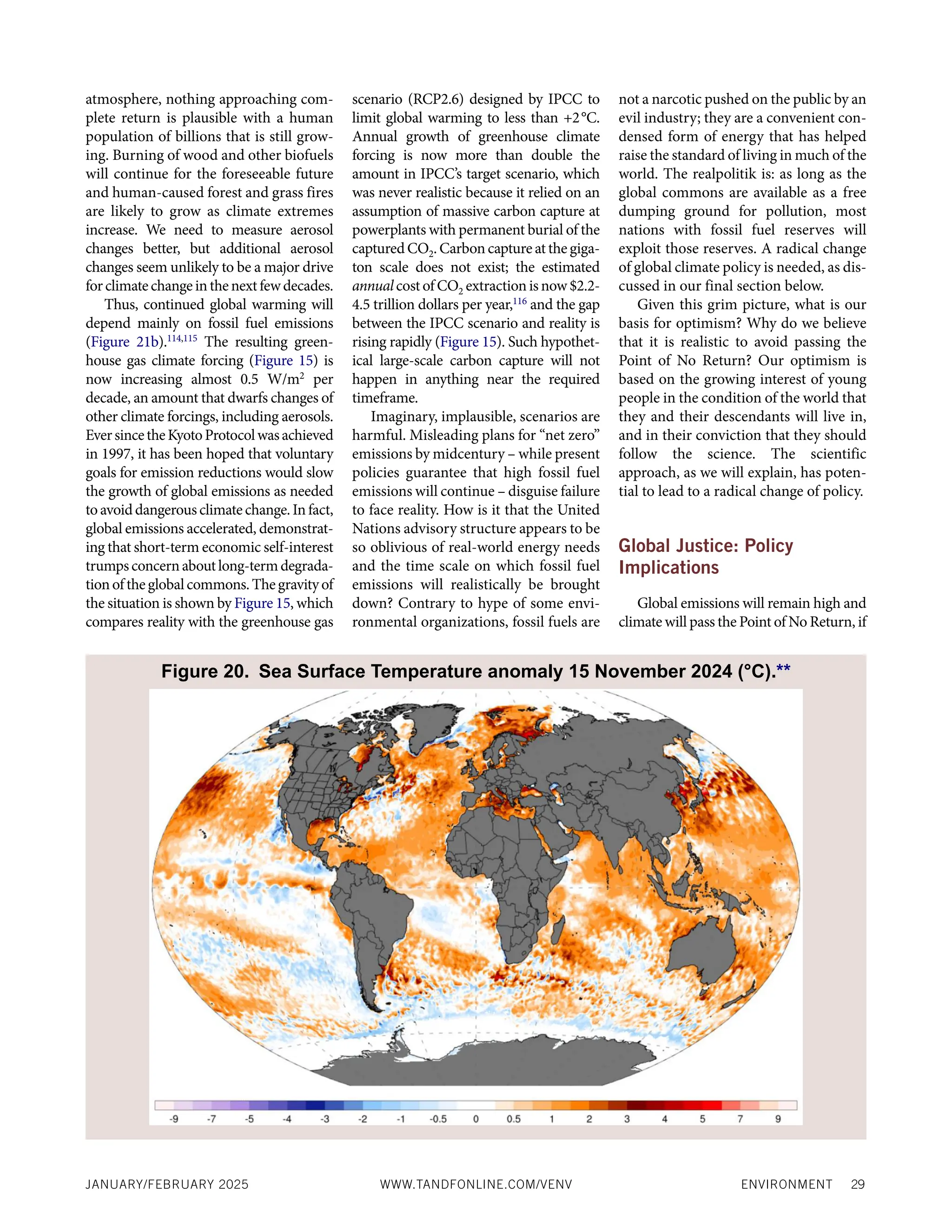
recent SSTs is Figure 20, sea surface temperature
anomalies for 15 November 2024 (from University
of Maine ClimateReanalyzer.org based on NOAA’s
SST anomaly relative to 1971-2000) are typical of
the real world, much cooler in the Southern Ocean
than the models that IPCC relies on.
113. These would show up as unusual change of atmo-
spheric composition or surface properties, which
are not observed.
114. Hefner M, Marland G, Boden T et al. Global,
Regional, and National Fossil-Fuel CO2 Emissions,

40. 44 ENVIRONMENT WWW.TANDFONLINE.COM/VENV VOLUME 67 NUMBER 1
Research Institute for Environment, Energy,
and Economics, Appalachian State University,
Boone, NC, USA. https://energy.appstate.edu/cdi-
ac-appstate/data-products (20 August 2023, date
last accessed).
115. Energy Institute. 2023 Statistical Review of World
Energy (20 August 2023, date last accessed).
116. Assuming empirical cost estimates of 451-924 Tn
US$/tC, based on a pilot direct-air CO2 capture
plant. See J. Hansen, P. Kharecha, “Cost of carbon
capture: Can young people bear the burden?” Joule
2 (2018): 1405-7.
117. J. Hansen, M. Sato, R. Ruedy et al., “Dangerous hu-
man-made interference with climate: A GISS mod-
elE study,” Atmos Chem Phys 7 (2007): 2287-312.
118. H.D. Matthews, N.P. Gillett, P.A. Stott et al., “The
proportionality of global warming to cumulative
carbon emissions,” Nature 459 (2009): 829-32.
119. The economists’ statement on carbon dividends,
3500 economists agree on carbon fee and dividend,
January 2019.
120. Themoneywouldautomaticallybeaddedmonthlyor
quarterly to debit cards of citizens and legal residents.
121. Student leadership on climate solutions, The largest
statement of student government leaders in U.S.
history, 31 July 2020.
122. Can young people save democracy and the planet?
High schoolers for carbon dividends, 8 October
2021.
123. J. Hansen, “Energy for the world,” Draft Chapter 43
in Sophie’s Planet. New York: Bloomsbury, 2025).
124. P.A. Kharecha, J.E. Hansen, “Prevented mortality
and greenhouse gas emissions from historical and
projected nuclear power,” Environ. Sci. Technol., 47
(2013): 4889-95, doi:10.1021/es3051197.
125. A.E. Walter, A.J. Gonzalez, L.E. Feinendegen,
“Why low-level radiation exposure should not be
feared,” Health Phys. 125 no. 3 (2003): September.
126. National Academies of Sciences, Engineering,
and Medicine. 2021. Reflecting Sunlight: Recom­
mendations for Solar Geoengineering Research
and Research Governance. Washington, DC: The
National Academies Press, 328 pp. https://doi.
org/10.17226/25762.
127. P.J. Rasch, S. Tilmes, R.P. Turco et al., “An overview
of geoengineering of climate using stratospheric
sulphate aerosols,” Phil. Trans. Roy. Soc. A 366
(2008): 1882, doi.org/10.1098/rsta.2008.0131.
128. P.J. Crutzen, “Albedo enhancement by stratospher-
ic sulfur injections: A contribution to resolve a pol-
icy dilemma?” Clim. Change 77 (2006): 211– 20,
doi:10.1007/s10584-006-9101-y.
129. J. Hansen, “Aerosol effects on climate and human
health,” https://www.columbia.edu/~jeh1/2018/China_
Charts_Handout_withNotes.pdf, 17 October 2018.
130. A. Jenkins, C. Doake, “Ice-ocean interaction on
Ronne Ice Shelf, Antarctica,” J. Geophys. Res. 96
(1991): 791-813.
131. E. Rignot, S. Jacobs, J. Mouginot et al., “Ice shelf
melting around Antarctica,” Science 341 (2013):
266-70.
132. Figures17and32aintheIceMeltpaper(reference49).
133. K.L. Gunn, S.R. Rintoul, M.H. England et al.,
“Recent reduced abyssal overturning and ventila-
tion in the Australian Antarctic basin,” Nature
Clim. Change 13 (2023): 537-44.
134. L. Cheng, J. Abraham, J. Zhu et al., “Record-setting
warmth continued in 2019,” Adv. Atmos. Sci. 37
(2020): 137-42.
135. J. Sutter, A Jones, T.L. Frolicher et al., “Climate in-
tervention on a high-emissions pathway could de-
lay but not prevent West Antarctic ice sheet de-
mise,” Nature Clim. Chan. 13 (2023): 951-60.
136. P.B. Goddard, B. Kravits, D.G. MacMartin et al.,
“Stratospheric aerosol injection can reduce risks to
Antarctic ice loss depending on injection location
and amount,” J. Geophys. Res.: Atmos. 128 (2023):
e2023JD039434.
137. J.C. Moore, C. Yue, Y. Chen et al., “Multi-model
simulation of solar geoengineering indicates avoid-
able destabilization of the West Antarctic ice sheet,”
Earth’s Future 12 (2024): e2024EF004424.
138. See CO2 graphs at https://www.columbia.edu/~jeh1/
Data/.
139. M. Kilian, S. Brinkop, P. Jockel, “Impact of the
eruption of Mt Pinatubo on the chemical composi-
tion of the stratosphere,” Atmos. Chem. Phys. 20
(2020): 11697-715.
140. K.E. Trenberth, A. Dai, “Effects of Mount Pinatubo
volcanic eruption on the hydrological cycle as an
analog of geoengineering,” Geophys. Res. Lett. 34
(2007): L15702, doi:10.1029/2007GL030524.
141. J. Latham, “Control of global warming?” Nature
347 (1990): 339-40.
142. The already extensive literature on marine cloud
brightening can be found from papers available from
the research program at the University of Washington.
143. C. Merk, G. Pönitzsch, K.Rehdanz, “Knowledge
about aerosol injection does not reduce individual
mitigation efforts,” Global Environ. Change 39
(2016): 302-10.
144. T.L. Cherry, S. Kroll, D.M. McEvoy et al. “2023).
“Climate cooperation in the shadow of solar geoen-
gineering: An experimental investigation of the
moral hazard conjecture,” Environ. Politics 32
(2023): 362–70.
145. P. Schoenegger, K. Mintz-Woo, “Moral hazards and
solar radiation management: Evidence from a
large-scale online experiment,” Jour. Environ.
Psychology 95 (2024): 102288. https://www.sci-
encedirect.com/science/article/pii/S0272494424
000616?via%3Dihub.
146. M. Sugiyama, S. Asayama, T. Kosugi, “The North–
South Divide on Public Perceptions of Stratospheric
Aerosol Geoengineering? A Survey in Six Asia-
Pacific Countries,” Environ. Comm. 14 (2020): 641-56.
147. C.M. Baum, L. Fritz, S. Low et al., “Public percep-
tions and support of climate intervention technolo-
gies across the Global North and Global South,”
Nat Commun 15 (2024): 2060 https://doi.
org/10.1038/s41467-024-46341-5.
148. N. Contzen, G, Perlaviciute, L. Steg et al., “Public
opinion about solar radiation management: A
cross-cultural study in 20 countries around the
world,” Clim. Change 177 (2024): 65 https://doi.
org/10.1007/s10584-024-03708-3.
149. Paris Agreement 2015, UNFCCC secretariat, (last
access 20 August 2023), 2015.
150. Don’t be tricked into using loess-smoothed data,
which make pretty graphs but hide the physics.
151. P. Ditlevsen, S. Ditlevsen, “Warning of a forthcom-
ing collapse of the Atlantic meridional overturning
circulation,” Nature Comm. 14 (2023): doi.
org/10.1038/s41467-023-39810-w.
152. C. Hickman, E. Marks, P. Pihkala et al., “Climate
anxiety in children and young people and their be-
liefs about government responses to climate
change: a global survey,” Lancet Planet Health 5
(2021): e863-73.
153. M.A. Goodman, National Insecurity: The Cost of
American Militarism, City Lights Publishers
(2013): 464 pp.
154. J.F. Kennedy, Peace Speech, American University
Commencement Address, Washington, 10 June
1963.
155. J.K. Galbraith, “Exit Strategy: In 1963, JFK ordered
a complete withdrawal from Vietnam,” Boston
Review, 1 September 2003.
156. S.Wertheim,“HowManyWarsIsAmericaFighting?”
The Gravel Institute, last access 5 January 2023.
157. J.F. Kennedy, “The City Upon a Hill,” speech to
Massachusetts General Assembly, Boston, 9
January 1961.
158. J. Hansen, “Greenhouse Giants,” Draft Chapter 15
in Sophie’s Planet, New York: Bloomsbury, 2025.
159. Already by 1984 the combination of paleoclimate
data and global climate modeling was shown to
imply a climate sensitivity 2.5-5°C for doubled
CO2 [J. Hansen, A. Lacis, D. Rind et al., “Climate
sensitivity: analysis of feedback mechanisms,” In:
J.E. Hansen, T. Takahashi (eds). AGU Geophysical
Monograph 29 Climate Processes and Climate
Sensitivity. Washington: American Geophysical
Union (1984): 130-63] with the large range main-
ly caused by uncertainty in the magnitude of gla-
cial/interglacial temperature change. A recent re-
markable analysis of noble gas abundances in
groundwater deposited during the last ice age [A.
M. Seltzer, J. Ng, W. Aeschbach et al., “Widespread
six degrees Celsius cooling on land during the
Last Glacial Maximum,” Nature 593 (2021): 228-
32] favors climate sensitivity in the range 4-5°C
for doubled CO2 (see discussion the Seltzer paper
in reference 1).
160. Kyoto Protocol, 1997: http://unfccc.int/kyoto_pro-
tocol/items/2830.php (last access: 20 November
2024).
161. J. Hansen, “Carbon Tax and 100% Dividend” com-
munication and presentation, 3 and 4 June 2008;
also in a letter to President-elect Obama in
December 2008.
162. P. Barnes, “Cap and dividend testimony before
House Ways and Means Committee,” 18 September
2008.
163. Editors of Encyclopedia Britannica, Kyoto
Protocol, last updated 11 November 2024.
164. J. Hansen, M. Sato, R. Ruedy et al., “Global warm-
ing in the twenty-first century: an alternative sce-
nario,” Proc Natl Acad Sci 97 (2000): 9875-80.
165. Gerry Lenfest, who explained his munificence to
an Iowa native, by noting that, as an idle teen-ager,
he was sent by his father to work on an Iowa farm,
where, he decided, Iowans “were honest and
worked hard.” U.S. science agencies also contribut-
ed support for the first (2002) workshop.
166. J. Hansen (ed.), “Air Pollution as a Climate
Forcing,” report of a workshop in Honolulu, 29
April-3 May 2002.
167. The symposium, with foresight, covered two top-
ics: climate and human health. The other invited
scientist from the U.S., Tom Frieden, Director of
the Centers for Disease Control, was invited to
lead on public health and infectious disease.
Frieden did not attend, but was represented by his
deputy.
168. J. Hansen, “Beijing Charts: shown at Symposium
on a New Type of Major Power Relationship:
Counsellors Office of the State Council of the
People’s Republic of China and the Kissinger
Institute on China and the United States.
169. J. Hansen, “Sleepless in Ningbo: a note concerning a
visit to China and a draft op-ed on climate injustice.
170. J. Hansen, “World’s Greatest Crime against
Humanity and Nature,” was written as an op-ed
and submitted to a Chinese newspaper while I was
in China. It was never published there, but on the
editor’s invitation, a revised version was published
in Chemistry World as The Energy to Fight
Injustice.
171. J. Cao, A. Cohen, J. Hansen et al., “China-U.S. co-
operation to advance nuclear power,” Science 353
(2016): 547-8.
172. Armenia, Bulgaria, Canada, Croatia, Czech
Republic, El Salvador, Finland, France, Ghana,
Hungary, Jamaica, Japan, Kazakhstan, Kenya,
Republic of Korea, Kosovo, Moldova, Mongolia,
Morocco, Netherlands, Nigeria, Poland, Romania,
Slovakia, Slovenia, Sweden, Turkey, Ukraine,
United Arab Emirates, United Kingdom, United
States.
173. J. Hansen, “Sack Goldman Sachs Cap-and-Trade” 7
December 2009 communication on Columbia
website.
174. A trenchant response by MarkB at 11:05 AM on 7
December2009: “…The entire cap and trade legis-
lation is written to extract rents for special inter-
ests. And it actually GUARANTEES coal fired
power into the future. Krugman is like Colonel
Nicholson in the movie Bridge on the River Kwai,
the British officer in a Japanese POW prison who
drives his men to build a bridge to keep morale up
– forgetting that the bridge is meant to aid the
Japanese war effort. Krugman is so dedicated to
“the cause” that he can’t see – like Jim Hansen
does – that cap and trade will actually harm the
cause in the end. The big energy companies are
lined up IN FAVOR of cap and trade – think
about it.”
175. The Economists’ Statement on Carbon Dividends,
Website of Students for Carbon Dividends.