Exp19_Excel_App_Cap_Comp_Tech_Store_Instructions.docx
Grader - Instructions Excel 2019
ProjectExp19_Excel_App_Cap_Comp_Tech_Store
Project Description:
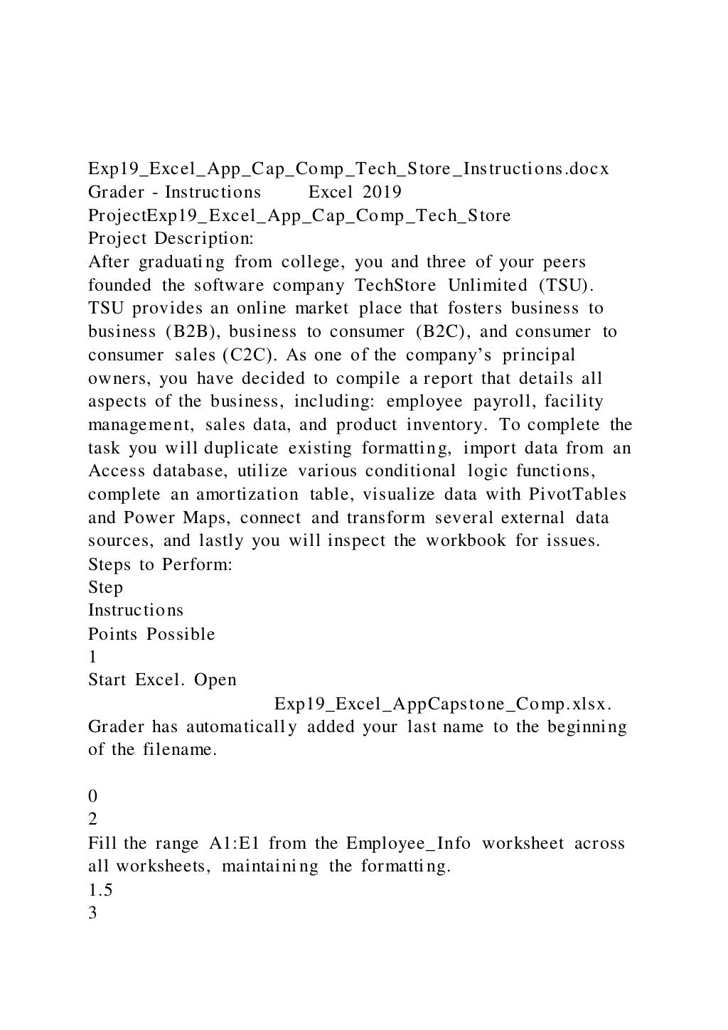
After graduating from college, you and three of your peers
founded the software company TechStore Unlimited (TSU).
TSU provides an online market place that fosters business to
business (B2B), business to consumer (B2C), and consumer to
consumer sales (C2C). As one of the company’s principal
owners, you have decided to compile a report that details all
aspects of the business, including: employee payroll, facility
management, sales data, and product inventory. To complete the
task you will duplicate existing formatting, import data from an
Access database, utilize various conditional logic functions,
complete an amortization table, visualize data with PivotTables
and Power Maps, connect and transform several external data
sources, and lastly you will inspect the workbook for issues.
Steps to Perform:
Step
Instructions
Points Possible
1
Start Excel. Open
Exp19_Excel_AppCapstone_Comp.xlsx.
Grader has automatically added your last name to the beginning
of the filename.
0
2
Fill the range A1:E1 from the Employee_Info worksheet across
all worksheets, maintaining the formatting.
1.5
3
Make the New_Construction worksheet active and create Range
Names based on the data in the range A6:B9.
1.5
4
Ungroup the worksheets and ensure the Employee_Info
worksheet is active. Click cell G6 and enter a nested logical
function that calculates employee 401K eligibility. If the
employee is full time (FT) and was hired before the 401k cutoff
date 1/1/19, then he or she is eligible and
Y should be displayed, non-eligible
employees should be indicated with a
N. Be sure to utilize the date located in
cell H3 as a reference in the formula. Use the fill handle to copy
the function down completing the range G6:G25.
2.5
5
Apply conditional formatting to the range G6:G25 that
highlights eligible employees with Green Fill with Dark Green
text. Eligible employees are denoted with a Y in column G.
1.5
6
Create a Data Validation list in cell J7 based on the employee
IDs located in the range A6:A25. Add the Input Message
Select Employee ID and use the Stop Style
Error Alert.
1.5
7
Enter a nested INDEX and MATCH function in cell K7 that
examines the range B6:H25 and returns the corresponding
employee information based on the match values in cell J7 and
cell K6. Note K6 contains a validation list that can be used to
select various lookup categories. Use the Data Validation list in
cell J7 to select Employee_ID
31461 and select
Salary in cell K6 to test the function.
2
8
Enter a conditional statistical function in cell K14 that
calculates the total number of
PT employees. Use the range E6:E25 to
complete the function.
1.5
9
Enter a conditional statistical function in cell K15 that
calculates the total value of
PT employee salaries. Use the range
E6:E25 to complete the function.
1.5
10
Enter a conditional statistical function in cell K16 that
calculates the average value of
PT employee salaries. Use the range
E6:E25 to complete the function.
1.5
11
Enter a conditional statistical function in cell K17 that
calculates the highest
PT employee salary. Use the range E6:E25
to complete the function.
1.5
12
Apply Currency Number Format to the range K15:K17.
0.5
13
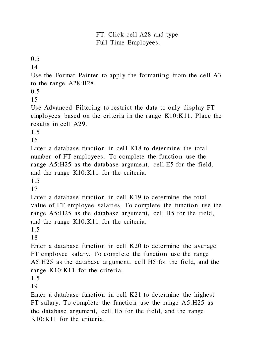
Click cell K11 and type
FT. Click cell A28 and type
Full Time Employees.
0.5
14
Use the Format Painter to apply the formatting from the cell A3
to the range A28:B28.
0.5
15
Use Advanced Filtering to restrict the data to only display FT
employees based on the criteria in the range K10:K11. Place the
results in cell A29.
1.5
16
Enter a database function in cell K18 to determine the total
number of FT employees. To complete the function use the
range A5:H25 as the database argument, cell E5 for the field,
and the range K10:K11 for the criteria.
1.5
17
Enter a database function in cell K19 to determine the total
value of FT employee salaries. To complete the function use the
range A5:H25 as the database argument, cell H5 for the field,
and the range K10:K11 for the criteria.
1.5
18
Enter a database function in cell K20 to determine the average
FT employee salary. To complete the function use the range
A5:H25 as the database argument, cell H5 for the field, and the
range K10:K11 for the criteria.
1.5
19
Enter a database function in cell K21 to determine the highest
FT salary. To complete the function use the range A5:H25 as
the database argument, cell H5 for the field, and the range
K10:K11 for the criteria.
1.5
20
Format the range K19:K21 with Currency Number Format.
0.5
21
Ensure that the New_Construction worksheet is active. Use
Goal Seek to reduce the monthly payment in cell B6 to the
optimal value of $8000. Complete this task by changing the
Loan amount in cell E6.
2.5
22
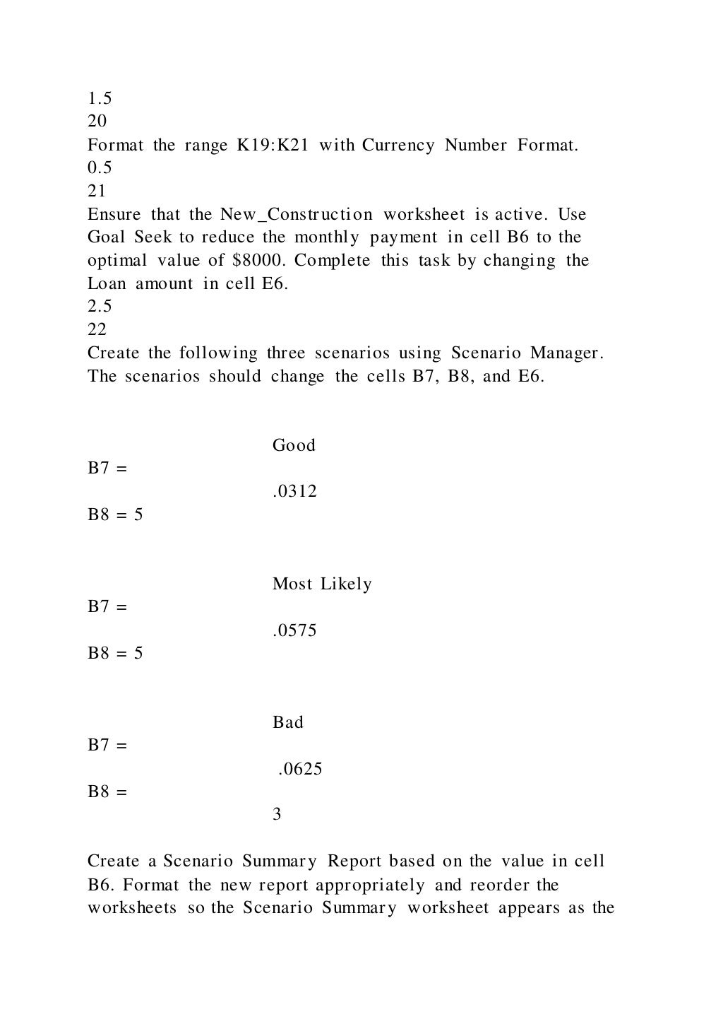
Create the following three scenarios using Scenario Manager.
The scenarios should change the cells B7, B8, and E6.
Good
B7 =
.0312
B8 = 5
Most Likely
B7 =
.0575
B8 = 5
Bad
B7 =
.0625
B8 =
3
Create a Scenario Summary Report based on the value in cell
B6. Format the new report appropriately and reorder the
worksheets so the Scenario Summary worksheet appears as the
last worksheet in the workbook.
4.5
23
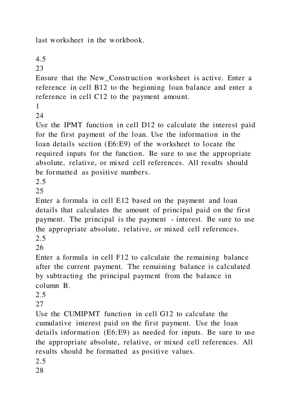
Ensure that the New_Construction worksheet is active. Enter a
reference in cell B12 to the beginning loan balance and enter a
reference in cell C12 to the payment amount.
1
24
Use the IPMT function in cell D12 to calculate the interest paid
for the first payment of the loan. Use the information in the
loan details section (E6:E9) of the worksheet to locate the
required inputs for the function. Be sure to use the appropriate
absolute, relative, or mixed cell references. All results should
be formatted as positive numbers.
2.5
25
Enter a formula in cell E12 based on the payment and loan
details that calculates the amount of principal paid on the first
payment. The principal is the payment - interest. Be sure to use
the appropriate absolute, relative, or mixed cell references.
2.5
26
Enter a formula in cell F12 to calculate the remaining balance
after the current payment. The remaining balance is calculated
by subtracting the principal payment from the balance in
column B.
2.5
27
Use the CUMIPMT function in cell G12 to calculate the
cumulative interest paid on the first payment. Use the loan
details information (E6:E9) as needed for inputs. Be sure to use
the appropriate absolute, relative, or mixed cell references. All
results should be formatted as positive values.
2.5
28
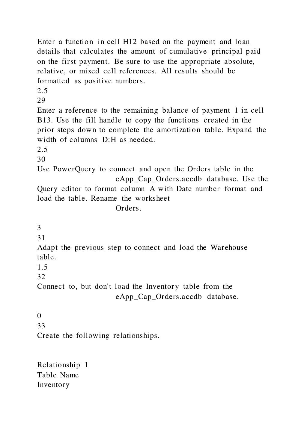
Enter a function in cell H12 based on the payment and loan
details that calculates the amount of cumulative principal paid
on the first payment. Be sure to use the appropriate absolute,
relative, or mixed cell references. All results should be
formatted as positive numbers.
2.5
29
Enter a reference to the remaining balance of payment 1 in cell
B13. Use the fill handle to copy the functions created in the
prior steps down to complete the amortization table. Expand the
width of columns D:H as needed.
2.5
30
Use PowerQuery to connect and open the Orders table in the
eApp_Cap_Orders.accdb database. Use the
Query editor to format column A with Date number format and
load the table. Rename the worksheet
Orders.
3
31
Adapt the previous step to connect and load the Warehouse
table.
1.5
32
Connect to, but don't load the Inventory table from the
eApp_Cap_Orders.accdb database.
0
33
Create the following relationships.
Relationship 1
Table Name
Inventory
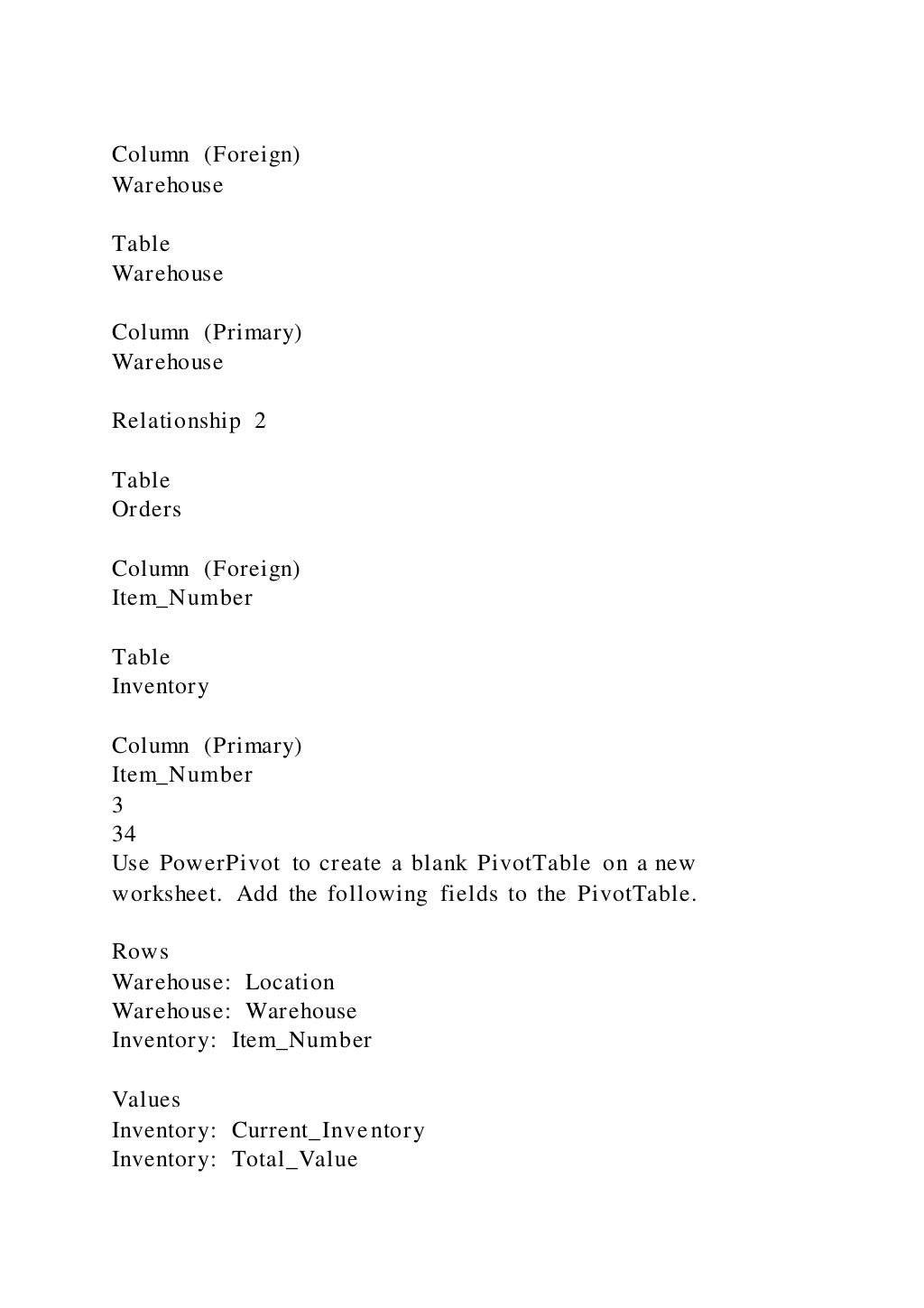
Column (Foreign)
Warehouse
Table
Warehouse
Column (Primary)
Warehouse
Relationship 2
Table
Orders
Column (Foreign)
Item_Number
Table
Inventory
Column (Primary)
Item_Number
3
34
Use PowerPivot to create a blank PivotTable on a new
worksheet. Add the following fields to the PivotTable.
Rows
Warehouse: Location
Warehouse: Warehouse
Inventory: Item_Number
Values
Inventory: Current_Inventory
Inventory: Total_Value
4
35
Insert a Slicer based on Warehouse. Place the upper left corner
of the Slicer inside the borders of cell F3.
1.5
36
Create a 3D PowerMap that displays the location of all
warehouses based on the City geographic type. Rename the
worksheet
Inventory.
1
37
Make the Orders worksheet active. Use the Data Analysis
ToolPak to output Summary statistics starting in cell G3. The
statistics should be based on the quantity of orders located in
the range E1:E50. Be sure to include column headings in the
output.
1.5
38
Record a macro using the Macro Recorder named
Sort. When activated, the macro should
sort the Orders table in ascending order by date. Open the newly
created module in the Visual Basic Editor and copy the code in
Module1. Paste the code starting in cell A1 on the Code
worksheet.
2.5
39
On the Orders worksheet, insert a Form Control button labeled
Sort in the range G21:I24 and assign the
Sort macro.
2
40
Use the Accessibility Checker to inspect for issues. Once
located, make the following changes to alleviate the issues.
Warehouse worksheet
Change Table Style to none.
Orders worksheet
Change Table Style to none.
Employee_Info worksheet
Change Font Color to Black, Text 1
New_Construction worksheet
Change Font Color to Black, Text 1
Save the file
Exp19_Excel_AppCapstone_Comp.xlsx.
Exit Excel. Submit the file as directed.
1
Total Points
70
Created On: 05/05/2022 1 Exp19_Excel_App_Cap_Comp -
Tech Store 1.6
Whiting_Exp19_Excel_AppCapstone_Comp.xlsx
Employee_InfoTech Store UnlimitedEmployee Information401K
Cut
Off1/1/19Employee_IDStart_DateFirst_NameLast_NameTypeDe
pendents401k EligibleSalaryEmployee
Lookup314612/1/17NelsonGailFT1$
125,000.00Employee_IDDependents567688/19/20LopezVivianF
T4$ 100,000.00314281/8/17RamseyMatthewFT0$
110,000.00462742/2/17StevensonBeverlyFT3$
85,000.00Employee LookupFilter302614/29/20SmithPeterFT0$
95,000.00Employee_IDTypeDependentsSalary434821/21/19Kell
eyEmilyPT2$ 18,864.00886965/1/21CarrollPhyllisPT3$
23,722.00650301/28/18HuntBarbaraPT0$ 14,966.00Employee
Statistics9867412/29/18AustinMelaniePT4$ 18,751.00#
PT9806510/14/20SnyderJeanPT1$ 18,875.00Total PT
Salaries800876/4/20MorrisSuzannePT3$ 11,513.00Average PT
Salary798866/15/18GibsonGeraldinePT0$ 20,044.00Highest
PT Salary6440111/3/21GrahamVickiPT3$ 10,354.00#
FT7292212/15/21WatsonMarilynPT4$ 11,049.00Total FT
Salaries908715/30/19SimpsonTroyPT3$ 24,010.00Average FT
Salary399481/14/20BarberAaronPT4$ 11,156.00Highest FT
Salary4072512/7/20MoralesBrittanyPT3$
23,142.00429881/31/19BlairCynthiaPT3$
12,105.00404994/13/18JenningsDoloresPT0$
24,905.00282534/29/18CarrollHowardPT3$ 10,663.00
New_ConstructionFacility Amortization TablePayment
DetailsLoan
DetailsPayment$8,647.55Loan$450,000.00APR5.75%Periodic
Rate0.479%Years5# of Payments60Pmts per Year12Payment
NumberBeginning BalancePayment AmountInterest
PaidPrincipal RepaymentRemaining BalanceCumulative
InterestCumulative
Principal123456789101112131415161718192021222324252627
28293031323334353637383940414243444546474849505152535
4555657585960Totals$ - 0$ - 0
Code
Exp19_Excel_App_Cap_Comp_Tech_Store_final_result.jpg
eApp_Cap_Orders.accdbItem_NumberUnit_CostWarehouseCurr
ent_InventoryTotal_Value1112.0¤ 819.00C274.0¤ 224,406.0012
32.0¤ 318.00A149.0¤ 47,382.001265.0¤ 461.00C146.0¤ 67,306.
001304.0¤ 381.00A145.0¤ 55,245.001329.0¤ 903.00C44.0¤ 39,7
32.001464.0¤ 564.00C47.0¤ 26,508.001611.0¤ 688.00A60.0¤ 41
,280.001648.0¤ 502.00C270.0¤ 135,540.002007.0¤ 502.00C251.
0¤ 126,002.002079.0¤ 812.00C227.0¤ 184,324.002130.0¤ 263.0
0A36.0¤ 9,468.002496.0¤ 680.00C153.0¤ 104,040.002583.0¤ 45
4.00B96.0¤ 43,584.003411.0¤ 186.00A2.0¤ 372.003464.0¤ 402.
00D225.0¤ 90,450.003706.0¤ 766.00D63.0¤ 48,258.003939.0¤ 7
44.00A27.0¤ 20,088.004697.0¤ 861.00B143.0¤ 123,123.005089.
0¤ 249.00E300.0¤ 74,700.005160.0¤ 592.00B135.0¤ 79,920.005
421.0¤ 930.00A157.0¤ 146,010.005824.0¤ 852.00B98.0¤ 83,496
.005906.0¤ 872.00B262.0¤ 228,464.006076.0¤ 198.00A75.0¤ 14
,850.006257.0¤ 526.00A253.0¤ 133,078.006263.0¤ 792.00B66.0
¤ 52,272.006466.0¤ 594.00C36.0¤ 21,384.006685.0¤ 351.00B26
7.0¤ 93,717.006871.0¤ 742.00B231.0¤ 171,402.006884.0¤ 197.
00B126.0¤ 24,822.007082.0¤ 379.00A96.0¤ 36,384.007333.0¤ 1
93.00A43.0¤ 8,299.007361.0¤ 481.00A241.0¤ 115,921.007508.0
¤ 488.00A10.0¤ 4,880.007553.0¤ 622.00A31.0¤ 19,282.007636.
0¤ 57.00B15.0¤ 855.007640.0¤ 277.00A23.0¤ 6,371.007664.0¤
847.00C2.0¤ 1,694.008107.0¤ 666.00D139.0¤ 92,574.008342.0¤
16.00A197.0¤ 3,152.008368.0¤ 320.00B189.0¤ 60,480.008547.
0¤ 590.00A111.0¤ 65,490.008611.0¤ 591.00D36.0¤ 21,276.0093
79.0¤ 28.00A217.0¤ 6,076.009398.0¤ 148.00C204.0¤ 30,192.00
9423.0¤ 393.00C104.0¤ 40,872.009443.0¤ 982.00A185.0¤ 181,6
70.009482.0¤ 661.00E252.0¤ 166,572.009744.0¤ 716.00E65.0¤
46,540.009824.0¤ 769.00B47.0¤ 36,143.00DateOrder_IDItem_N
umberSupplier_NumberQuantity2020-01-
011000.06884.05446.011.02020-01-
081001.09482.05446.016.02020-01-
141002.03939.04165.09.02020-01-
251003.07333.03437.021.02020-01-
271004.02583.05446.03.02020-02-
071005.06871.03437.011.02020-02-
221006.09423.07741.011.02020-03-
041007.05421.05446.023.02020-03-
071008.07333.05446.016.02020-03-
121009.09398.05446.08.02020-03-
231010.08107.03437.022.02020-03-
261011.07082.04165.021.02020-04-
031012.08342.03437.022.02020-04-
041013.07333.05446.03.02020-04-
091014.01329.07741.019.02020-04-
131015.09482.03437.013.02020-04-
281016.09824.03437.09.02020-05-
031017.07361.03437.022.02020-05-
041018.09423.07741.019.02020-05-
071019.07640.03437.023.02020-05-
291020.06466.07741.011.02020-06-
011021.02130.05446.022.02020-06-
031022.02583.07741.017.02020-07-
061023.06871.07741.021.02020-07-
281024.01304.03437.08.02020-08-
161025.07553.03437.02.02020-08-
191026.07664.05446.011.02020-08-
261027.09423.05446.023.02020-09-
041028.06685.03437.015.02020-09-
091029.02007.05446.016.02020-09-
131030.01304.04165.017.02020-09-
191031.06263.03437.022.02020-09-
201032.02496.03437.012.02020-09-
301033.09379.05446.08.02020-10-
121034.07333.07741.012.02020-10-
141035.05824.07741.023.02020-10-
171036.06257.03437.017.02020-10-
241037.09482.05446.09.02020-10-
301038.09398.07741.03.02020-11-
021039.05824.04165.016.02020-11-
141040.09443.03437.015.02020-11-
251041.07640.05446.01.02020-12-
021042.05421.05446.06.02020-12-
161043.03464.03437.015.02020-12-
191044.06257.05446.019.02020-12-
221045.05089.04165.02.02020-12-
291046.09824.03437.022.02020-12-
301047.05824.07741.023.02020-12-
311048.03706.04165.08.0WarehouseLocationAChicago,
IllinoisBIndianapolis, IndianaCCleveland, OhioDDenver,
ColoradoEPortland, Oregon
Whiting_Exp19_Excel_Ch11_Cap_Donors.xlsx
DonorsLook Up AreaFormulasSummaryDonor ID:ART-39Cell
B3Total Donations:Donor Position:Cell B4Average
donation:Donor Name:Cell D8Total donors:Donor Amount:Cell
K2CollegeCollege IDDonor IDNew Donor IDFull NameLast
NameAddressCityStateCollege/SchoolDonationENGINEERING
15Schneider, Dedrick1243 W Abbey
Rd,Columbus,OH5,000BUSINESS25Beauclair, Oliver34 E
Affinity Dr,Cincinnati,OH7,500BUSINESS27Flores, Adrian912
E Julien Circle,Akron,OH10,000ART45Wang, Shan2945 N
Country Club Rd,Chicago
Heights,IL3,500ENGINEERING22Schafer, Elysia259 S
Wadsbury Dr,Cincinnati,OH4,000ART39Romero, Samantha123
W Lincoln Ave,Dayton,OH6,000ART12Mikhailov, Jon342 S
Newton Dr,Columbus,OH750BUSINESS14Jaundreau, Hunter64
E 111th Place,Chicago,IL500ENGINEERING18Kato, Eiji41 W
Eaton Drive,Toledo,OH1,250ENGINEERING23Schroder,
Genevie6124 N Odelle Dr,Akron,OH3,000ART24Diaz,
Sergio142 S Elm Street,Erie,PA1,255BUSINESS31Lamoureux,
Lucas3415 N Saddlewood Dr,Toledo,OH3,000ART36Acosta,
Jaime1490 S Alcove Way,Pittsburgh,PA855ART42Ishikawa,
Chie4152 E Dalbren
Ln,Cincinnati,OH6,500BUSINESS44Kruger, Alfonso641 W
Banbury Dr,Toledo,OH2,500ART38Normandeau, Amelia45 E
Blackstone Court,Detroit,MI5,555ENGINEERING52Cabrera,
Mia923 W Haldy
Rd,Columbus,OH3,545BUSINESS53Fernandez, Isabella641 S
Caiser Court,San Francisco,CA4,210BUSINESS49Wright,
Jerri64 W Garden Court,Bowling
Green,OH900ENGINEERING47Friedrich, Ava15 E Oak Hill
Drive,Anaheim,CA950ENGINEERING26Byram, Emma324 E
Deer Valley Drive,Park City,UT11,000ART46Renault,
Linden3434 E Wallhaven
Circle,Akron,OH12,500BUSINESS55Sanchez, Caleb25 W
Catherine Street,Ann Arbor,MI2,355ART41Zhang, Jun3914
McCartney Rd,Youngstown,OH900ENGINEERING33Deneau,
Abigail345 N Cobb Place,Detroit,MI1,600BUSINESS58Walker,
Mitchell1850 N Lelanford Cir,Bowling
Green,OH655ART34Perez, Tina45 E Keyes
Ave,Cleveland,OH6,545ENGINEERING58Morgan, Terry1200
E. Monticello Blvd,Cleveland,OH750
Exp19_Excel_Ch11_Cap_Donors_Instructions.docx
Grader - Instructions Excel 2019
ProjectExp19_Excel_Ch11_Cap_Donors
Project Description:
You are a development officer for a state university. As an
officer, you manage a portfolio of important donors who
contribute financially to different areas within the university.
You categorize the donors based on the college or school for
which they want their donations associated. You recently
downloaded the portfolio to an Excel workbook. Based on the
way the data downloads from the main database, you want to
format the text for readability and to make it easier for you to
analyze. In addition, you will create an advanced filter to
review a list of donors for a particular college or school.
Finally, you want to create a look up area to look up data for a
specific donor and create a summary section.
Steps to Perform:
Step
Instructions
Points Possible
1
Start Excel. Download and open the file named
Exp19_Excel_Ch11_Cap_Donors.xlsx.
Grader has automatically added your last name to the beginning
of the filename.
0
2
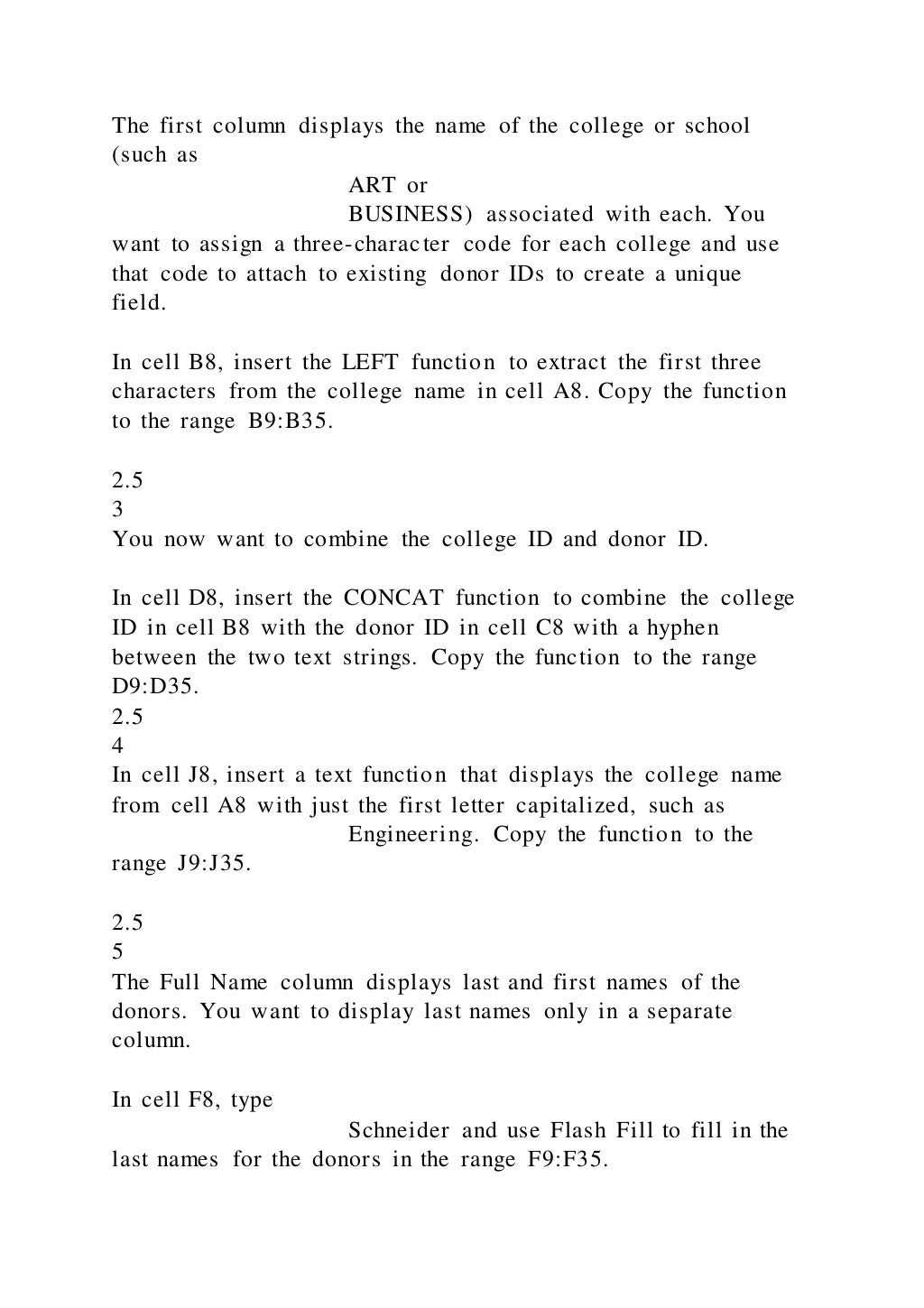
The first column displays the name of the college or school
(such as
ART or
BUSINESS) associated with each. You
want to assign a three-character code for each college and use
that code to attach to existing donor IDs to create a unique
field.
In cell B8, insert the LEFT function to extract the first three
characters from the college name in cell A8. Copy the function
to the range B9:B35.
2.5
3
You now want to combine the college ID and donor ID.
In cell D8, insert the CONCAT function to combine the college
ID in cell B8 with the donor ID in cell C8 with a hyphen
between the two text strings. Copy the function to the range
D9:D35.
2.5
4
In cell J8, insert a text function that displays the college name
from cell A8 with just the first letter capitalized, such as
Engineering. Copy the function to the
range J9:J35.
2.5
5
The Full Name column displays last and first names of the
donors. You want to display last names only in a separate
column.
In cell F8, type
Schneider and use Flash Fill to fill in the
last names for the donors in the range F9:F35.
2.5
6
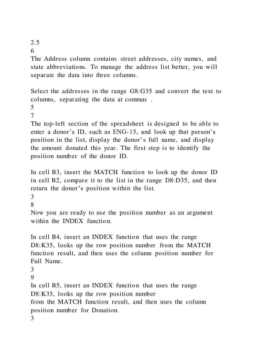
The Address column contains street addresses, city names, and
state abbreviations. To manage the address list better, you will
separate the data into three columns.
Select the addresses in the range G8:G35 and convert the text to
columns, separating the data at commas .
5
7
The top-left section of the spreadsheet is designed to be able to
enter a donor’s ID, such as ENG-15, and look up that person’s
position in the list, display the donor’s full name, and display
the amount donated this year. The first step is to identify the
position number of the donor ID.
In cell B3, insert the MATCH function to look up the donor ID
in cell B2, compare it to the list in the range D8:D35, and then
return the donor’s position within the list.
3
8
Now you are ready to use the position number as an argument
within the INDEX function.
In cell B4, insert an INDEX function that uses the range
D8:K35, looks up the row position number from the MATCH
function result, and then uses the column position number for
Full Name.
3
9
In cell B5, insert an INDEX function that uses the range
D8:K35, looks up the row position number
from the MATCH function result, and then uses the column
position number for Donation.
3
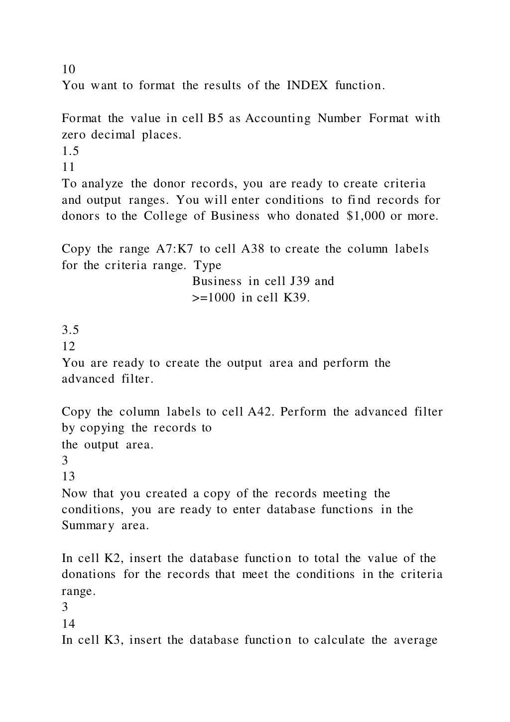
10
You want to format the results of the INDEX function.
Format the value in cell B5 as Accounting Number Format with
zero decimal places.
1.5
11
To analyze the donor records, you are ready to create criteria
and output ranges. You will enter conditions to find records for
donors to the College of Business who donated $1,000 or more.
Copy the range A7:K7 to cell A38 to create the column labels
for the criteria range. Type
Business in cell J39 and
>=1000 in cell K39.
3.5
12
You are ready to create the output area and perform the
advanced filter.
Copy the column labels to cell A42. Perform the advanced filter
by copying the records to
the output area.
3
13
Now that you created a copy of the records meeting the
conditions, you are ready to enter database functions in the
Summary area.
In cell K2, insert the database function to total the value of the
donations for the records that meet the conditions in the criteria
range.
3
14
In cell K3, insert the database function to calculate the average
donation for the records that meet the conditions in the criteria
range.
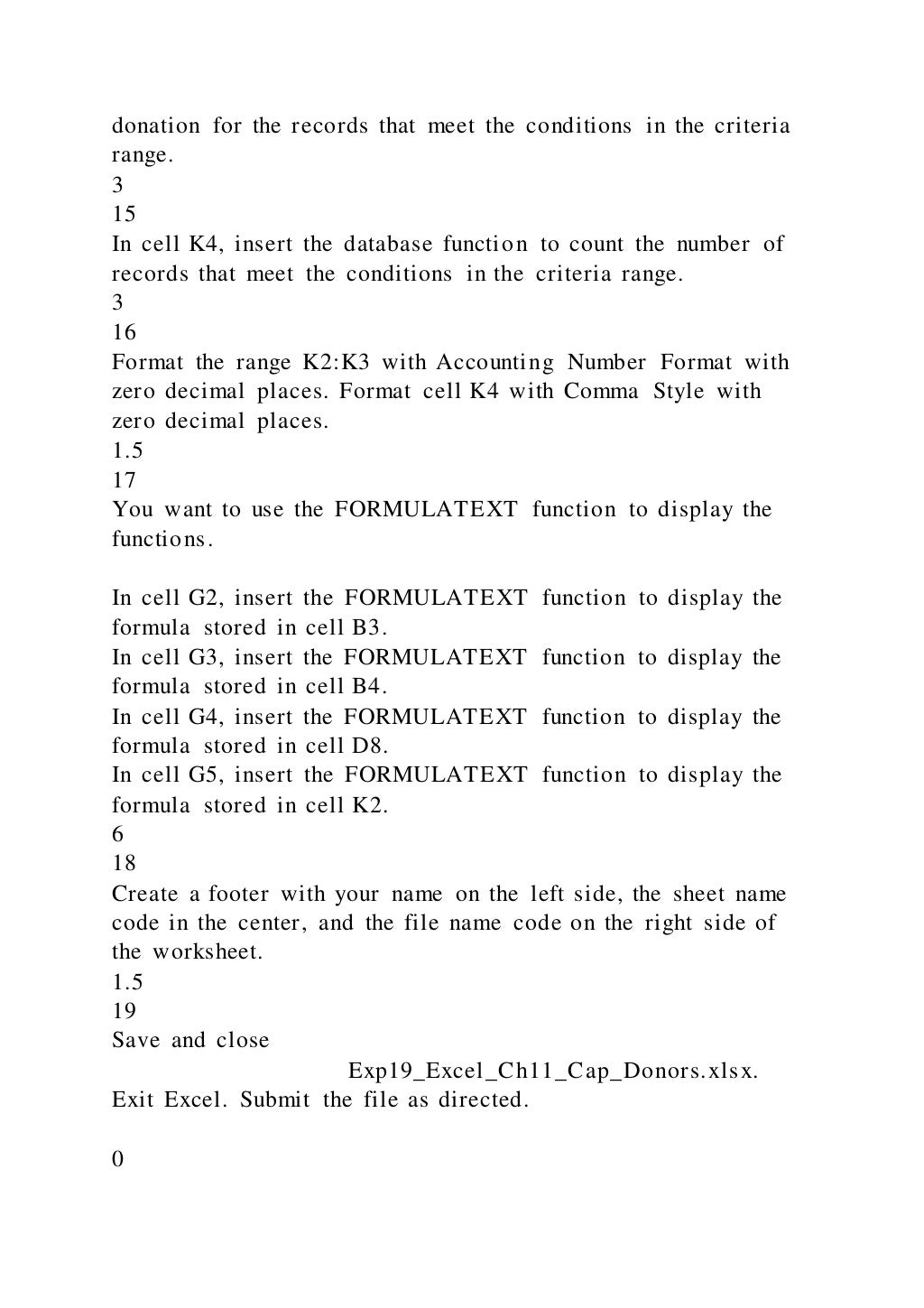
3
15
In cell K4, insert the database function to count the number of
records that meet the conditions in the criteria range.
3
16
Format the range K2:K3 with Accounting Number Format with
zero decimal places. Format cell K4 with Comma Style with
zero decimal places.
1.5
17
You want to use the FORMULATEXT function to display the
functions.
In cell G2, insert the FORMULATEXT function to display the
formula stored in cell B3.
In cell G3, insert the FORMULATEXT function to display the
formula stored in cell B4.
In cell G4, insert the FORMULATEXT function to display the
formula stored in cell D8.
In cell G5, insert the FORMULATEXT function to display the
formula stored in cell K2.
6
18
Create a footer with your name on the left side, the sheet name
code in the center, and the file name code on the right side of
the worksheet.
1.5
19
Save and close
Exp19_Excel_Ch11_Cap_Donors.xlsx.
Exit Excel. Submit the file as directed.
0
Total Points
50
Created On: 06/12/2020 1 Exp19_Excel_Ch11_Cap -
Donors 1.0
Exp19_Excel_Ch11_Cap_Donors_final_result.jpg
Whiting_EXP19_Excel_Ch12_Cap_Inventory.xlsx
Inventory ListINVENTORY LISTTOTAL INVENTORY
VALUE:INVENTORY ITEMS:BIN COUNT:INVENTORY
PICK LISTBIN LOOKUP$4,649.00116SKUDESCRIPTIONBIN
#LOCATIONUNITQTYREORDER QTYCOSTINVENTORY
VALUEREORDERSP7875Item 1T345Row 2, slot
1Each2010$30.00$600.00TR87680Item 2T345Row 2, slot
1Each3015$40.00$1,200.00MK676554Item 3T5789Row 1, slot
1Each105$5.00$50.00YE98767Item 4T9876Row 3, slot 2Box
(10 ct)4010$15.00$600.00XR23423Item 5T098Row 3, slot
1Each1210$26.00$312.00PW98762Item 6T345Row 2, slot
1Each710$50.00$350.00ReorderBM87684Item 7T349Row 1,
slot 2Each105$10.00$100.00BH67655Item 8T5789Row 1, slot
1Each1910$3.00$57.00WT98768Item 9T9875Row 2, slot
2Package (5 ct)2030$14.00$280.00ReorderTS3456Item
10T349Row 1, slot 2Each158$60.00$900.00WDG123Ite m
11T349Row 1, slot 2Each2515$8.00$200.00
INVENTORY PICK
LIST/xl/drawings/drawing1.xml#'Inventory%20Pick%20List'!A
1
BIN LOOKUP/xl/drawings/drawing1.xml#'Bin%20Lookup'!A1
Inventory Pick ListINVENTORY PICK LISTINVENTORY
LISTORDER #SKUPICK QTYQTY AVAILABLEITEM
DESCRIPTIONUNITBIN #LOCATIONTP001-1SP7875320Item
1EachT345Row 2, slot 1TP001-1YE98767140Item 4Box (10
ct)T9876Row 3, slot 2TP001-1BM87684210Item
7EachT349Row 1, slot 2TP001-1TS3456615Item
10EachT349Row 1, slot 2TP001-1MK676554310Item
3EachT5789Row 1, slot 1
INVENTORY
LIST/xl/drawings/drawing2.xml#'Warehouse%20Inventory%20L
ist'!A1
CLEAR PICK LIST
Bin LookupBIN LOOKUPINVENTORY LISTBIN
#DESCRIPTIONLOCATIONWIDTHHEIGHTLENGTHT345Lar
ge binRow 2, slot 1501010T5789Small binRow 1, slot
12555T9876Large binRow 3, slot 2501010T098Medium binRow
3, slot 130710T349Small binRow 1, slot 22555T5789Large
binRow 4, slot 5501010T9875Large binRow 2, slot 2501010
INVENTORY
LIST/xl/drawings/drawing3.xml#'Warehouse%20Inventory%20L
ist'!A1
Exp19_Excel_Ch12_Cap_Bulldog_Collectibles_Instructions.doc
x
Grader - Instructions Excel 2019
ProjectExp19_Excel_Ch12_Cap_Bulldog_Collectibles
Project Description:
You are the operations manager for Bulldog collectables, a
small start-up company that deals with sports memorabilia. As
you prepare to document your inventory, you decide to utilize a
template to save time. To complete this task, you will create a
worksheet based on an Office.com template; you will also use
the Macro Recorder and Visual Basic for Application to
automate sorting and calculations within the workbook.
Steps to Perform:
Step
Instructions
Points Possible
1
Start Excel. Download and open the file named
EXP19_Excel_Ch12_Cap_Inventory.xlsx.
Grader has automatically added your last name to the beginning
of the filename.
0
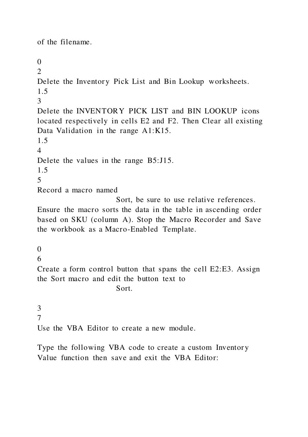
2
Delete the Inventory Pick List and Bin Lookup worksheets.
1.5
3
Delete the INVENTORY PICK LIST and BIN LOOKUP icons
located respectively in cells E2 and F2. Then Clear all existing
Data Validation in the range A1:K15.
1.5
4
Delete the values in the range B5:J15.
1.5
5
Record a macro named
Sort, be sure to use relative references.
Ensure the macro sorts the data in the table in ascending order
based on SKU (column A). Stop the Macro Recorder and Save
the workbook as a Macro-Enabled Template.
0
6
Create a form control button that spans the cell E2:E3. Assign
the Sort macro and edit the button text to
Sort.
3
7
Use the VBA Editor to create a new module.
Type the following VBA code to create a custom Inventory
Value function then save and exit the VBA Editor:
Function InventoryValue (QTY,
COST)InventoryValue = QTY * COST
0
8
Click cell J5 and use the newly created InventoryValue function
to calculate the value of the inventory for each item in column
I.
4.5
9
Use the VBA Editor to create a new module named
ProtectWorkbook. Type the following
VBA statements to create the sub procedure.
Sub ProtectWorkbook‘Protect workbook
using the password eXploringWorksheets("Inventory
List").Protect Password:="eXploring"
0
10
Insert a new module named
UnprotectWorkbook. Type the following
VBA statements to create the sub procedure and then save and
exit the VBA Editor:
Sub UnprotectWorkbook()‘Unprotect
workbook using the password eXploringWorksheets("Inventory
List").Unprotect Password:="eXploring"
0
11
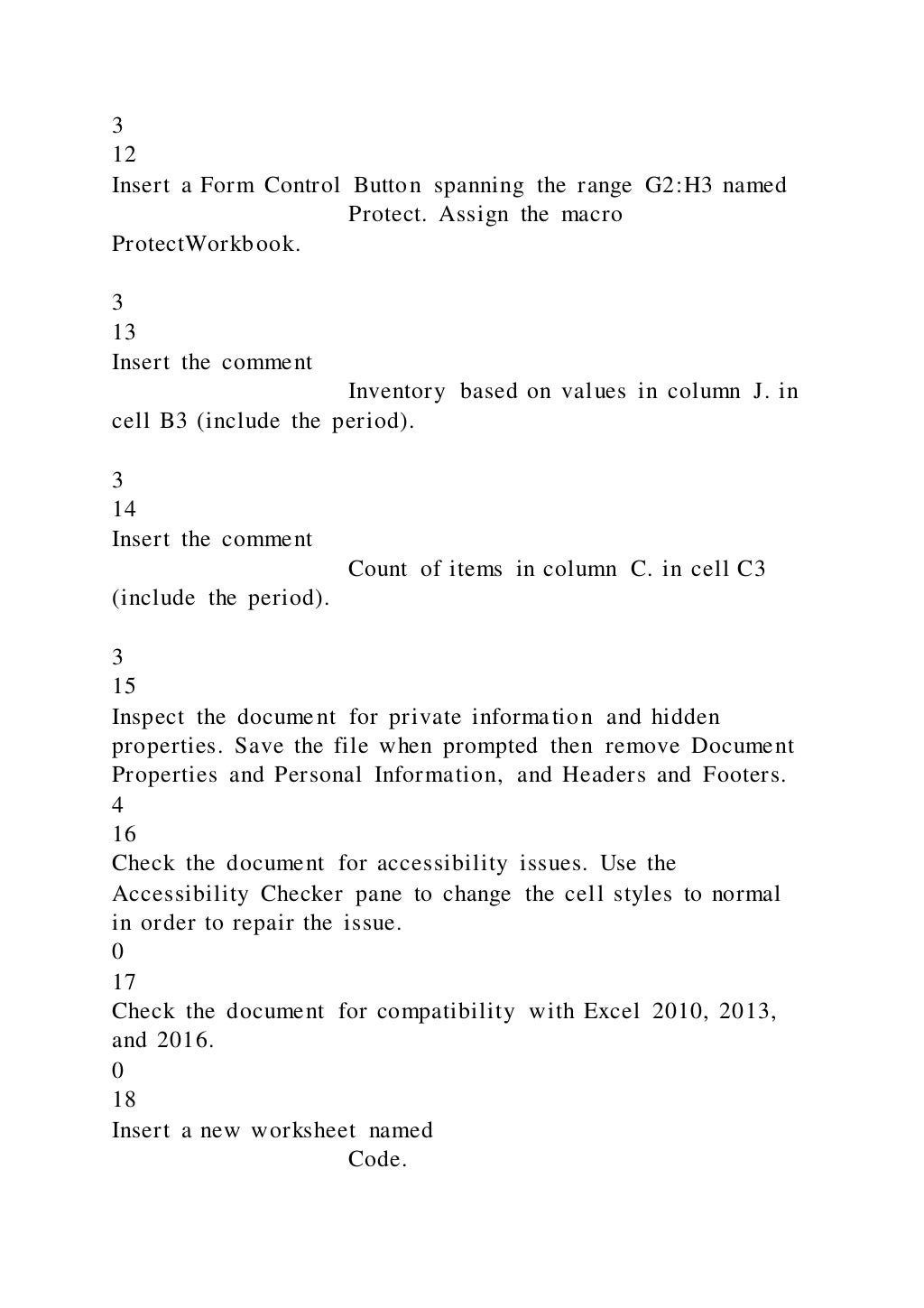
Insert a Form Control Button spanning cells F2:F3 named
Unprotect. Assign the Unprotect macro to
the newly created Control Button.
3
12
Insert a Form Control Button spanning the range G2:H3 named
Protect. Assign the macro
ProtectWorkbook.
3
13
Insert the comment
Inventory based on values in column J. in
cell B3 (include the period).
3
14
Insert the comment
Count of items in column C. in cell C3
(include the period).
3
15
Inspect the document for private information and hidden
properties. Save the file when prompted then remove Document
Properties and Personal Information, and Headers and Footers.
4
16
Check the document for accessibility issues. Use the
Accessibility Checker pane to change the cell styles to normal
in order to repair the issue.
0
17
Check the document for compatibility with Excel 2010, 2013,
and 2016.
0
18
Insert a new worksheet named
Code.
2
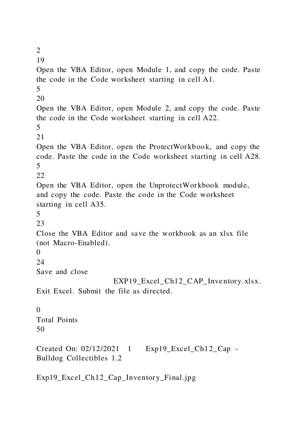
19
Open the VBA Editor, open Module 1, and copy the code. Paste
the code in the Code worksheet starting in cell A1.
5
20
Open the VBA Editor, open Module 2, and copy the code. Paste
the code in the Code worksheet starting in cell A22.
5
21
Open the VBA Editor, open the ProtectWorkbook, and copy the
code. Paste the code in the Code worksheet starting in cell A28.
5
22
Open the VBA Editor, open the UnprotectWorkbook module,
and copy the code. Paste the code in the Code worksheet
starting in cell A35.
5
23
Close the VBA Editor and save the workbook as an xlsx file
(not Macro-Enabled).
0
24
Save and close
EXP19_Excel_Ch12_CAP_Inventory.xlsx.
Exit Excel. Submit the file as directed.
0
Total Points
50
Created On: 02/12/2021 1 Exp19_Excel_Ch12_Cap -
Bulldog Collectibles 1.2
Exp19_Excel_Ch12_Cap_Inventory_Final.jpg
Exp19_Excel_App_Cap_Comp_Tech_Store_InstructionsGrader -

Exp19_Excel_App_Cap_Comp_Tech_Store_InstructionsGrader -

  • 1.
    Exp19_Excel_App_Cap_Comp_Tech_Store_Instructions.docx Grader - InstructionsExcel 2019 ProjectExp19_Excel_App_Cap_Comp_Tech_Store Project Description: After graduating from college, you and three of your peers founded the software company TechStore Unlimited (TSU). TSU provides an online market place that fosters business to business (B2B), business to consumer (B2C), and consumer to consumer sales (C2C). As one of the company’s principal owners, you have decided to compile a report that details all aspects of the business, including: employee payroll, facility management, sales data, and product inventory. To complete the task you will duplicate existing formatting, import data from an Access database, utilize various conditional logic functions, complete an amortization table, visualize data with PivotTables and Power Maps, connect and transform several external data sources, and lastly you will inspect the workbook for issues. Steps to Perform: Step Instructions Points Possible 1 Start Excel. Open Exp19_Excel_AppCapstone_Comp.xlsx. Grader has automatically added your last name to the beginning of the filename. 0 2 Fill the range A1:E1 from the Employee_Info worksheet across all worksheets, maintaining the formatting. 1.5 3
  • 2.
    Make the New_Constructionworksheet active and create Range Names based on the data in the range A6:B9. 1.5 4 Ungroup the worksheets and ensure the Employee_Info worksheet is active. Click cell G6 and enter a nested logical function that calculates employee 401K eligibility. If the employee is full time (FT) and was hired before the 401k cutoff date 1/1/19, then he or she is eligible and Y should be displayed, non-eligible employees should be indicated with a N. Be sure to utilize the date located in cell H3 as a reference in the formula. Use the fill handle to copy the function down completing the range G6:G25. 2.5 5 Apply conditional formatting to the range G6:G25 that highlights eligible employees with Green Fill with Dark Green text. Eligible employees are denoted with a Y in column G. 1.5 6 Create a Data Validation list in cell J7 based on the employee IDs located in the range A6:A25. Add the Input Message Select Employee ID and use the Stop Style Error Alert. 1.5 7 Enter a nested INDEX and MATCH function in cell K7 that examines the range B6:H25 and returns the corresponding employee information based on the match values in cell J7 and cell K6. Note K6 contains a validation list that can be used to select various lookup categories. Use the Data Validation list in cell J7 to select Employee_ID 31461 and select
  • 3.
    Salary in cellK6 to test the function. 2 8 Enter a conditional statistical function in cell K14 that calculates the total number of PT employees. Use the range E6:E25 to complete the function. 1.5 9 Enter a conditional statistical function in cell K15 that calculates the total value of PT employee salaries. Use the range E6:E25 to complete the function. 1.5 10 Enter a conditional statistical function in cell K16 that calculates the average value of PT employee salaries. Use the range E6:E25 to complete the function. 1.5 11 Enter a conditional statistical function in cell K17 that calculates the highest PT employee salary. Use the range E6:E25 to complete the function. 1.5 12 Apply Currency Number Format to the range K15:K17. 0.5 13 Click cell K11 and type
  • 4.
    FT. Click cellA28 and type Full Time Employees. 0.5 14 Use the Format Painter to apply the formatting from the cell A3 to the range A28:B28. 0.5 15 Use Advanced Filtering to restrict the data to only display FT employees based on the criteria in the range K10:K11. Place the results in cell A29. 1.5 16 Enter a database function in cell K18 to determine the total number of FT employees. To complete the function use the range A5:H25 as the database argument, cell E5 for the field, and the range K10:K11 for the criteria. 1.5 17 Enter a database function in cell K19 to determine the total value of FT employee salaries. To complete the function use the range A5:H25 as the database argument, cell H5 for the field, and the range K10:K11 for the criteria. 1.5 18 Enter a database function in cell K20 to determine the average FT employee salary. To complete the function use the range A5:H25 as the database argument, cell H5 for the field, and the range K10:K11 for the criteria. 1.5 19 Enter a database function in cell K21 to determine the highest FT salary. To complete the function use the range A5:H25 as the database argument, cell H5 for the field, and the range K10:K11 for the criteria.
  • 5.
    1.5 20 Format the rangeK19:K21 with Currency Number Format. 0.5 21 Ensure that the New_Construction worksheet is active. Use Goal Seek to reduce the monthly payment in cell B6 to the optimal value of $8000. Complete this task by changing the Loan amount in cell E6. 2.5 22 Create the following three scenarios using Scenario Manager. The scenarios should change the cells B7, B8, and E6. Good B7 = .0312 B8 = 5 Most Likely B7 = .0575 B8 = 5 Bad B7 = .0625 B8 = 3 Create a Scenario Summary Report based on the value in cell B6. Format the new report appropriately and reorder the worksheets so the Scenario Summary worksheet appears as the
  • 6.
    last worksheet inthe workbook. 4.5 23 Ensure that the New_Construction worksheet is active. Enter a reference in cell B12 to the beginning loan balance and enter a reference in cell C12 to the payment amount. 1 24 Use the IPMT function in cell D12 to calculate the interest paid for the first payment of the loan. Use the information in the loan details section (E6:E9) of the worksheet to locate the required inputs for the function. Be sure to use the appropriate absolute, relative, or mixed cell references. All results should be formatted as positive numbers. 2.5 25 Enter a formula in cell E12 based on the payment and loan details that calculates the amount of principal paid on the first payment. The principal is the payment - interest. Be sure to use the appropriate absolute, relative, or mixed cell references. 2.5 26 Enter a formula in cell F12 to calculate the remaining balance after the current payment. The remaining balance is calculated by subtracting the principal payment from the balance in column B. 2.5 27 Use the CUMIPMT function in cell G12 to calculate the cumulative interest paid on the first payment. Use the loan details information (E6:E9) as needed for inputs. Be sure to use the appropriate absolute, relative, or mixed cell references. All results should be formatted as positive values. 2.5 28
  • 7.
    Enter a functionin cell H12 based on the payment and loan details that calculates the amount of cumulative principal paid on the first payment. Be sure to use the appropriate absolute, relative, or mixed cell references. All results should be formatted as positive numbers. 2.5 29 Enter a reference to the remaining balance of payment 1 in cell B13. Use the fill handle to copy the functions created in the prior steps down to complete the amortization table. Expand the width of columns D:H as needed. 2.5 30 Use PowerQuery to connect and open the Orders table in the eApp_Cap_Orders.accdb database. Use the Query editor to format column A with Date number format and load the table. Rename the worksheet Orders. 3 31 Adapt the previous step to connect and load the Warehouse table. 1.5 32 Connect to, but don't load the Inventory table from the eApp_Cap_Orders.accdb database. 0 33 Create the following relationships. Relationship 1 Table Name Inventory
  • 8.
    Column (Foreign) Warehouse Table Warehouse Column (Primary) Warehouse Relationship2 Table Orders Column (Foreign) Item_Number Table Inventory Column (Primary) Item_Number 3 34 Use PowerPivot to create a blank PivotTable on a new worksheet. Add the following fields to the PivotTable. Rows Warehouse: Location Warehouse: Warehouse Inventory: Item_Number Values Inventory: Current_Inventory Inventory: Total_Value
  • 9.
    4 35 Insert a Slicerbased on Warehouse. Place the upper left corner of the Slicer inside the borders of cell F3. 1.5 36 Create a 3D PowerMap that displays the location of all warehouses based on the City geographic type. Rename the worksheet Inventory. 1 37 Make the Orders worksheet active. Use the Data Analysis ToolPak to output Summary statistics starting in cell G3. The statistics should be based on the quantity of orders located in the range E1:E50. Be sure to include column headings in the output. 1.5 38 Record a macro using the Macro Recorder named Sort. When activated, the macro should sort the Orders table in ascending order by date. Open the newly created module in the Visual Basic Editor and copy the code in Module1. Paste the code starting in cell A1 on the Code worksheet. 2.5 39 On the Orders worksheet, insert a Form Control button labeled Sort in the range G21:I24 and assign the Sort macro. 2 40 Use the Accessibility Checker to inspect for issues. Once
  • 10.
    located, make thefollowing changes to alleviate the issues. Warehouse worksheet Change Table Style to none. Orders worksheet Change Table Style to none. Employee_Info worksheet Change Font Color to Black, Text 1 New_Construction worksheet Change Font Color to Black, Text 1 Save the file Exp19_Excel_AppCapstone_Comp.xlsx. Exit Excel. Submit the file as directed. 1 Total Points 70 Created On: 05/05/2022 1 Exp19_Excel_App_Cap_Comp - Tech Store 1.6 Whiting_Exp19_Excel_AppCapstone_Comp.xlsx Employee_InfoTech Store UnlimitedEmployee Information401K Cut Off1/1/19Employee_IDStart_DateFirst_NameLast_NameTypeDe pendents401k EligibleSalaryEmployee Lookup314612/1/17NelsonGailFT1$ 125,000.00Employee_IDDependents567688/19/20LopezVivianF T4$ 100,000.00314281/8/17RamseyMatthewFT0$ 110,000.00462742/2/17StevensonBeverlyFT3$ 85,000.00Employee LookupFilter302614/29/20SmithPeterFT0$ 95,000.00Employee_IDTypeDependentsSalary434821/21/19Kell
  • 11.
    eyEmilyPT2$ 18,864.00886965/1/21CarrollPhyllisPT3$ 23,722.00650301/28/18HuntBarbaraPT0$ 14,966.00Employee Statistics9867412/29/18AustinMelaniePT4$18,751.00# PT9806510/14/20SnyderJeanPT1$ 18,875.00Total PT Salaries800876/4/20MorrisSuzannePT3$ 11,513.00Average PT Salary798866/15/18GibsonGeraldinePT0$ 20,044.00Highest PT Salary6440111/3/21GrahamVickiPT3$ 10,354.00# FT7292212/15/21WatsonMarilynPT4$ 11,049.00Total FT Salaries908715/30/19SimpsonTroyPT3$ 24,010.00Average FT Salary399481/14/20BarberAaronPT4$ 11,156.00Highest FT Salary4072512/7/20MoralesBrittanyPT3$ 23,142.00429881/31/19BlairCynthiaPT3$ 12,105.00404994/13/18JenningsDoloresPT0$ 24,905.00282534/29/18CarrollHowardPT3$ 10,663.00 New_ConstructionFacility Amortization TablePayment DetailsLoan DetailsPayment$8,647.55Loan$450,000.00APR5.75%Periodic Rate0.479%Years5# of Payments60Pmts per Year12Payment NumberBeginning BalancePayment AmountInterest PaidPrincipal RepaymentRemaining BalanceCumulative InterestCumulative Principal123456789101112131415161718192021222324252627 28293031323334353637383940414243444546474849505152535 4555657585960Totals$ - 0$ - 0 Code Exp19_Excel_App_Cap_Comp_Tech_Store_final_result.jpg eApp_Cap_Orders.accdbItem_NumberUnit_CostWarehouseCurr ent_InventoryTotal_Value1112.0¤ 819.00C274.0¤ 224,406.0012 32.0¤ 318.00A149.0¤ 47,382.001265.0¤ 461.00C146.0¤ 67,306. 001304.0¤ 381.00A145.0¤ 55,245.001329.0¤ 903.00C44.0¤ 39,7 32.001464.0¤ 564.00C47.0¤ 26,508.001611.0¤ 688.00A60.0¤ 41 ,280.001648.0¤ 502.00C270.0¤ 135,540.002007.0¤ 502.00C251. 0¤ 126,002.002079.0¤ 812.00C227.0¤ 184,324.002130.0¤ 263.0 0A36.0¤ 9,468.002496.0¤ 680.00C153.0¤ 104,040.002583.0¤ 45
  • 12.
    4.00B96.0¤ 43,584.003411.0¤ 186.00A2.0¤372.003464.0¤ 402. 00D225.0¤ 90,450.003706.0¤ 766.00D63.0¤ 48,258.003939.0¤ 7 44.00A27.0¤ 20,088.004697.0¤ 861.00B143.0¤ 123,123.005089. 0¤ 249.00E300.0¤ 74,700.005160.0¤ 592.00B135.0¤ 79,920.005 421.0¤ 930.00A157.0¤ 146,010.005824.0¤ 852.00B98.0¤ 83,496 .005906.0¤ 872.00B262.0¤ 228,464.006076.0¤ 198.00A75.0¤ 14 ,850.006257.0¤ 526.00A253.0¤ 133,078.006263.0¤ 792.00B66.0 ¤ 52,272.006466.0¤ 594.00C36.0¤ 21,384.006685.0¤ 351.00B26 7.0¤ 93,717.006871.0¤ 742.00B231.0¤ 171,402.006884.0¤ 197. 00B126.0¤ 24,822.007082.0¤ 379.00A96.0¤ 36,384.007333.0¤ 1 93.00A43.0¤ 8,299.007361.0¤ 481.00A241.0¤ 115,921.007508.0 ¤ 488.00A10.0¤ 4,880.007553.0¤ 622.00A31.0¤ 19,282.007636. 0¤ 57.00B15.0¤ 855.007640.0¤ 277.00A23.0¤ 6,371.007664.0¤ 847.00C2.0¤ 1,694.008107.0¤ 666.00D139.0¤ 92,574.008342.0¤ 16.00A197.0¤ 3,152.008368.0¤ 320.00B189.0¤ 60,480.008547. 0¤ 590.00A111.0¤ 65,490.008611.0¤ 591.00D36.0¤ 21,276.0093 79.0¤ 28.00A217.0¤ 6,076.009398.0¤ 148.00C204.0¤ 30,192.00 9423.0¤ 393.00C104.0¤ 40,872.009443.0¤ 982.00A185.0¤ 181,6 70.009482.0¤ 661.00E252.0¤ 166,572.009744.0¤ 716.00E65.0¤ 46,540.009824.0¤ 769.00B47.0¤ 36,143.00DateOrder_IDItem_N umberSupplier_NumberQuantity2020-01- 011000.06884.05446.011.02020-01- 081001.09482.05446.016.02020-01- 141002.03939.04165.09.02020-01- 251003.07333.03437.021.02020-01- 271004.02583.05446.03.02020-02- 071005.06871.03437.011.02020-02- 221006.09423.07741.011.02020-03- 041007.05421.05446.023.02020-03- 071008.07333.05446.016.02020-03- 121009.09398.05446.08.02020-03- 231010.08107.03437.022.02020-03- 261011.07082.04165.021.02020-04- 031012.08342.03437.022.02020-04- 041013.07333.05446.03.02020-04- 091014.01329.07741.019.02020-04-
  • 13.
    131015.09482.03437.013.02020-04- 281016.09824.03437.09.02020-05- 031017.07361.03437.022.02020-05- 041018.09423.07741.019.02020-05- 071019.07640.03437.023.02020-05- 291020.06466.07741.011.02020-06- 011021.02130.05446.022.02020-06- 031022.02583.07741.017.02020-07- 061023.06871.07741.021.02020-07- 281024.01304.03437.08.02020-08- 161025.07553.03437.02.02020-08- 191026.07664.05446.011.02020-08- 261027.09423.05446.023.02020-09- 041028.06685.03437.015.02020-09- 091029.02007.05446.016.02020-09- 131030.01304.04165.017.02020-09- 191031.06263.03437.022.02020-09- 201032.02496.03437.012.02020-09- 301033.09379.05446.08.02020-10- 121034.07333.07741.012.02020-10- 141035.05824.07741.023.02020-10- 171036.06257.03437.017.02020-10- 241037.09482.05446.09.02020-10- 301038.09398.07741.03.02020-11- 021039.05824.04165.016.02020-11- 141040.09443.03437.015.02020-11- 251041.07640.05446.01.02020-12- 021042.05421.05446.06.02020-12- 161043.03464.03437.015.02020-12- 191044.06257.05446.019.02020-12- 221045.05089.04165.02.02020-12- 291046.09824.03437.022.02020-12- 301047.05824.07741.023.02020-12- 311048.03706.04165.08.0WarehouseLocationAChicago, IllinoisBIndianapolis, IndianaCCleveland, OhioDDenver, ColoradoEPortland,Oregon
  • 14.
    Whiting_Exp19_Excel_Ch11_Cap_Donors.xlsx DonorsLook Up AreaFormulasSummaryDonorID:ART-39Cell B3Total Donations:Donor Position:Cell B4Average donation:Donor Name:Cell D8Total donors:Donor Amount:Cell K2CollegeCollege IDDonor IDNew Donor IDFull NameLast NameAddressCityStateCollege/SchoolDonationENGINEERING 15Schneider, Dedrick1243 W Abbey Rd,Columbus,OH5,000BUSINESS25Beauclair, Oliver34 E Affinity Dr,Cincinnati,OH7,500BUSINESS27Flores, Adrian912 E Julien Circle,Akron,OH10,000ART45Wang, Shan2945 N Country Club Rd,Chicago Heights,IL3,500ENGINEERING22Schafer, Elysia259 S Wadsbury Dr,Cincinnati,OH4,000ART39Romero, Samantha123 W Lincoln Ave,Dayton,OH6,000ART12Mikhailov, Jon342 S Newton Dr,Columbus,OH750BUSINESS14Jaundreau, Hunter64 E 111th Place,Chicago,IL500ENGINEERING18Kato, Eiji41 W Eaton Drive,Toledo,OH1,250ENGINEERING23Schroder, Genevie6124 N Odelle Dr,Akron,OH3,000ART24Diaz, Sergio142 S Elm Street,Erie,PA1,255BUSINESS31Lamoureux, Lucas3415 N Saddlewood Dr,Toledo,OH3,000ART36Acosta, Jaime1490 S Alcove Way,Pittsburgh,PA855ART42Ishikawa, Chie4152 E Dalbren Ln,Cincinnati,OH6,500BUSINESS44Kruger, Alfonso641 W Banbury Dr,Toledo,OH2,500ART38Normandeau, Amelia45 E Blackstone Court,Detroit,MI5,555ENGINEERING52Cabrera, Mia923 W Haldy Rd,Columbus,OH3,545BUSINESS53Fernandez, Isabella641 S Caiser Court,San Francisco,CA4,210BUSINESS49Wright, Jerri64 W Garden Court,Bowling Green,OH900ENGINEERING47Friedrich, Ava15 E Oak Hill Drive,Anaheim,CA950ENGINEERING26Byram, Emma324 E Deer Valley Drive,Park City,UT11,000ART46Renault, Linden3434 E Wallhaven Circle,Akron,OH12,500BUSINESS55Sanchez, Caleb25 W
  • 15.
    Catherine Street,Ann Arbor,MI2,355ART41Zhang,Jun3914 McCartney Rd,Youngstown,OH900ENGINEERING33Deneau, Abigail345 N Cobb Place,Detroit,MI1,600BUSINESS58Walker, Mitchell1850 N Lelanford Cir,Bowling Green,OH655ART34Perez, Tina45 E Keyes Ave,Cleveland,OH6,545ENGINEERING58Morgan, Terry1200 E. Monticello Blvd,Cleveland,OH750 Exp19_Excel_Ch11_Cap_Donors_Instructions.docx Grader - Instructions Excel 2019 ProjectExp19_Excel_Ch11_Cap_Donors Project Description: You are a development officer for a state university. As an officer, you manage a portfolio of important donors who contribute financially to different areas within the university. You categorize the donors based on the college or school for which they want their donations associated. You recently downloaded the portfolio to an Excel workbook. Based on the way the data downloads from the main database, you want to format the text for readability and to make it easier for you to analyze. In addition, you will create an advanced filter to review a list of donors for a particular college or school. Finally, you want to create a look up area to look up data for a specific donor and create a summary section. Steps to Perform: Step Instructions Points Possible 1 Start Excel. Download and open the file named Exp19_Excel_Ch11_Cap_Donors.xlsx. Grader has automatically added your last name to the beginning of the filename. 0 2
  • 16.
    The first columndisplays the name of the college or school (such as ART or BUSINESS) associated with each. You want to assign a three-character code for each college and use that code to attach to existing donor IDs to create a unique field. In cell B8, insert the LEFT function to extract the first three characters from the college name in cell A8. Copy the function to the range B9:B35. 2.5 3 You now want to combine the college ID and donor ID. In cell D8, insert the CONCAT function to combine the college ID in cell B8 with the donor ID in cell C8 with a hyphen between the two text strings. Copy the function to the range D9:D35. 2.5 4 In cell J8, insert a text function that displays the college name from cell A8 with just the first letter capitalized, such as Engineering. Copy the function to the range J9:J35. 2.5 5 The Full Name column displays last and first names of the donors. You want to display last names only in a separate column. In cell F8, type Schneider and use Flash Fill to fill in the last names for the donors in the range F9:F35.
  • 17.
    2.5 6 The Address columncontains street addresses, city names, and state abbreviations. To manage the address list better, you will separate the data into three columns. Select the addresses in the range G8:G35 and convert the text to columns, separating the data at commas . 5 7 The top-left section of the spreadsheet is designed to be able to enter a donor’s ID, such as ENG-15, and look up that person’s position in the list, display the donor’s full name, and display the amount donated this year. The first step is to identify the position number of the donor ID. In cell B3, insert the MATCH function to look up the donor ID in cell B2, compare it to the list in the range D8:D35, and then return the donor’s position within the list. 3 8 Now you are ready to use the position number as an argument within the INDEX function. In cell B4, insert an INDEX function that uses the range D8:K35, looks up the row position number from the MATCH function result, and then uses the column position number for Full Name. 3 9 In cell B5, insert an INDEX function that uses the range D8:K35, looks up the row position number from the MATCH function result, and then uses the column position number for Donation. 3
  • 18.
    10 You want toformat the results of the INDEX function. Format the value in cell B5 as Accounting Number Format with zero decimal places. 1.5 11 To analyze the donor records, you are ready to create criteria and output ranges. You will enter conditions to find records for donors to the College of Business who donated $1,000 or more. Copy the range A7:K7 to cell A38 to create the column labels for the criteria range. Type Business in cell J39 and >=1000 in cell K39. 3.5 12 You are ready to create the output area and perform the advanced filter. Copy the column labels to cell A42. Perform the advanced filter by copying the records to the output area. 3 13 Now that you created a copy of the records meeting the conditions, you are ready to enter database functions in the Summary area. In cell K2, insert the database function to total the value of the donations for the records that meet the conditions in the criteria range. 3 14 In cell K3, insert the database function to calculate the average
  • 19.
    donation for therecords that meet the conditions in the criteria range. 3 15 In cell K4, insert the database function to count the number of records that meet the conditions in the criteria range. 3 16 Format the range K2:K3 with Accounting Number Format with zero decimal places. Format cell K4 with Comma Style with zero decimal places. 1.5 17 You want to use the FORMULATEXT function to display the functions. In cell G2, insert the FORMULATEXT function to display the formula stored in cell B3. In cell G3, insert the FORMULATEXT function to display the formula stored in cell B4. In cell G4, insert the FORMULATEXT function to display the formula stored in cell D8. In cell G5, insert the FORMULATEXT function to display the formula stored in cell K2. 6 18 Create a footer with your name on the left side, the sheet name code in the center, and the file name code on the right side of the worksheet. 1.5 19 Save and close Exp19_Excel_Ch11_Cap_Donors.xlsx. Exit Excel. Submit the file as directed. 0
  • 20.
    Total Points 50 Created On:06/12/2020 1 Exp19_Excel_Ch11_Cap - Donors 1.0 Exp19_Excel_Ch11_Cap_Donors_final_result.jpg Whiting_EXP19_Excel_Ch12_Cap_Inventory.xlsx Inventory ListINVENTORY LISTTOTAL INVENTORY VALUE:INVENTORY ITEMS:BIN COUNT:INVENTORY PICK LISTBIN LOOKUP$4,649.00116SKUDESCRIPTIONBIN #LOCATIONUNITQTYREORDER QTYCOSTINVENTORY VALUEREORDERSP7875Item 1T345Row 2, slot 1Each2010$30.00$600.00TR87680Item 2T345Row 2, slot 1Each3015$40.00$1,200.00MK676554Item 3T5789Row 1, slot 1Each105$5.00$50.00YE98767Item 4T9876Row 3, slot 2Box (10 ct)4010$15.00$600.00XR23423Item 5T098Row 3, slot 1Each1210$26.00$312.00PW98762Item 6T345Row 2, slot 1Each710$50.00$350.00ReorderBM87684Item 7T349Row 1, slot 2Each105$10.00$100.00BH67655Item 8T5789Row 1, slot 1Each1910$3.00$57.00WT98768Item 9T9875Row 2, slot 2Package (5 ct)2030$14.00$280.00ReorderTS3456Item 10T349Row 1, slot 2Each158$60.00$900.00WDG123Ite m 11T349Row 1, slot 2Each2515$8.00$200.00 INVENTORY PICK LIST/xl/drawings/drawing1.xml#'Inventory%20Pick%20List'!A 1 BIN LOOKUP/xl/drawings/drawing1.xml#'Bin%20Lookup'!A1 Inventory Pick ListINVENTORY PICK LISTINVENTORY LISTORDER #SKUPICK QTYQTY AVAILABLEITEM DESCRIPTIONUNITBIN #LOCATIONTP001-1SP7875320Item 1EachT345Row 2, slot 1TP001-1YE98767140Item 4Box (10 ct)T9876Row 3, slot 2TP001-1BM87684210Item 7EachT349Row 1, slot 2TP001-1TS3456615Item
  • 21.
    10EachT349Row 1, slot2TP001-1MK676554310Item 3EachT5789Row 1, slot 1 INVENTORY LIST/xl/drawings/drawing2.xml#'Warehouse%20Inventory%20L ist'!A1 CLEAR PICK LIST Bin LookupBIN LOOKUPINVENTORY LISTBIN #DESCRIPTIONLOCATIONWIDTHHEIGHTLENGTHT345Lar ge binRow 2, slot 1501010T5789Small binRow 1, slot 12555T9876Large binRow 3, slot 2501010T098Medium binRow 3, slot 130710T349Small binRow 1, slot 22555T5789Large binRow 4, slot 5501010T9875Large binRow 2, slot 2501010 INVENTORY LIST/xl/drawings/drawing3.xml#'Warehouse%20Inventory%20L ist'!A1 Exp19_Excel_Ch12_Cap_Bulldog_Collectibles_Instructions.doc x Grader - Instructions Excel 2019 ProjectExp19_Excel_Ch12_Cap_Bulldog_Collectibles Project Description: You are the operations manager for Bulldog collectables, a small start-up company that deals with sports memorabilia. As you prepare to document your inventory, you decide to utilize a template to save time. To complete this task, you will create a worksheet based on an Office.com template; you will also use the Macro Recorder and Visual Basic for Application to automate sorting and calculations within the workbook. Steps to Perform: Step Instructions Points Possible 1 Start Excel. Download and open the file named EXP19_Excel_Ch12_Cap_Inventory.xlsx. Grader has automatically added your last name to the beginning
  • 22.
    of the filename. 0 2 Deletethe Inventory Pick List and Bin Lookup worksheets. 1.5 3 Delete the INVENTORY PICK LIST and BIN LOOKUP icons located respectively in cells E2 and F2. Then Clear all existing Data Validation in the range A1:K15. 1.5 4 Delete the values in the range B5:J15. 1.5 5 Record a macro named Sort, be sure to use relative references. Ensure the macro sorts the data in the table in ascending order based on SKU (column A). Stop the Macro Recorder and Save the workbook as a Macro-Enabled Template. 0 6 Create a form control button that spans the cell E2:E3. Assign the Sort macro and edit the button text to Sort. 3 7 Use the VBA Editor to create a new module. Type the following VBA code to create a custom Inventory Value function then save and exit the VBA Editor:
  • 23.
    Function InventoryValue (QTY, COST)InventoryValue= QTY * COST 0 8 Click cell J5 and use the newly created InventoryValue function to calculate the value of the inventory for each item in column I. 4.5 9 Use the VBA Editor to create a new module named ProtectWorkbook. Type the following VBA statements to create the sub procedure. Sub ProtectWorkbook‘Protect workbook using the password eXploringWorksheets("Inventory List").Protect Password:="eXploring" 0 10 Insert a new module named UnprotectWorkbook. Type the following VBA statements to create the sub procedure and then save and exit the VBA Editor: Sub UnprotectWorkbook()‘Unprotect workbook using the password eXploringWorksheets("Inventory List").Unprotect Password:="eXploring" 0 11 Insert a Form Control Button spanning cells F2:F3 named Unprotect. Assign the Unprotect macro to the newly created Control Button.
  • 24.
    3 12 Insert a FormControl Button spanning the range G2:H3 named Protect. Assign the macro ProtectWorkbook. 3 13 Insert the comment Inventory based on values in column J. in cell B3 (include the period). 3 14 Insert the comment Count of items in column C. in cell C3 (include the period). 3 15 Inspect the document for private information and hidden properties. Save the file when prompted then remove Document Properties and Personal Information, and Headers and Footers. 4 16 Check the document for accessibility issues. Use the Accessibility Checker pane to change the cell styles to normal in order to repair the issue. 0 17 Check the document for compatibility with Excel 2010, 2013, and 2016. 0 18 Insert a new worksheet named Code.
  • 25.
    2 19 Open the VBAEditor, open Module 1, and copy the code. Paste the code in the Code worksheet starting in cell A1. 5 20 Open the VBA Editor, open Module 2, and copy the code. Paste the code in the Code worksheet starting in cell A22. 5 21 Open the VBA Editor, open the ProtectWorkbook, and copy the code. Paste the code in the Code worksheet starting in cell A28. 5 22 Open the VBA Editor, open the UnprotectWorkbook module, and copy the code. Paste the code in the Code worksheet starting in cell A35. 5 23 Close the VBA Editor and save the workbook as an xlsx file (not Macro-Enabled). 0 24 Save and close EXP19_Excel_Ch12_CAP_Inventory.xlsx. Exit Excel. Submit the file as directed. 0 Total Points 50 Created On: 02/12/2021 1 Exp19_Excel_Ch12_Cap - Bulldog Collectibles 1.2 Exp19_Excel_Ch12_Cap_Inventory_Final.jpg