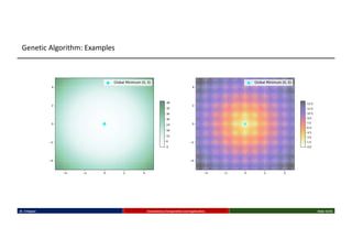
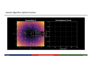
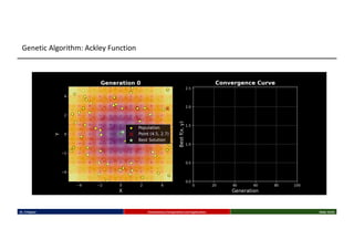
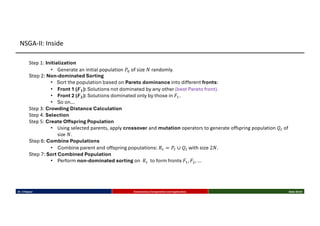
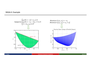
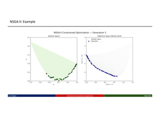
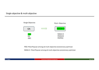
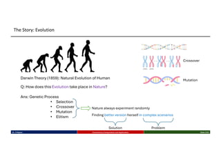
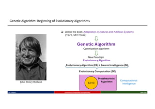
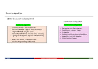
This talk introduces the fundamental principles of evolutionary computation, covering both single-objective and multi-objective optimization using Genetic Algorithms (GAs) and advanced methods such as NSGA-II. The presentation walks through the evolutionary process—selection, crossover, mutation, and elitism—and illustrates their implementation through benchmark functions like the Sphere and Ackley functions. Particular focus is given to real-world applications in business analytics, especially combinatorial optimization problems like the Travelling Salesman Problem (TSP). The discussion also highlights the scalability, flexibility, and future direction of evolutionary algorithms in the context of big data and machine learning.

1. Dr. Kanchan Rajwar
Department of Computer Science
University of Pretoria, Johannesburg, South Africa
Workshop: AI, ML and Optimization Techniques for Business Analytics
Statistical Quality Control & Operations Research Unit, Hyderabad
Indian Statistical Institute, India
Evolutionary Computation and
Application
Date: 25 May 2025

2. Dr. K Rajwar Evolutionary Computation and Application Slide 2/34
Part I: Single Objective Optimization

3. Darwin Theory (1859): Natural Evolution of Human
Q: How does this Evolution take place in Nature?
Ans: Genetic Process
• Selection
• Crossover
• Mutation
• Elitism
Crossover
Mutation
Finding better version herself in complex scenarios
Nature always experiment randomly
Solution Problem
Dr. K Rajwar Evolutionary Computation and Application Slide 3/34
The Story: Evolution

4. John Henry Holland
q Wrote the book Adaptation in Natural and Artificial Systems
(1975, MIT Press)
Genetic Algorithm
Optimization algorithm
New Paradigm
Evolutionary Algorithm
Evolutionary Algorithm (EA) + Swarm Intelligence (SI)
Evolutionary Computation (EC)
EA+SI
Metaheuristic
Algorithm Computational
Intelligence
Dr. K Rajwar Evolutionary Computation and Application Slide 4/34
Genetic Algorithm: Beginning of Evolutionary Algorithms

5. Dr. K Rajwar Evolutionary Computation and Application Slide 5/34
Genetic Algorithm
q Why do we use Genetic Algorithm?
Traditional Algorithm Non-Traditional Algorithm
• Gradient Descent - require derivate
• Newton’s Method - require Hessian matrices
• Simplex Method - only for linear
• Interior Point Methods- requires strict convexity
• Lagrangian Multipliers- requires differentiability
• Branch and Bound / Cut-not scalable
• Dynamic Programming-not scalale
• Derivative-Free Optimization
• Flexibility in Problem Types
• Scalability
• Robustness (Ill-conditioned problem)
• Adaptivity and Hybridization
• Multi-Solution Search
Evolutionary computation

6. Initialize Population
Selection
Crossover
Mutation
Elitism
Step 1
Step 2
Step 3
Step 4
Step 5
𝑂𝑏𝑗𝑒𝑐𝑖𝑣𝑒 ∶ 𝑀𝑖𝑛𝑖𝑚𝑖𝑧𝑒 𝐹 𝑋 = −20𝑒
!".$
!
"
∑#$!
%
&#
&
− 𝑒
!
'.&
∑#$!
%
'()($+&#)
+ 20 + 𝑒 𝑋 ∈ −5,5 $
Dr. K Rajwar Evolutionary Computation and Application Slide 6/34
Genetic Algorithm: Inside

7. 𝑋- = 2.6, 4.3 = [0010100110, 0100010011]
𝑋/ = −2, −3.7 = [1110000000,1101101100]
Binary (4 bits int + 6 bits frac)
Cartesian space Binary space
= [0010100110 0100010011]
= [1110000000 1101101100]
20 bits binary number
20 bits binary number
𝐹 𝑋- = 389
𝐹 𝑋/ = 1632
Dr. K Rajwar Evolutionary Computation and Application Slide 7/34
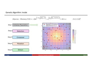
Genetic Algorithm: Initialization (Step 1)

8. Tournament selection
𝑋-
𝑋-0
𝑋1
𝑋- 𝑋/
Dr. K Rajwar Evolutionary Computation and Application Slide 8/34
Genetic Algorithm: Selection (Step 2)

9. Parent 2: X! 1110000000 1101101100
Parent 1: X# 0010100110 0100010011
1-point crossover at bit 10
Child 1 ∶ 0010100110 1101101100
Child 2 ∶ 1110000000 0100010011
Bit position 7 to flip in C1
Bit position 15 to flip in C2
1110000000 0100000011
0010100010 1101101100
Mutation
Dr. K Rajwar Evolutionary Computation and Application Slide 9/34
Genetic Algorithm: Crossover & Mutation (Step 3 & 4)

10. 𝑃! (2.6, 4.3) (0010100110, 0100010011) (0010100010, 1101101100) (2.53, −2.31) 𝐶!
𝑃" (−2.0, −3.7) (1110000000, 1101101100) (1110000000, 0100000011) (−2.00, 4.04) 𝐶"
Parents Final Child
Q: Now weather child survive?
A : If fitness of child is better than parents then child will survive
Fitness better !
𝑌𝑒𝑠 𝑆𝑢𝑟𝑣𝑖𝑏𝑒
𝑁𝑜 𝑁𝑜 𝑠𝑢𝑟𝑣𝑖𝑏𝑒
Elitism
Dr. K Rajwar Evolutionary Computation and Application Slide 10/34
Genetic Algorithm: Elitism (Step 5)
𝐹 𝑃- = 389
𝐹 𝑃$ = 1632
𝐹 𝐶- = 268
𝐹 𝐶$ = 2217

11. qOptimization Problem: Simple to Complex
𝐹- 𝑋 = C
23-
4
𝑥2
𝐹$ 𝑋 = −20𝑒
!".$
!
"
∑#$!
%
&#
&
− 𝑒
!
'.&
∑#$!
%
'()($+&#)
+ 20 + 𝑒
𝐸𝑥𝑎𝑚𝑝𝑙𝑒 1: 𝑆𝑝ℎ𝑒𝑟𝑒 𝑓𝑢𝑛𝑐𝑡𝑖𝑜𝑛 𝐸𝑥𝑎𝑚𝑝𝑙𝑒 2: 𝐴𝑐𝑘𝑙𝑒𝑦 𝑓𝑢𝑛𝑐𝑡𝑖𝑜𝑛
Dr. K Rajwar Evolutionary Computation and Application Slide 11/34
Genetic Algorithm: Examples

12. Dr. K Rajwar Evolutionary Computation and Application Slide 12/34
Genetic Algorithm: Examples

13. Dr. K Rajwar Evolutionary Computation and Application Slide 13/34
Genetic Algorithm: Sphere Function

14. Dr. K Rajwar Evolutionary Computation and Application Slide 14/34
Genetic Algorithm: Ackley Function

15. Dr. K Rajwar Evolutionary Computation and Application Slide 15/34
Genetic Algorithm: Fact
• More than 100 variants of GA available in literature
• Extensively employed in industry such as electrical engineering, AI-ML industry, port polio optimization
• More than 90000 GS citation still date

16. Part II: Multi-Objective Optimization
Dr. K Rajwar Evolutionary Computation and Application Slide 17/34

17. q Single objective optimization problem can be tackled by GA .
q What is about Multi-Objective Optimization Problem?
GA Non-Shorting Genetic Algorithm
(NSGA)
NSGA-II
Single objective Multi-Objective
1975 1994 2002
2002
• NSGA-II : Most popular among all muti-objective optimization algorithms
Kalyanmoy
Deb
Dr. K Rajwar Evolutionary Computation and Application Slide 17/34
NSGA II: The Beginning

18. q But what is Multi-objective optimization problem?
Cost (Rs)
Comfort
(%)
Pareto-optimal
front
20%
4 Lakh 25 Lakh 60 Lakh
80%
A
B
C
D
E
F
G
H
I
J
50%
F: (25 Lakh, 70% comfort)
J : (25 Lakh, 50% comfort)
J is dominated by F
F is not dominated (Pareto Solution)
Pareto Front: collation of all pareto solutions
Objective: Minimize Cost
Maximize Comfort
70%
Dr. K Rajwar Evolutionary Computation and Application Slide 18/34
Multi-Objective Optimization

19. 𝐷𝑜𝑚𝑖𝑛𝑎𝑡𝑖𝑜𝑛 ∶ 𝐴 𝑠𝑜𝑙𝑢𝑡𝑖𝑜𝑛𝑠 𝑋-
𝑖𝑠 𝑠𝑎𝑖𝑑 𝑡𝑜 𝑑𝑜𝑚𝑖𝑛𝑎𝑡𝑒 𝑡ℎ𝑒 𝑜𝑡ℎ𝑒𝑟 𝑠𝑜𝑙𝑢𝑡𝑖𝑜𝑛 𝑋$
, 𝑖𝑓 𝑏𝑜𝑡ℎ 𝑐𝑜𝑛𝑑𝑖𝑡𝑖𝑜𝑛𝑠 1 𝑎𝑛𝑑 2 𝑎𝑟𝑒 𝑡𝑟𝑢𝑒:
1. 𝑋-
𝑖𝑠 𝑛𝑜 𝑤𝑟𝑜𝑠𝑒 𝑡ℎ𝑎𝑛 𝑋$
𝑖𝑛 𝑎𝑙𝑙 𝑜𝑏𝑗𝑒𝑐𝑡𝑖𝑣𝑒𝑠
2. 𝑋-
𝑖𝑠 𝑠𝑡𝑟𝑖𝑐𝑡𝑙𝑦 𝑏𝑒𝑡𝑡𝑒𝑟 𝑡ℎ𝑎𝑛 𝑋$
𝑖𝑛 𝑎𝑡 𝑙𝑒𝑎𝑠𝑡 𝑜𝑛𝑒 𝑜𝑏𝑗𝑒𝑐𝑡𝑖𝑣𝑒
𝑃𝑎𝑟𝑒𝑡𝑜 𝑓𝑟𝑜𝑛𝑡 ∶ 𝑃 = {𝑋 |𝑋 𝑖𝑠 𝑛𝑜𝑛 𝑑𝑜𝑚𝑖𝑛𝑎𝑡𝑒𝑑 𝑠𝑜𝑙𝑢𝑡𝑖𝑜𝑛 𝑖𝑛 𝑆}
𝑃𝑎𝑟𝑒𝑡𝑜 𝑠𝑜𝑙𝑢𝑡𝑖𝑜𝑛 ∶ 𝑋 𝑖𝑠 𝑝𝑎𝑟𝑒𝑡𝑜 𝑠𝑜𝑙𝑢𝑡𝑖𝑜𝑛 𝑖𝑓 𝑋 𝑖𝑠 𝑛𝑜𝑛 𝑑𝑜𝑚𝑖𝑛𝑎𝑡𝑒𝑑.
Dr. K Rajwar Evolutionary Computation and Application Slide 19/34
Multi-Objective Optimization

20. Step 1: Initialization
• Generate an initial population 𝑃" of size 𝑁 randomly.
Step 2: Non-dominated Sorting
• Sort the population based on Pareto dominance into different fronts:
• Front 1 (𝑭𝟏): Solutions not dominated by any other (best Pareto front).
• Front 2 (𝑭𝟐): Solutions dominated only by those in 𝐹-.
• So on…
Step 3: Crowding Distance Calculation
Step 4: Selection
Step 5: Create Offspring Population
• Using selected parents, apply crossover and mutation operators to generate offspring population 𝑄7 of
size 𝑁.
Step 6: Combine Populations
• Combine parent and offspring populations: 𝑅7 = 𝑃7 ∪ 𝑄7 with size 2𝑁.
Step 7: Sort Combined Population
• Perform non-dominated sorting on 𝑅7 to form fronts 𝐹-, 𝐹$, …
Dr. K Rajwar Evolutionary Computation and Application Slide 20/34
NSGA-II: Inside

21. 𝑀𝑖𝑛𝑖𝑚𝑖𝑧𝑒 𝐹- 𝑥-, 𝑥$ = −𝑥-
𝑀𝑖𝑛𝑖𝑚𝑖𝑧𝑒 𝐹$ 𝑥-, 𝑥$ = 𝑥- + 𝑥$
$
Subject to a
𝑔- 𝑋 = −𝑥-
$
+ 𝑥$ ≥ 0
𝑔$(𝑋) = −𝑥- − 2𝑥$ + 3 ≥ 0
𝑋 = 𝑥-, 𝑥$ ∈ 𝑅$
Dr. K Rajwar Evolutionary Computation and Application Slide 21/34
NSGA-II: Example

22. Dr. K Rajwar Evolutionary Computation and Application Slide 22/34
NSGA-II: Example

23. Dr. K Rajwar Evolutionary Computation and Application Slide 23/34
NSGA-II
GA
NSGA-II : Most Popular among all multi-objective evolutionary optimizer
PSO: Most Popular among all multi-objective evolutionary optimizer
PSO
DE
ABC
NSGA-III
MOEA/D
MOPSO
Single Objective Multi -Objective
Single objective & multi-objective

24. Part III: Application in Business Analytics
Dr. K Rajwar Evolutionary Computation and Application Slide 24/34

25. Optimization Model
𝑀𝑖𝑛. 𝑓 𝑋
𝑆𝑢𝑏𝑗𝑒𝑐𝑡 𝑡𝑜 f
𝑔- 𝑋 ≥ 0
𝑔$(𝑋) ≥ 0
𝑋 ≥ 0
Methods to solve
• Linear Programming
• Integer Programming
• Evolutionary Algorithm
• Metaheuristic Algorithms
Real Life Problem
Optimization in business analytics involves using mathematical models and algorithms to make data-driven
decisions that maximize efficiency, profitability, or other key metrics while minimizing costs or risks
Dr. K Rajwar Evolutionary Computation and Application Slide 25/34
Application

26. q Problem: Delivery Route Optimization
A logistics company needs to deliver goods to 10 cities (nodes) using a single delivery truck. The goal is to
minimize the total distance travelled while visiting each city exactly once and returning to the starting point.
The company wants to reduce fuel costs and delivery time.
This is a combinatorial optimization problem, where the number of possible routes (permutations) grows
factorially (10! = 36,28,800 possible routes), making exhaustive search impractical.
Dr. K Rajwar Evolutionary Computation and Application Slide 26/34
Application: Travelling Salesman Problem

27. Dr. K Rajwar Evolutionary Computation and Application Slide 27/34
Application: Travelling Salesman Problem

28. q Challenge: TSP is NP Hard problem.
q An evolutionary algorithm, like a GA, can efficiently find a near-optimal route.
q Greeter than 20 cities (Variable), traditional algorithm like Gurobi,
LPP fail to solve withing a time
Metaheuristic Algorithms
Dr. K Rajwar Evolutionary Computation and Application Slide 28/34
Application: Travelling Salesman Problem

29. Mathematical Formulation (Symmetric TSP)
Let:
• 𝑛: number of cities
• 𝑉 = {1,2, … , 𝑛}: set of cities
• 𝑑28: distance (or cost) between city 𝑖 and city 𝑗, with 𝑑22 = 0, and 𝑑28 = 𝑑82
• 𝑥28 ∈ {0,1} : binary variable, 1 if the path goes directly from city 𝑖 to city 𝑗, 0 otherwise
Objective Function 𝑀𝑖𝑛. 𝑓 = C
23-
4
C
83-
4
𝑑28 𝑥28
Constraints
1. Each city is entered exactly once:
2. Each city is exited exactly once:
3. No self-loop (no staying at same city):
C
23-
4
𝑥28 = 1 ∀ 𝑗 ∈ 𝑉
C
83-
4
𝑥28 = 1 ∀ 𝑖 ∈ 𝑉
𝑥28 = 0 ∀ 𝑗 ∈ 𝑉
Given
Need to find
Dr. K Rajwar Evolutionary Computation and Application Slide 29/34
Application: Travelling Salesman Problem

30. Dr. K Rajwar Evolutionary Computation and Application Slide 30/34
Application: Travelling Salesman Problem

31. Best Tour (City Names):
City_1 → City_6 → City_4 → City_9 → City_8 → City_3 → City_10 → City_7 → City_2 → City_5 → City_1
Total Distance: 291.55 km
Dr. K Rajwar Evolutionary Computation and Application Slide 31/34
Application: Travelling Salesman Problem

32. Dr. K Rajwar Evolutionary Computation and Application Slide 32/34
Application: Travelling Salesman Problem

33. q What is the future of Evolutionary computations?
Published in 2017
• Evolutionary Algorithms is powerful than alternate of Reinforcement Learning.
Big Data
Scalable Problem Solver
Trending
Evolutionary algorithm + Machine Learning
Dr. K Rajwar Evolutionary Computation and Application Slide 33/34
Evolutionary Algorithm: Trend and Future

34. THANKS
Most welcome for any question, Suggestion and collaboration
Email: kanchanrajwar1519@gmail.com