Downloaded 18 times
![Enterprise Applications in the Cloud:
Analysis of Pay-per-use Plans
Leonid Grinshpan, Oracle Corporation (www.oracle.com)
The Cloud-computing paradigm is attractive to businesses not only because of its
technological, logistical, and environmental advantages over traditional IT frameworks.
For the most part its magnetic pull has its roots in economy—Clouds are also well
suited to save IT cost as they implement pay-per-use policies.
While relocating enterprise applications (EA) into the Cloud, the corporations have to
be aware of the cost associated with Cloud services and its dependence on dynamically
changing EA workloads. The same is true for Cloud providers: they have to know the
revenue derived from each hosted EA. This article provides guidance to Cloud users
and Cloud providers on cost/revenue estimates. It explores cost/revenue models for two
pay-per-use plans: pay-per-resource and pay-per-transaction. A modeling approach is
based on methodology described in the author’s book [Leonid Grinshpan. Solving
Enterprise Application Performance Puzzles: Queuing Models to the Rescue, Willey-IEEE
Press, 2012. http://www.amazon.com/Solving-Enterprise-Applications-Performance-
Puzzles/dp/1118061578/ref=ntt_at_ep_dpt_1].
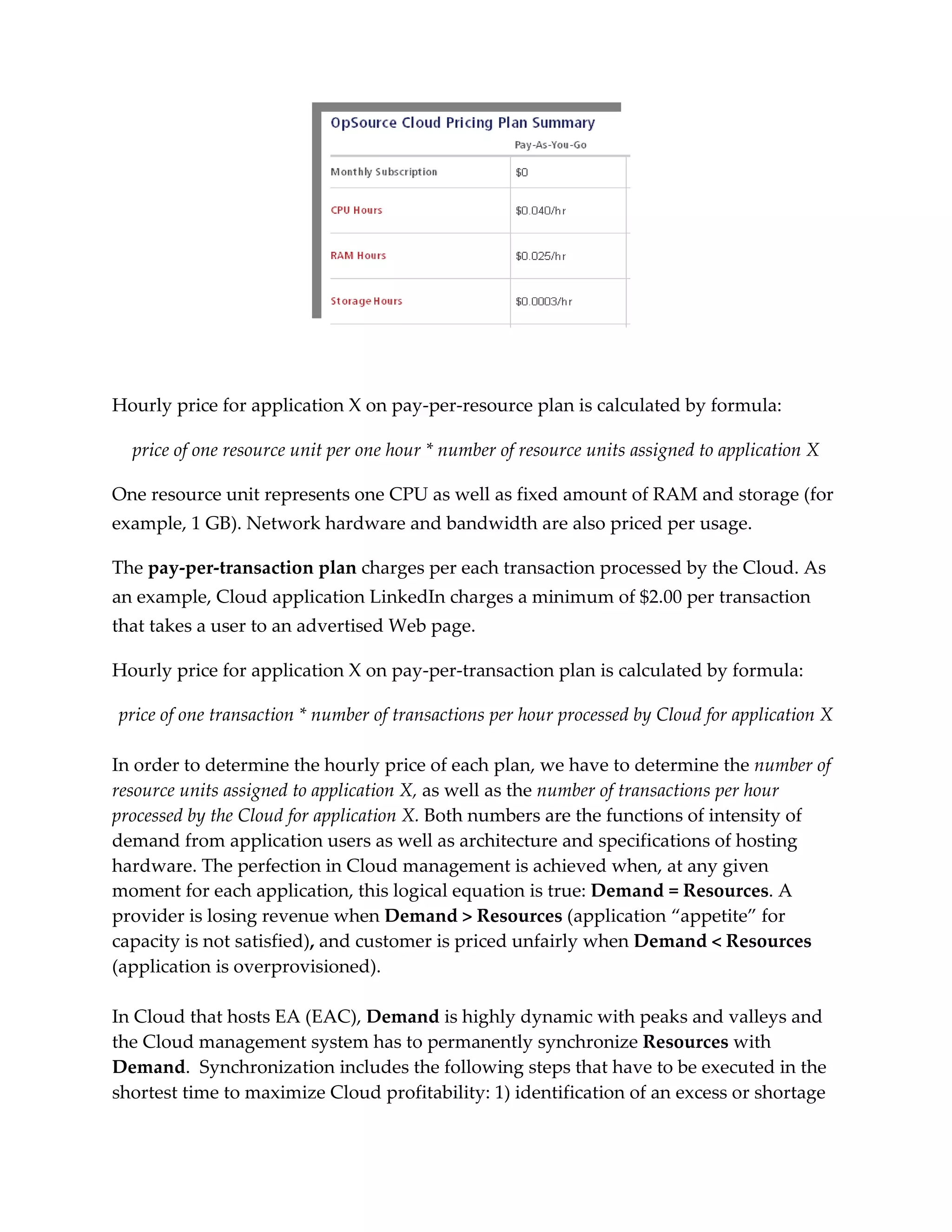
The pay-per-resource plan charges for the hardware capacity an EA uses at any given
time. Typically, resources are priced per hour; below is an excerpt from a price list by
OpSource, a company providing Cloud and managed hosting services:
[http://www.opsource.net/Services/Cloud-Hosting/Pricing]](https://image.slidesharecdn.com/enterpriseapplicationsinthecloud-analysisofpay-per-useplansfinaledited-120729113818-phpapp02/75/Enterprise-applications-in-the-cloud-analysis-of-pay-per-use-plans-1-2048.jpg)
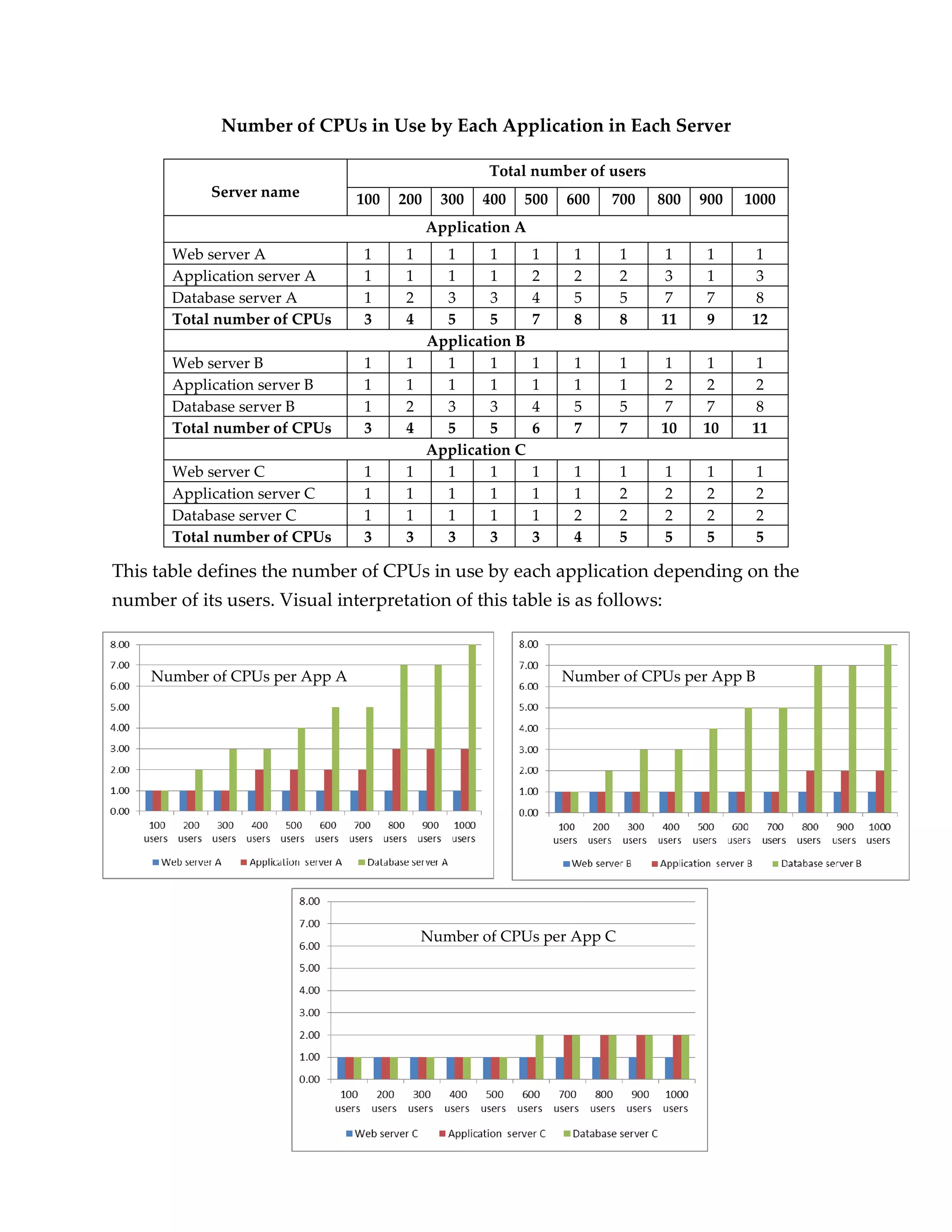

The document discusses the advantages of cloud computing for enterprise applications, focusing on pay-per-use pricing models: pay-per-resource and pay-per-transaction. It highlights the dynamic nature of computing demand and the importance of synchronizing resources with that demand to optimize profitability for cloud providers. The article provides cost/revenue models and insights into how to estimate pricing based on application workloads and resource usage.


![[White Paper] Pay-Per-Applicant, Not Per-Click](https://cdn.slidesharecdn.com/ss_thumbnails/whitepaperpay-per-applicantnotper-click-appcast-150312133701-conversion-gate01-thumbnail.jpg?width=640&height=640&fit=bounds)