This document is the thesis of Eladio Teófilo Ocaña Anaya for the degree of Doctor of University at Université Blaise Pascal in Clermont-Ferrand, France. The thesis is titled "Un schéma de dualité pour les problèmes d'inéquations variationnelles" which translates to "A duality scheme for variational inequality problems". It discusses constructing a general duality scheme for monotone variational inequality problems that is analogous to the classical duality scheme in convex programming by adding perturbation variables. It also studies properties of monotone and maximal monotone multi-valued maps, monotonicity of affine subspaces, and applies the duality
![Introduction
The finite-dimensional variational inequality problem (VIP)
Find x ∈ C such that ∃ x∗ ∈ Γ(¯) with x∗ , x − x ≥ 0 ∀ x ∈ C,
tel-00675318, version 1 - 29 Feb 2012
¯ ¯ x ¯ ¯
−→
where C is a non-empty closed convex subset of R n and Γ : R n −→ R n
a multi-valued map, provides a broad unifying setting of the study of op-
timization and equilibrium problems and serves as the main computational
framework for the practical solution of a host of continuum problems in
mathematical sciences.
The subject of variational inequalities has its origin in the calculus of
variations associated with the minimization of infinite-dimensional functions.
The systematic study of the subject began in the early 1960s with the seminal
work of the Italian mathematician Guido Stampacchia and his collaborators,
who used the variational inequality as an analytic tool for studying free
boundary problems defined by non-linear partial diferential operators arising
from unilateral problems in elasticity and plasticity theory and in mechanics.
Some of the earliest papers on variational inequalities are [16, 21, 22, 40, 41].
In particular, the first theorem of existence and uniqueness of the solution of
VIs was proved in [40].
The development of the finite-dimensional variational inequality and non-
linear inequality problem also began in the early 1960 but followed a different
path. Indeed, the non-linear complementarity problem was first identified in
the 1964 Ph.D. thesis of Richard W. Cottle [8], who studied under the su-
pervision of the eminent George B. Dantzig, “father of linear programming”.
1](https://image.slidesharecdn.com/eladio-120609183205-phpapp02/85/Eladio-7-320.jpg)
![A brief account of the history prior to 1990 can be found in the introduction
in the survey paper [15].
Related to monotone maps, Kachurovskii [17] was apparently the first to
note that the gradients of differentiable convex functions are monotone maps,
and he coined the term “monotonicity” for this property. Really, though, the
theory of monotone mapping began with papers of Minty [25], [26], where
the concept was studied directly in its full scope and the significance of
maximality was brought to light.
His discovery of maximal monotonicity as a powerful tool was one of
the main impulses, however, along with the introduction of sub-gradients
of convex functions, that led to the resurgence of multivalued mapping as
acceptable objects of discourse, especially in variational analysis.
tel-00675318, version 1 - 29 Feb 2012
The need for enlarging the graph of a monotone mapping in order to
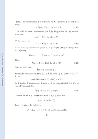
achieve maximal monotonicity, even if this meant that the graph would no
longer be function-like, was clear to him from his previous work with opti-
mization problems in networks, Minty [24], which revolved around the one
dimensional case of this phenomenon; cf. 12.9 [39].
Much of the early research on monotone mapping was centered on infinite
dimensional applications to integral equations and differential equations. The
survey of Kachurovskii [18] and the book of Br´zis [4] present this aspect well.
e
But finite-dimensional applications to numerical optimization has also come
to be widespread particularly in schemes of decomposition, see for example
[7] and references therein.
Duality framework related to variational inequality problems has been
established by many researchers [1],[2],[11],[14],[27],[37],[38]. For example, in
[27] Mosco studied problems of the form
Find x ∈ R n such that 0 ∈ Γ(¯) + ∂g(¯),
¯ x x (1)
where Γ is considered maximal monotone and g a proper lsc convex function
and show that one can always associate a dual problem with (1) defined by
Find u∗ ∈ R n such that 0 ∈ −Γ− (−¯∗ ) + ∂g ∗ (¯∗ ),
¯ u u (2)
where g ∗ denotes the Fenchel conjugate of g.
2](https://image.slidesharecdn.com/eladio-120609183205-phpapp02/85/Eladio-8-320.jpg)
![In this article, he shows that x solves (1) if and only if u∗ ∈ Γ(x) solve
(2).
The above dual formulation and dual terminology is justified by the fact
that this scheme is akin to the Fenchel duality scheme used in convex op-
timization problems. Indeed, if Γ is the subdifferential of some proper lsc
convex function f , the formulations (under appropiate regularity conditions
[35]) (1) and (2) are nothing else but the optimality conditions for the Fenchel
primal-dual pair of convex optimization problems
min{ f (x) + g(x) : x ∈ R n }, min{ f ∗ (−u∗ ) + g ∗ (u∗ ) : u∗ ∈ R n }.
In contrast with this author, Auslender and Teboulle [2] established a dual
framework related to Lagrangian duality (formally equivalent to Mosco’s
tel-00675318, version 1 - 29 Feb 2012
scheme), in order to produce two methods of multipliers with interior multi-
plier updates based on the dual and primal-dual formulations of VIP.
This duality formulation takes its inspiration in the classical Lagrangian
duality framework for constrained optimization problems. In this case the
closed convex subset C is explicitly defined by
C := { x ∈ R n : fi (x) ≤ 0, i = 1, · · · , m },
where fi : R n → R ∪ {+∞}, i = 1, · · · , m, are given proper lsc convex
functions.
In this context, the dual framework established by Auslender and Teboulle
is defined as
∃ x ∈ R n with u∗ ≥ 0 and
¯
Find u∗ ∈ R m such that
¯ 0 ∈ Γ(x) + m u∗ ∂fi (x)
i=1 ¯i (DV P )
0 ∈ −F (x) + NR m (¯∗ ),
+
u
where F (x) = (f1 (x), · · · , fm (x))t . Associated to VIP and DVP, they also
introduce a primal-dual formulation defined by
Find (¯, u∗ ) ∈ R n × R m such that (0, 0) ∈ S(¯, u∗ ),
x ¯ x ¯ (SP )
−→
where S : R n × R m −→ R n × R m is a multivalued map defined by
m
S(x, u∗ ) = { (x∗ , u) : x∗ ∈ Γ(x) + u∗ ∂fi (x), u ∈ −F (x) + NR m (u∗ ) }.
i +
i=1
3](https://image.slidesharecdn.com/eladio-120609183205-phpapp02/85/Eladio-9-320.jpg)
![and
Find u∗ ∈ R m such that ∃ x ∈ R n with ((x, 0), (x∗ , u∗ )) ∈ Φ,
respectively. If Φ is monotone, all the variational problems considered above
are monotone.
As particular examples (Chapter 5) we recover the dual frameworks stud-
ied by Mosco [27] and Auslender and Teboulle [2].
The thesis is divided into 5 chapters:
The first chapter is devoted to set up notations and review some facts
of convex analysis; we describe in details the duality scheme in convex pro-
tel-00675318, version 1 - 29 Feb 2012
gramming. Some facts on multivalued maps are also reviewed.
In Chapter 2, we develop some new general theoretical results on mono-
tone and maximal monotone multi-valued maps (subsets) which will be nee-
ded in our further analysis but are also of interest by themselves. Indeed,
in contrast to the existing literature, new general tools of multi-valued maps
(subsets) are considered in order to characterize and/or study the behaviour
of monotone and maximal monotone from a global and a local point of view.
In this sense, many important results related to monotone and maximal
monotone are recovered as direct consequences of this new approach. In sec-
tion 2.4, we present an algorithm to construct a maximal monotone extension
of an arbitrary monotone map (subset).
Chapter 3, is devoted to the study of monotone and maximal monotone
affine subspaces. Monotonicity and maximal monotonicity of affine subspaces
are explicitly characterized by means of the eigenvalues of bordered matrices
associated to these subspaces. From this characterization, we prove that any
maximal monotone affine subspace can be written (under permutations of
variables) as the graph of an affine map associated to a positive semi-definite
matrix. The algorithm developed in the previous chapter for constructing a
maximal monotone extension is significantly refined. For such subsets, the
maximal monotone affine extension thus constructed is obtained in a finite
number of steps.
5](https://image.slidesharecdn.com/eladio-120609183205-phpapp02/85/Eladio-11-320.jpg)

![the relative boundary, the convex hull, the closure of the convex hull and the
affine hull of a set C, respectively.
The orthogonal subspace to C ⊂ X is defined by
C ⊥ := { y ∈ X : y, x = 0 for all x ∈ C }.
Given a ∈ X, we denote by N (a) the family of neighborhoods of a.
Given a closed set C ⊂ X, we denote by proj C (x) the projection of x onto
C, which is the set of all points in C that are the closest to x for a given
norm, that is
proj C (x) := { y ∈ C : x − y = inf x − y }.
¯ ¯
y∈C
Unless otherwise specified, the norm used is the Euclidean norm. For this
tel-00675318, version 1 - 29 Feb 2012
norm, when C is closed and convex, proj C (x) is reduced to a singleton. In
fact, this property can be used to characterize the closed convex subsets of
X. Indeed C is closed and convex if and only if the projection operator
proj C (·), is single-valued on X [5], [28].
Given a closed convex set C, the normal cone and the tangent cone to C
at x, denoted respectively by NC (x) and TC (x) are defined by
{ x∗ : x∗ , y − x ≤ 0, ∀ y ∈ C } if x ∈ C,
NC (x) :=
∅
if not
and
xk − x
TC (x) = { v : ∃ {xk } ⊂ C, {tk } ⊂ R, xk → x, tk → 0+ and → v }.
tk
We shall use the following convention:
A + ∅ = ∅ + A = ∅, for any set A.
1.2 Convex analysis
Given f : X → (−∞, +∞], we say that f is convex if its epigraph
epi (f) = { (x, α) ∈ X × R : f(x) ≤ α }
8](https://image.slidesharecdn.com/eladio-120609183205-phpapp02/85/Eladio-14-320.jpg)
![is convex in X × R. We say that f is concave if (−f ) is convex. We say that
f is lower semi-continuous (lsc in short) at x if for every λ ∈ R such that
¯
f (¯) > λ there exists a neighborhood V ∈ N (¯) such that x ∈ V , implies
x x
f (x) > λ. f is said to be lsc if it is lsc at every point of X. This is equivalent
to saying that its epigraph is closed in X × R. The function f is said to be
upper semi-continuous (usc in short) if (−f ) is lsc. A convex function f is
said to be proper if f (x) > −∞ for every x ∈ X and its domain
dom (f) = { x ∈ X : f(x) < +∞ }
is nonempty. Note that if f is a convex function, then dom (f) is a convex
set.
Given f : X → (−∞, +∞], its Fenchel-conjugate is
tel-00675318, version 1 - 29 Feb 2012
f ∗ (x∗ ) = sup[ x∗ , x − f (x)],
x∈X
and its biconjugate is
f ∗∗ (x) = sup [ x∗ , x − f ∗ (x∗ )] = sup inf [ x∗ , x − z + f (z)].
x∗ ∈X ∗ x∗ ∈X ∗ z∈X
By construction f ∗ and f ∗∗ are two convex and lsc functions, and f ∗∗ (x) ≤
f (x) for all x ∈ X. A crucial property is the following (see for instance
[3],[10],[35], etc.).
Proposition 1.2.1 Assume that f is a proper convex function on X and lsc
at x. Then f ∗∗ (¯) = f (¯).
¯ x x
Assume that f is a proper convex function and x ∈ X. The subdifferential
of f at x is the set ∂f (x) defined by
∂f (x) = { x∗ ∈ X ∗ : f (x) + x∗ , y − x ≤ f (y), for all y ∈ X }
or equivalently, using the definition of the conjugate,
∂f (x) = { x∗ ∈ X ∗ : f (x) + f ∗ (x∗ ) ≤ x∗ , x }.
Clearly, ∂f (x) = ∅ if x ∈ dom (f) or if f is not lsc at x.
/
9](https://image.slidesharecdn.com/eladio-120609183205-phpapp02/85/Eladio-15-320.jpg)
![By construction, the set ∂f (x) is closed and convex for all x ∈ X. Also
∂f (x) is bounded and nonempty on the interior of dom (f).
The domain of ∂f and its graph are the sets
dom (∂f) = { x ∈ X : ∂f(x) = ∅ },
graph (∂f) = { (x, x∗ ) ∈ X × X∗ : x∗ ∈ ∂f(x) }.
Clearly dom (∂f) ⊂ dom (f) but in general these sets do not coincide, more-
over dom (∂f), unlike dom (f), may be not convex when f is convex as seen
from the following example taken from [35]
Example 1.2.1 Let us define f : R 2 → R by
√
tel-00675318, version 1 - 29 Feb 2012
max{|x1 |, 1 − x2 } if x2 ≥ 0,
f (x1 , x2 ) =
+∞
if not .
It is easily seen that f is convex proper and lsc,
dom (∂f) = (R × [0, +∞[ ) ( ] − 1, +1[×{0})
which is not convex and do not coincide with dom (f).
However it is known that, for a convex function f , the interior (the relative
interior) of dom (∂f) is convex and coincides with the interior (the relative
interior) of dom(f ).
Another very important property of the sub-differential of a convex func-
tion f is the property called cyclic-monotonicity, i.e., for any finite family
{(xi , x∗ ), i = i0 , i1 , · · · , ik+1 } contained in the graph of ∂f such that i0 = ik+1 ,
i
the following inequality holds:
k
x∗i , xji+1 − xji ≤ 0.
j
i=0
In particular, for every x∗ ∈ ∂f (x1 ) and x∗ ∈ ∂f (x2 ), we have
1 2
x∗ − x∗ , x1 − x2 ≥ 0,
1 2
10](https://image.slidesharecdn.com/eladio-120609183205-phpapp02/85/Eladio-16-320.jpg)
![which corresponds to the classical monotonicity of ∂f .
Now, a few words on the continuity properties of the subdifferential. Re-
−→
call that a multivalued map Γ : X −→ X ∗ is said to be closed if its graph
graph (Γ) = { (x, x∗ ) : x∗ ∈ Γ(x) }
is a closed subset of X × X ∗ . The map Γ is said to be usc at x if for all open
¯
subset Ω of X such that Ω ⊃ Γ(¯) there exists a neighborhood V ∈ N (¯)
x x
such that Γ(V ) ⊂ Ω. It is known that the subdifferential of a proper convex
function f is usc at any x ∈ int (dom(f)). Furthermore if in addition f is lsc,
then the map ∂f is closed.
1.3 The duality scheme in convex program-
tel-00675318, version 1 - 29 Feb 2012
ming
Because our duality scheme for monotone variational inequality problems
takes its inspiration in the duality scheme for convex optimization problems,
we describe this scheme in detail.
An optimization problem in X is of the form:
˜
m = min[f (x) : x ∈ C], (PC )
˜
where f : X → (−∞, +∞] and C is a nonempty subset of X. If C is convex
˜
and f is convex, then we are faced with a convex optimization problem.
Step 1. The primal problem :
It consists to replace the constrained problem (PC ) by an equivalent,
apparently unconstrained, problem:
m = min[f (x) : x ∈ X], (P )
˜
with f (x) = f (x) + δC (x), where δC , is the indicator function of C, i.e.,
0 if x ∈ C,
δC (x) =
+∞ if x ∈ C.
/
11](https://image.slidesharecdn.com/eladio-120609183205-phpapp02/85/Eladio-17-320.jpg)
![˜ ˜
If f is convex and C is convex, then f is convex. Also, if f is lsc and C
is closed, then f is lsc. More details on these properties can be found,
for instance, in [3],[10],[35], etc. Of course (PC ) and (P ) have the same
set of optimal solutions. (P ) is called the primal problem.
Step 2. The perturbations :
In this step, we introduce a perturbation function ϕ : X × U →
(−∞, +∞] such that
ϕ(x, 0) = f (x), for all x ∈ X.
Then, we consider the associated perturbed problems
tel-00675318, version 1 - 29 Feb 2012
h(u) = min[ϕ(x, u) : x ∈ X]. (Pu )
The problems (Pu ) are called the primal perturbed problems.
If ϕ is convex on X × U then the problems (Pu ) are convex and the
function h is convex on U . Unfortunately h may be not lsc when ϕ is
lsc.
Denote by S(u) the set of optimal solutions of (Pu ). Then S(0) is
nothing else but the set of optimal solutions of (P ). If ϕ is convex on
X × U , then, for all u ∈ U , S(u) is a convex (may be empty) subset of
X. If ϕ is lsc on X × U , then S(u) is closed.
Step 3. The dual problem :
Let us consider the Fenchel-conjugate function h∗ of h.
h∗ (u∗ ) = sup[ u, u∗ − h(u)]
u
sup[ 0, x + u∗ , u − ϕ(x, u)] = ϕ∗ (0, u∗ ).
x,u
Then, the biconjugate is
h∗∗ (u) = sup[ u∗ , u − ϕ∗ (0, u∗ )].
u∗
12](https://image.slidesharecdn.com/eladio-120609183205-phpapp02/85/Eladio-18-320.jpg)
![By construction, h∗∗ is convex and lsc on U . Furthermore h∗∗ (u) ≤ h(u)
for all u. In particular
md = h∗∗ (0) ≤ h(0) = m.
Let us define the function d : U → [−∞, +∞] by
d(u∗ ) = ϕ∗ (0, u∗ ), ∀ u∗ ∈ U.
Then the dual problem is
−md = −h∗∗ (0) = inf d(u∗ ).
∗
(D)
u
By construction, the function d is convex and lsc. Therefore (D) is a
tel-00675318, version 1 - 29 Feb 2012
convex optimization problem.
There is no duality gap (md = m), if h is a proper convex function
which is lsc at 0.
By analogy with the construction of the primal perturbed problems, we
introduce the dual perturbed problems as
k(x∗ ) = inf ϕ∗ (x∗ , u∗ )
∗
(Dx∗ )
u
and we denote by T (x∗ ) the sets of optimal solutions of these problems.
The function k is convex but not necessarily lsc. The sets T (x∗ ) are
closed and convex but they may be empty. In particular T (0) is the
set of optimal solutions of (D). Furthermore,
k ∗ (x) = ϕ∗∗ (x, 0).
In the particular case where ϕ is a proper lsc convex function on X × U
(this implies that f is convex and lsc on X), ϕ∗∗ = ϕ. It results that
(P ) is the dual of (D) and the duality scheme we have described is
thoroughly symmetric.
Step 4. The Lagrangian function :
13](https://image.slidesharecdn.com/eladio-120609183205-phpapp02/85/Eladio-19-320.jpg)
![Let us define on X × U ∗ the function
L(x, u∗ ) = inf [ −u, u∗ + ϕx (u)]
u
where the function ϕx is defined by
ϕx (u) = ϕ(x, u), for all (x, u) ∈ X × U.
By construction, for any fixed x, the function u∗ → L(x, u∗ ) is concave
and usc because it is an infimum of affine functions. On the other
hand, if ϕ is convex on X × U , then, for any fixed u∗ , the function
x → L(x, u∗ ) is convex on X.
Because the classical sup-inf inequality, we have
tel-00675318, version 1 - 29 Feb 2012
sup inf L(x, u∗ ) ≤ inf sup L(x, u∗ ).
x x
u∗ u∗
Let us compute these two terms.
We begin with the term on the right hand side.
inf sup L(x, u∗ ) = inf sup inf [ 0 − u, u∗ + ϕx (u)] = inf (ϕx )∗∗ (0).
x x u x
u∗ u∗
We know that (ϕx )∗∗ ≤ ϕx . Hence we have the following relation
inf sup L(x, u∗ ) = inf (ϕx )∗∗ (0) ≤ inf ϕx (0) = inf ϕ(x, 0) = m.
x u∗ x x x
Next, we deal with the term on the left.
sup inf L(x, u∗ ) = sup inf [ x, 0 − u, u∗ + ϕx (u)],
u∗ x u∗ (x,u)
= sup[−ϕ (0, u∗ )] = − inf d(u∗ ) = md .
∗
∗
u∗ u
Thus the sup-inf inequality becomes
md = sup inf L(x, u∗ ) ≤ inf sup L(x, u∗ ) = inf (ϕx )∗∗ (0) ≤ m.
x x x
u∗ u∗
Furthermore, if for each x the function ϕx is proper and convex on U
and lsc at 0, then
(ϕx )∗∗ (0) = ϕx (0) = ϕ(x, 0) = f (x).
14](https://image.slidesharecdn.com/eladio-120609183205-phpapp02/85/Eladio-20-320.jpg)
![In this case
inf sup L(x, u∗ ) = inf f (x) = m.
x x
u∗
Step 5. Optimal solutions and saddle points :
By definition, (¯, u∗ ) is said to be a saddle point of L if
x ¯
L(¯, u∗ ) ≤ L(¯, u∗ ) ≤ L(x, u∗ ), for all (x, u∗ ) ∈ X × U ∗ .
x x ¯ ¯
The fundamental property of saddle points is that (¯, u∗ ) is a saddle
x ¯
point of L if and only if
sup inf L(x, u∗ ) = inf sup L(x, u∗ ),
u∗ x x u∗
x is an optimal solution of
¯
tel-00675318, version 1 - 29 Feb 2012
inf [ sup L(x, u∗ ) ]
x u∗
and u∗ is an optimal solution of
¯
sup[ inf L(x, u∗ ) ].
u∗ x
In the case where ϕx is proper convex and lsc on U for all x (this is
true in particular when ϕ proper convex and lsc on X × U ), (¯, u∗ ) is
x ¯
a saddle point of L if and only if m = md (there is no duality gap), x¯
∗
is an optimal solution of (P ) and u is an optimal solution of (D). In
¯
this case, if SP denotes the saddle points set of L, then
SP ⊂ S(0) × T (0).
The equality holds if 0 ∈ ri (proj U (dom (ϕ))).
The following example shows that the previous inclusion can be strict
when 0 ∈ bd (proj U (dom (ϕ))).
Example 1.3.1 Take X = U = R. Define f : X → R ∪ +∞ by
1 if x ≥ 0,
f (x) =
+∞
if not .
15](https://image.slidesharecdn.com/eladio-120609183205-phpapp02/85/Eladio-21-320.jpg)

![tonicity. This condition cannot be translated in terms of graphs. This illus-
trates the fact that monotonicity is a larger concept than convexity.
In order to study the maximal monotonicity of a subset F , it is useful to
introduce the subset F ⊂ X × X ∗ defined by
F = { (x, x∗ ) : x∗ − y ∗ , x − y ≥ 0 for all (y, y ∗ ) ∈ F }.
If G is a monotone subset containing F , then G is contained in F , i.e., F
contains all monotone extensions of F (it results that a subset F is maximal
monotone if and only if F and F coincide). With F is associated the map
−→
Γ : X −→ X ∗ , Γ is maximal monotone if and only if Γ and Γ coincide. The
properties of Γ are studied in section 2.3. Another essential tool introduced
in this subsection in order to study the maximal monotonicity of a monotone
−→
tel-00675318, version 1 - 29 Feb 2012
map Γ is the map ΓS : X −→ X ∗ defined by
graph (ΓS ) = cl [graph (Γ) ∩ (S × X∗ )]
where S is a subset of dom (Γ). A fundamental property is: if V is an open
convex set contained in the convex hull of domain of Γ such that cl (V ∩ S) =
cl (V), then
Γ(x) = co (ΓS (x)) for all x ∈ V.
We shall use this property in section 2.7 to construct a maximal extension
of a monotone map.
−→
In section 2.4, given Γ : X × U −→ X ∗ × U ∗ and a fixed point u ∈ U , we
¯
−→ ∗
study the map Σu : X −→ X defined by
¯
Σu (x) = { x∗ : ∃ u∗ ∈ U ∗ such that (x∗ , u∗ ) ∈ Γ(x, u) }.
¯ ¯
The geometric meaning of this map is that its graph is the projection onto
X × X ∗ of a restriction of the graph of Γ. The introduction of this restriction
is a major tool in the construction of the duality scheme given in chapter 4.
2.1 Definitions and notation
Definition 2.1.1 A set F ⊂ X × X ∗ is said to be monotone if
x∗ − y ∗ , x − y ≥ 0 for all (x, x∗ ), (y, y ∗ ) ∈ F
20](https://image.slidesharecdn.com/eladio-120609183205-phpapp02/85/Eladio-26-320.jpg)
![It is clear that (Γ)− = (Γ− ).
In view of Proposition 2.1.1, the equality Γ = Γ holds if and only if the
multivalued map Γ is maximal monotone. Same fact for Γ− and (Γ− ).
Proposition 2.1.3 Let G ⊂ X × X ∗ . Then, for any x and x∗ the sets Γ(x)
and (Γ− )(x∗ ) are two closed convex sets. In particular, Γ(x) and Γ− (x∗ ) are
closed convex sets when G is maximal monotone.
Proof. By definition,
Γ(x) = { x∗ : x∗ − y ∗ , x − y ≥ 0 }
(y,y ∗ )∈G
and
tel-00675318, version 1 - 29 Feb 2012
Γ− (x∗ ) = { x : x∗ − y ∗ , x − y ≥ 0 }.
(y,y ∗ )∈G
These sets are closed and convex as intersections of half spaces.
Subdifferentials of proper convex lower semi-continuous functions are
maximal monotone maps (see for instance [35]). But a maximal monotone
map is not necessarily associated with a convex function as shown in the
following example.
Example 2.1.1 The map Γ : R 2 → R 2 defined by
x1 −x2
Γ = ,
x2 x1
is maximal monotone. Indeed, by definition,
x∗ x
1 ∈ Γ 1 if and only if
∗
x2 x2
x∗ x1 + x∗ x2 − (x1 + x2 )y1 + (x1 − x∗ )y2 ≥ 0, ∀ (y1 , y2 ) ∈ R 2 ,
1 2
∗
2
which implies that
x∗
1 =
−x2 x1
∗
= Γ .
x2 x1 x2
23](https://image.slidesharecdn.com/eladio-120609183205-phpapp02/85/Eladio-29-320.jpg)

![This is no more true for cyclic monotonicity. To see that, consider the
function ϕ : R × R → (−∞, +∞] defined by
0 if x = u,
ϕ(x, u) =
+∞ if not .
Next, consider for Φ the graph of the subdifferential of ϕ.
Φ = graph (∂ϕ) = { ((x, u), (x∗ , u∗ )) ∈ R 4 : x = u, u∗ = −x∗ }
and
Ψ = { ((x, u∗ ), (x∗ , u)) ∈ R 4 : x = u, u∗ = −x∗ }.
tel-00675318, version 1 - 29 Feb 2012
Φ is maximal cyclically monotone, Ψ is maximal monotone but not cyclically
monotone. Indeed Ψ corresponds to the map Γ defined in example 2.1.1.
However it is easy to see that F ⊂ X × X ∗ is cyclically monotone if and
only if the set F − ⊂ X ∗ × X defined by (x∗ , x) ∈ F − ⇐⇒ (x, x∗ ) ∈ F is
cyclically monotone.
It is very important to know if the monotonicity or maximal monotonicity
holds when we analyze only some projections over appropriate subspaces. In
this sense we present the following proposition.
Proposition 2.2.1 Assume that Φ is a given subset of (X ×U )×(X ∗ ×U ∗ ).
Define E = proj X×X∗ (Φ) and F = proj U×U∗ (Φ). If E and F are (maximal)
monotone, then Φ is (maximal) monotone.
Proof. It is clear that monotonicity of Φ follows from the monotonicity of
E and F . Next, assume that E and F are maximal monotone. In view of
Proposition 2.1.1, it is suffices to show that the inclusion Φ ⊂ Φ is verified.
Let (x, u, x∗ , u∗ ) ∈ Φ. By definition
x∗ − y ∗ , x − y + u∗ − v ∗ , u − v ≥ 0 for all (y, y ∗ ) ∈ E, (v, v ∗ ) ∈ F.
Assume, for contradiction, that (x, x∗ ) ∈ E, then a vector (¯, y ∗ ) ∈ E exists
/ y ¯
∗ ∗ ∗ ∗
so that x − y , x − y < 0 and consequently u − v , u − v > 0, for
¯ ¯
25](https://image.slidesharecdn.com/eladio-120609183205-phpapp02/85/Eladio-31-320.jpg)
![Let some ¯
> 0 be such that < ti for i = 0, 1, · · · , n. Let V be defined by
n n
V = {x = ti xi : 1 = ti and ≤ ti for all i}.
i=0 i=0
Then V is a neighbourhood of x. Given c ∈ R n and x ∈ V , let us define
¯
α(c, x) = sup [ c, x∗ : x∗ ∈ Γ(x) ].
Then,
−∞ ≤ α(c, x) ≤ β(c, x)
where
β(c, x) = sup [ c, x∗ : x∗ , xi − x ≤ x∗ , xi − x , i = 0, 1, 2, · · · , n ].
i (Pe )
x∗
tel-00675318, version 1 - 29 Feb 2012
The dual of the linear program (Pe ) is the problem
n n
β(c, x) = inf [ ui x∗ , xi − x : ui ≥ 0 and
i ui (xi − x) = c ]. (De )
u
i=0 i=0
Because x belongs to V and V is contained in the interior of the convex hull
of the (n + 1) points xi , (De ) is feasible and therefore β(c, x) = β(c, x).
Next, let us consider the linear program
n n
min [ ui : ui ≥ 0 and ui (xi − x) = c ]. (2.1)
i=0 i=0
As (De ), this problem is feasible. We shall show that this problem has one
unique optimal solution that we will denote by u(c, x). Furthermore we shall
prove that the function (c, x) → u(c, x) is continuous on X × V . Indeed, the
n vectors (xi − x), i = 1, 2, · · · , n are linearly independent. Thus, there exist
uniquely defined λi (c, x) ∈ R, i = 1, 2, · · · , n such that
n
c= λi (c, x)(xi − x). (2.2)
i=1
Also, there are uniquely defined γi (c, x) > 0, i = 1, 2, · · · , n such that
n
(x − x0 ) = γi (c, x)(xi − x). (2.3)
i=1
28](https://image.slidesharecdn.com/eladio-120609183205-phpapp02/85/Eladio-34-320.jpg)
![Thus, u is feasible for problem (2.1) if and only if
u ≥ 0 and λi (c, x) = ui − u0 γi (c, x), i = 1, 2, · · · , n (2.4)
and therefore
u0 ≥ 0 and λi (c, x) + u0 γi (c, x) ≥ 0, i = 1, 2, · · · , n.
Problem (2.1) becomes
n
λi (c, x)
inf [ u0 (1 + γi (c, x)) : u0 ≥ max{0, max [ − : i = 1, 2, · · · , n ]} ].
u
0
i=1
i γi (c, x)
n
Since i=1 γi (c, x)) > 0, the previous problem has one unique optimal solu-
tion,
λi (c, x)
tel-00675318, version 1 - 29 Feb 2012
u0 (c, x) = max{0, max [ − : i = 1, 2, · · · , n ]}. (2.5)
i γi (c, x)
Hence problem (2.1) has one unique optimal solution denoted by u(c, x).
In order to prove the continuity of u(c, x), define the n × n matrix
A(x) = [ x1 − x, x2 − x, · · · , xn − x ].
By definition, A(x) is nonsingular for all x ∈ V and the function x → A(x)
is continuous on X. Thus from equations (2.2) and (2.3), the functions
(c, x) → λ(c, x) = [A(x)]−1 c and (c, x) → γ(c, x) = [A(x)]−1 (x − x0 )
are continuous on X × V . Hence, from (2.4) and (2.5), the function (c, x) →
u(c, x) is continuous on X × V .
Next, define
n
ρ(c, x) = ui (c, x) x∗ , xi − x ,
i
i=0
M = sup [ ρ(c, x) : x ∈ V, c ≤ 1 ] and K = {x∗ : x∗ ≤ M }.
x,c
Then for all c such that c ≤ 1 and for all x ∈ V , one has
α(c, x) = sup[ c, x∗ : x∗ ∈ Γ(x) ]
x∗
≤ sup [ c, x∗ : x∗ , xi − x ≤ x∗ , xi − x , i = 0, 1, 2, · · · , n ]
i
x∗
= β(c, x) = β(c, x) ≤ ρ(c, x) ≤ M.
29](https://image.slidesharecdn.com/eladio-120609183205-phpapp02/85/Eladio-35-320.jpg)
![Thus,
sup x∗ ≤ sup [ x∗ : x∗ , xi −x ≤ x∗ , xi −x , i = 0, 1, 2, · · · , n ] ≤ M.
i
x∗ ∈Γ(x) x∗
Then, for all x ∈ V
˜
Γ(x) ⊂ {x∗ : x∗ , xi − x ≤ x∗ , xi − x , i = 0, 1, 2, · · · , n} ⊂ K.
i (2.6)
Therefore the boundedness of Γ on V follows.
Next, we shall prove that Γ(¯) is not empty. Assume, for contradiction,
x
˜ x
that Γ(¯) is empty. Since
˜ x
∅ = Γ(¯) = {¯∗ ∈ R n : x∗ − x∗ , x − x ≥ 0} ⊂ K
x ¯ ¯
(x,x∗ )∈F
tel-00675318, version 1 - 29 Feb 2012
and K is compact, there exist (xj , x∗ ) ∈ F , j = n + 1, n + 2, · · · , n + q such
j
that
∅=( {¯∗ : x∗ − x∗ , x − xj ≥ 0}) ∩ K.
x ¯ j ¯
j=n+1,···,n+q
Next, in view of (2.6),
∅= {¯∗ : x∗ − x∗ , x − xj ≥ 0}.
x ¯ j ¯ (2.7)
j=0,···,n+q
Consider the (n + q + 1) × n matrix A = (¯ − x0 , x − x1 , · · · , x − xn+q ) and
x ¯ ¯
∗
the (n + q + 1) vector a with components aj = xj , x − xj , then (2.7) is
¯
equivalent to
∃ x∗ ∈ R n such that At x∗ ≥ a.
This condition is equivalent to (theorem on alternatives, see for instance [35],
Section 22)
∃ u ∈ R n+q+1 such that u ≥ 0, Au = 0 and a, u > 0.
Without loss of generality, we assume that ui = 1. Then Au = 0 implies
x = ui xi . Next, a, u > 0 implies
¯
n+q n+q n+q
0< uj x ∗ ,
j ui x i − x j = ∗
u i u j x j , xi − x j .
j=0 i=0 i,j
30](https://image.slidesharecdn.com/eladio-120609183205-phpapp02/85/Eladio-36-320.jpg)
![−→
Definition 2.3.1 Let Γ : X −→ X ∗ be a monotone multivalued map and
−→
S ⊂ dom (Γ). We associate with Γ and S the map ΓS : X −→ X ∗ defined
by
graph (ΓS ) = cl [graph (Γ) ∩ (S × X∗ )].
Since Γ is monotone and the closedness of monotone subsets are monotone,
it follows that ΓS is also monotone.
¯ ¯
Next, given x ∈ C = co (dom Γ) and d ∈ TC (¯), we define
x
x ¯ ¯ ¯
γ(¯, d) = lim inf inf [ x∗ , d : x∗ ∈ Γ(¯ + td) ]
∗
x
t→0+ x
and
x ¯ inf [ x∗ , d : x∗ ∈ Γ(¯ + td), x + td ∈ S ].
tel-00675318, version 1 - 29 Feb 2012
γS (¯, d) = lim inf x ¯
(d,t)→(d,0+ ) x∗
¯
Then, we have the following results.
−→
Theorem 2.3.3 Let Γ : X −→ X ∗ be a monotone multivalued map. Denote
D = co (dom (Γ)). Assume that int (D) = ∅ and we are given S ⊂ dom (Γ)
and an open convex subset V of D such that cl (V ∩ S) = cl (V). Then,
a) Γ(x) = co (ΓS (x)), ∀ x ∈ V.
b) Γ is monotone on V .
It follows that any maximal monotone map containing Γ coincides with Γ on
V.
Proof. i) It is clear that graph (ΓS ) ⊂ cl (graph (Γ)) ⊂ graph (Γ). Let x ∈¯
V ⊂ int (D). By Theorem 2.3.1, there exist a compact K and a neighborhood
Vx of x, Vx ⊂ V such that for all x ∈ Vx , ΓS (x) ⊂ Γ(x) ⊂ K. For such x, the
¯ ¯ ¯ ¯
set ΓS (x) is bounded, it is closed since graph (ΓS ) is closed. Therefore, one
has
co (ΓS (x)) = co (ΓS (x)) ⊂ Γ(x), ∀ x ∈ Vx .
¯
ii) Next, we prove that Γ(¯) ⊂ co (ΓS (¯)). Assume, for contradiction,
x x
∗ ∗
that there exists a ∈ Γ(¯) such that a ∈ co (ΓS (¯)). In view of separation
x / x
34](https://image.slidesharecdn.com/eladio-120609183205-phpapp02/85/Eladio-40-320.jpg)
![theorems (see for instance [35], section 11), there exists a vector d, d = 1,
such that
sup[ d, ξ ∗ − a∗ : ξ ∗ ∈ co (ΓS (¯)) ] < 0.
x (2.9)
Since cl (V ∩ S) = cl (V), there exist a sequence of vectors {dk } ∈ X and a
sequence of positive real numbers {tk } such that
xk = x + tk dk ∈ S ∩ Vx , dk → d and tk → 0 as k → +∞.
¯ ¯
Let x∗ ∈ Γ(xk ), then x∗ ∈ K. Without loss of generality, we assume that the
k k
whole sequence {x∗ } converges to some x∗ . Then x∗ ∈ ΓS (¯).
k ¯ ¯ x
On the other hand, since
a∗ ∈ Γ(¯) = { x∗ : x∗ − x∗ , x − x ≥ 0, ∀(x, x∗ ) ∈ graph (Γ) }
tel-00675318, version 1 - 29 Feb 2012
x ¯ ¯ ¯
and for all k, (xk , x∗ ) ∈ graph (Γ), then
k
1 ∗
x∗ − a∗ , dk =
k x − a∗ , xk − x ≥ 0.
¯
tk k
Thus, for every k
x∗ − a∗ , dk ≥ 0.
k
Passing to the limit, we obtain x∗ − a∗ , d ≥ 0, in contradiction with (2.9).
¯
iii) It remains to prove that Γ is monotone on V . It suffices to show that
ΓS is monotone on V . Let x∗ ∈ ΓS (x) and y ∗ ∈ ΓS (y). Then, there exist
two sequences {(xk , x∗ )} and {(yk , yk )} in graph (Γ) that converge to (x, x∗ )
k
∗
and (y, y ∗ ) respectively. Since Γ is monotone, one has x∗ − yk , xk − yk ≥ 0.
k
∗
Passing to the limit, we obtain
x∗ − y ∗ , x − y ≥ 0
as required.
−→
Corollary 2.3.2 Let Γ : X −→ X ∗ be a monotone multivalued map and
x ∈ int (dom(Γ)). Assume that Γ(¯) is a convex subset of X ∗ and the map Γ
¯ x
is closed on a neighborhood W of x. Then Γ(¯) = Γ(¯).
¯ x x
35](https://image.slidesharecdn.com/eladio-120609183205-phpapp02/85/Eladio-41-320.jpg)
![Proof. Choose for W a convex open neighborhood, next set S = W in
the theorem. The closedness of Γ implies that ΓS (¯) = Γ(¯), and therefore
x x
Γ(¯) = Γ(¯) as required.
x x
Theorem 2.3.4 Under the assumptions of Theorem 2.3.3, it holds, for all
¯
x ∈ V and d ∈ X:
¯
a) x ¯
γ(¯, d) = ¯ ¯
lim inf [ x∗ , d : x∗ ∈ Γ(¯ + td) ].
x
t→0+ x∗
b) x ¯
γ(¯, d) = ¯ ¯
lim sup [ x∗ , d : x∗ ∈ Γ(¯ + td) ].
x
t→0+ x∗
c) x ¯ ∗¯
γ(¯, d) = sup [ x , d : x∗ ∈ Γ(¯) ].
x
d) x ¯ x ¯
γ(¯, d) = γS (¯, d).
tel-00675318, version 1 - 29 Feb 2012
Proof.
¯ ¯ ¯
a,b) Let t1 , t2 be such that 0 < t1 < t2 and x + t1 d, x + t2 d ∈ V . Since Γ is
¯
¯ ∗
monotone on V , for all x∗ ∈ Γ(¯ + t1 d), x2 ∈ Γ(¯ + t2 d),
x x ¯
1
¯
(t2 − t1 ) x∗ − x∗ , d ≥ 0
2 1
and therefore
¯ ¯ ¯
x∗ , d ≥ x∗ , d , ∀ x∗ ∈ Γ(¯ + ti d), i = 1, 2.
x
2 1 i
It follows that
¯ ¯ ¯ ¯
sup[ x∗ , d : x∗ ∈ Γ(¯ + t2 d) ] ≥ inf[ x∗ , d : x2 ∈ Γ(¯ + t2 d) ] ≥
x ∗
x
2 2 2
¯ x ¯ ¯ x ¯
≥ sup[ x∗ , d : x∗ ∈ Γ(¯ + t1 d) ] ≥ inf[ x∗ , d : x∗ ∈ Γ(¯ + t1 d) ].
1 1 1 1
Hence
x ¯
γ(¯, d) = ¯ ¯
lim inf [ x∗ , d : x∗ ∈ Γ(¯ + td) ]
x
t→0+ x∗
= ¯ ¯
lim sup [ x∗ , d : x∗ ∈ Γ(¯ + td) ].
x
t→0+ x∗
36](https://image.slidesharecdn.com/eladio-120609183205-phpapp02/85/Eladio-42-320.jpg)
![¯ ¯
c) For any t > 0 such that x + td ∈ V and x∗ ∈ Γ(¯ + td) one has
¯ x
t
¯ 1 ¯ ¯
x∗ − x∗ , d = x∗ − x∗ , x + td − x ≥ 0 for all x∗ ∈ Γ(¯),
t ¯ x
t t
and therefore
x ¯ ¯
γ(¯, d) ≥ sup [ x∗ , d : x∗ ∈ Γ(¯) ].
x
Now suppose, for contradiction, that the converse inequality does not
hold. Then there exists λ such that
x ¯ ¯
γ(¯, d) > λ > sup [ x∗ , d : x∗ ∈ Γ(¯) ].
x
¯ ¯ ¯ ¯
Since Γ is usc in x, there exists t > 0 such that for all t ∈]0, t[, x +td ∈ V
¯
and
tel-00675318, version 1 - 29 Feb 2012
¯ ¯
λ > sup [ x∗ , d : x∗ ∈ Γ(¯ + td) ].
x
x∗
Then
¯ ¯ x ¯
λ ≥ lim inf sup [ x∗ , d : x∗ ∈ Γ(¯ + td) ] ≥ γ(¯, d).
x
t→0+ x∗
In contradiction with the assumption on λ.
d) We shall prove that
x ¯
γ(¯, d) = lim inf inf [ x∗ , d : x∗ ∈ Γ(¯ + td), x + td ∈ x∗ ∈ S ]
x ¯ ¯
(d,t)→(d,0+ ) x∗
¯
= lim sup sup [ x∗ , d : x∗ ∈ Γ(¯ + td), x + td ∈ S ],
x ¯
(d,t)→(d,0+ ) x∗
¯
from what the result will follow. By definition, for all t > 0
1 ∗
x∗ − x∗ , d =
¯ x − x∗ , (¯ + td) − x ≥ 0 ∀x∗ ∈ Γ(¯ + td), x∗ ∈ Γ(¯).
¯ x ¯ x ¯ x
t
Then
inf [ x∗ , d : x∗ ∈ Γ(¯ + td), x + td ∈ S ] ≥ x∗ , d
∗
x ¯ ¯ for all x∗ ∈ Γ(¯),
¯ x
x
and therefore, for all x∗ ∈ Γ(¯),
¯ x
∗
x ¯ ¯ ¯
lim inf inf [ x∗ , d : x∗ ∈ Γ(¯ + td), x + td ∈ S ] ≥ x∗ , d .
¯
(d,t)→(d,0+ ) x
37](https://image.slidesharecdn.com/eladio-120609183205-phpapp02/85/Eladio-43-320.jpg)
![Then, it follows from c),
x ¯ x ¯
lim inf inf [ x∗ , d : x∗ ∈ Γ(¯ + td), x + td ∈ S ] ≥ γ(¯, d). (2.10)
(d,t)→(d,0+ ) x∗
¯
On the other hand, since Γ is usc in x, given > 0, there exist δ > 0
¯
¯
and an open bounded convex neighborhood Wd of d, such that t ∈ (0, δ)
¯
and d ∈ Wd , implies x + td ∈ V and
¯ ¯
Γ(¯ + td) ⊂ Γ(¯) + B1 (0), ∀ x + td ∈ V ∩ S ,
x x ¯
where B1 (0) is the Euclidean unit ball of X ∗ . It follows from c),
x ¯ x ¯
lim sup sup [ x∗ , d : x∗ ∈ Γ(¯ + td), x + td ∈ S ] ≤ γ(¯, d) + M,
(d,t)→(d,0+ ) x∗
¯
tel-00675318, version 1 - 29 Feb 2012
for some M > 0. Taking → 0+ ,
t t ¯ x ¯
lim sup sup [ x∗ , d : x∗ ∈ Γ(¯ + td), x + td ∈ S ] ≤ γ(¯, d). (2.11)
x
¯
(d,t)→(d,0+ )
The result follow from (2.10) and (2.11).
The two latter results were concerned with points in the interior of C =
co (dom Γ). Next, we consider points belonging to the boundary of C. We
begin with the following proposition.
−→
Proposition 2.3.3 Let Γ : X −→ X ∗ be a monotone multivalued map.
Assume that int (C) = ∅, x ∈ bd (C) and there exist a subset S ⊂ dom (Γ)
¯
and a neighborhood V of x satisfying cl (V ∩ S) = cl (V ∩ C).
¯
Assume also that there exists a sequence {(xk , x∗ )}k∈IN ⊂ (S × X∗ ) ∩
k
¯ ¯
graph (Γ) such that xk = x + tk dk , tk → 0+ , dk → d ∈ int (TC (¯)) and
x
∗
xk → +∞. Then,
a) ΓS (¯) = Γ(¯) = ∅,
x x
b) γS (¯, d) = γ(¯, d) = −∞, ∀ d ∈ int (TC (¯)),
x x x
c) For all (xk , x∗ ) ∈ graph (Γ) with {xk } converging to x one has x∗ →
k ¯ k
+∞.
38](https://image.slidesharecdn.com/eladio-120609183205-phpapp02/85/Eladio-44-320.jpg)
![c) Follows from a) and from the fact that graph (Γ) is closed.
The following result establishes a formulation of Γ on the boundary of
the convex hull of dom (Γ).
−→
Theorem 2.3.5 Let Γ : X −→ X ∗ be a monotone multivalued map. Denote
by C the closure of the convex hull of dom (Γ). Assume that int (C) = ∅, that
x ∈ bd (C) and that there exist a subset S ⊂ dom (Γ) and a neighborhood
¯
V ∈ N (¯) satisfying cl (V ∩ S) = cl (V ∩ C). Then,
x
Γ(¯) = co (ΓS (¯))) + NC (¯).
x x x
Proof. i) We prove that co (ΓS (¯)) + NC (¯) ⊂ Γ(¯). Indeed, by definition,
x x x
tel-00675318, version 1 - 29 Feb 2012
graph (ΓS ) ⊂ cl (graph (Γ)) ⊂ graph (Γ).
Thus, ΓS (¯) ⊂ Γ(¯) and therefore co (ΓS (¯)) ⊂ Γ(¯) because Γ(¯) is closed
x x x x x
and convex. On the other hand, by Proposition 2.3.2, Γ(¯) = Γ(¯) + NC (¯).
x x x
It follows that
co (ΓS (¯)) + NC (¯) ⊂ Γ(¯).
x x x
ii) We prove that co (ΓS (¯)) + NC (¯) is closed. In view of the result on
x x
the closure of the sum of two closed convex sets, it is enough to prove that
−NC (¯) ∩ [co (ΓS (¯))]∞ = {0}.
x x
Since co (ΓS (¯)) ⊂ Γ(¯), Proposition 2.3.2 implies
x x
[co (ΓS (¯))]∞ ⊂ (Γ(¯))∞ ⊂ NC (¯).
x x x
Next, − NC (¯) ∩ NC (¯) = {0}, because int (C) = ∅. Therefore,
x x
−NC (¯) ∩ [co (ΓS (¯))]∞ ⊂ −NC (¯) ∩ NC (¯) = {0},
x x x x
as required.
iii) We prove that Γ(¯) ⊂ co (ΓS (¯)) + NC (¯). Assume, for contradic-
x x x
∗ ∗
tion, that there exists x ∈ Γ(¯) such that x ∈ co (ΓS (¯)) + NC (¯). Since
¯ x ¯ / x x
40](https://image.slidesharecdn.com/eladio-120609183205-phpapp02/85/Eladio-46-320.jpg)
![co (ΓS (¯)) + NC (¯) is closed and convex, applying separation theorems (see
x x
¯ ¯
for instance [35], section 11), there exists a vector d, d = 1 such that
¯ x ∗
x ¯¯
sup[ d, x∗ + x∗ : x∗ ∈ ΓS (¯), x2 ∈ NC (¯) ] < d, x∗ . (2.13)
1 2 1
Since NC (¯) is a cone,
x
¯
0 = sup [ d, x∗ : x∗ ∈ NC (¯) ].
x (2.14)
2 2
¯
Hence d ∈ TC (¯). On the other hand, combining (2.14) and (2.13) one
x
obtains
¯
sup [ d, x∗ − x∗ : x1 ∈ ΓS (¯) ] < 0.
¯ ∗
x
We shall show that there exists some d ∈ int (TC (¯)) such that
x
tel-00675318, version 1 - 29 Feb 2012
sup [ d, x∗ − x∗ : x∗ ∈ ΓS (¯) ] < 0.
¯ 2 x
Take some v ∈ int (TC (¯)). For all positive integer k, set
x
¯ 1
dk = d + v ∈ int (TC (¯)).
x
k
We shall prove that for k large enough
sup [ dk , x∗ − x∗ : x∗ ∈ ΓS (¯) ] < 0.
¯ x
If not, for all k, there exists x∗ ∈ ΓS (¯) such that
k x
1 ¯
+ dk , x∗ − x∗ ≥ 0 > d, x∗ − x∗ .
k ¯ k ¯ (2.15)
k
Since ΓS (¯) is closed, it follows that x∗ → +∞ as k → +∞. Without loss
x k
x∗
of generality, we assume that x∗ converges to w∗ . Then, proceeding as in
k
k
the proof Proposition 2.3.3 a), w∗ ∈ NC (¯). The relations in (2.15) imply
x
1 x∗
k x∗
¯ 1 1 1 x∗
k x∗
¯
∗
+ v, ∗ − ∗ = k[ ∗
+ v, ∗ − ∗ ] > 0.
xk xk xk k xk k xk xk
Passing to the limit,
v, w∗ ≥ 0,
41](https://image.slidesharecdn.com/eladio-120609183205-phpapp02/85/Eladio-47-320.jpg)
![a contradiction. Hence there exists d ∈ int (TC (¯)) such that
x
sup [ d, x∗ : x∗ ∈ ΓS (¯) ] < d, x∗ .
2 2 x ¯ (2.16)
Next, let us consider a sequence {(xk , x∗ )} ⊂ (S × X∗ ) ∩ graph (Γ) such
k
that xk = x + tk dk , tk → 0+ , dk → d. Since d ∈ int (TC (¯)) and, by
¯ x
assumption, Γ(¯) is not empty, Proposition 2.3.3 implies that the sequence
x
{x∗ } is bounded. Without loss of generality it can be assumed that x∗
k k
∗ ∗
converges to some x . Then x ∈ ΓS (¯).
x
∗
On the other hand, since x ∈ Γ(¯),
¯ x
1 ∗
x∗ − x∗ , dk =
¯ k x − x∗ , xk − x ≤ 0, ∀ k ∈ IN.
¯ k ¯
tk
tel-00675318, version 1 - 29 Feb 2012
Passing to the limit
x∗ − x∗ , d ≤ 0,
¯ with x∗ ∈ ΓS (¯),
x
a contradiction with (2.16). Hence
Γ(¯) ⊂ co (ΓS (¯)) + NC (¯),
x x x
as required.
We summarize the different results above in the following theorem.
−→
Theorem 2.3.6 Let Γ : X −→ X ∗ be a monotone multivalued map. Denote
by C the closure of the convex hull of dom (Γ). Assume that int (C) = ∅ and
that there exists S ⊂ dom (Γ) such that cl (S) = C. Then, the multivalued
−→
map Λ : X −→ X ∗ defined by
co (ΓS (x)) + NC (x)
if x ∈ C,
Λ(x) =
∅ if x ∈ C,
/
is the unique maximal monotone map containing Γ with domain contained
in C.
42](https://image.slidesharecdn.com/eladio-120609183205-phpapp02/85/Eladio-48-320.jpg)
![Hence, the maximality of Λ1 , implies that
Λ1 (x) = Λ1 (x) + NC (x) = Γ(x) + NC (x) = Λ(x) for all x ∈ X
and the uniqueness follows.
Remark. The above theorem is an extension of the well known result
on convex functions (see for instance [35]): assume that f is proper, convex,
lower semicontinuous and such that int (dom (f)) = ∅. Then
∂f (x) = co (S(x)) + K(x) for all x,
where K(x) is the normal cone to dom (f) at x (empty if x ∈ dom (f)) and
/
S(x) is the set of all limits of sequences of the form { f (xk )} such that f
tel-00675318, version 1 - 29 Feb 2012
is differentiable at xk and {xk } tends to x. We will see later, that maximal
monotone maps are reduced to a point almost everywhere on the interior of
their domain.
As a direct consequence of this theorem we have the well known result
on the sum of two maximal monotone maps.
−→
Proposition 2.3.4 Let Γi : X −→ X ∗ , i = 1, 2, be two maximal monotone
maps. Assume that int (dom (Γ1 ))∩int (dom (Γ2 )) = ∅. Then the multivalued
−→
map Γ : X −→ X ∗ defined by
Γ(x) = Γ1 (x) + Γ2 (x)
is also maximal monotone.
Proof. Denote by C the closure of dom (Γ) = dom (Γ1 ) ∩ dom (Γ2 ). It is
clear C is convex with nonempty interior. Consider S ⊂ int (C) such that
cl (S) = C. In view of Theorem 2.3.6, we shall prove that
co (ΓS (x)) + NC (x) ⊂ Γ(x) for all x ∈ X.
∗
We first prove that Γ is closed. Let {(xk , xk )} ⊂ graph (Γ) such that
(xk , x∗ ) → (x, x∗ ). Then there exist two sequences {x∗ } and {x∗ } with
k 1k 2k
x∗ ∈ Γ1 (xk ), x∗ ∈ Γ2 (xk ) and x∗ + x∗ = x∗ .
1k 2k 1k 2k
45](https://image.slidesharecdn.com/eladio-120609183205-phpapp02/85/Eladio-51-320.jpg)

![(x, 0) ∈ int (K). Then 0 ∈ bd (C) and the following relation holds between
the normal cones at (0, 0) ∈ K and 0 to C
x∗ ∈ NC (0) ⇐⇒ ∃ u∗ ∈ R p such that (x∗ , u∗ ) ∈ NK (0, 0).
Proof. It is clear that if (x∗ , u∗ ) ∈ NK (0, 0) then x∗ ∈ NC (0). To show
the converse statement, assume that x∗ ∈ NC (0), x∗ = 0. Then, because
0 ∈ bd (C),
0 = inf [ −x∗ , x : x ∈ C ].
x
(P )
Let us consider a convex function g : R n × R p →] − ∞, +∞[ such that
g(x, 0) < 0, K = { (x, u) : g(x, u) ≤ 0 } ⊂ int (dom (g)).
tel-00675318, version 1 - 29 Feb 2012
Such a function is easily constructed. Then (P) can be written as
0 = inf [ −x∗ , x + 0, u : g(x, u) ≤ 0, u = 0 ]. (P )
x,u
Because the Slater condition holds for this convex problem and (0, 0) is so-
lution, there is λ ≥ 0, (z ∗ , v ∗ ) ∈ ∂g(0, 0) and w∗ ∈ R p such that
−x∗ + λz ∗ = 0, λv ∗ + w∗ = 0.
Then, because x∗ = 0, λ > 0 and λ−1 (x∗ , −w∗ ) ∈ NK (0, 0). It follows that
(x∗ , −w∗ ) ∈ NK (0, 0).
Now, we can prove the following basic result.
−→
Theorem 2.4.2 Assume that Γ : X × U −→ X ∗ × U ∗ is maximal monotone
and the interior of its domain is nonempty. Let u ∈ proj U (int (dom (Γ))).
¯
Then, Σu is maximal monotone on X.
¯
Proof. i) Let x ∈ int (dom(Σu )), then (x, u) ∈ int (dom (Γ)). Theorem 2.4.1
¯ ¯
implies that Σu (x) = Σu (x). We have proved that Σu is maximal monotone
¯ ¯ ¯
on the interior of its domain.
ii) Next, consider some x in the boundary of the domain of Σu . Proceeding
¯
as in Theorem 2.4.1 we see that Σu (x) is convex. We shall prove that Σu
¯ ¯
∗
is closed in x. Consider any sequence {(xk , xk )} ⊂ graph (Σu ) converging
¯
48](https://image.slidesharecdn.com/eladio-120609183205-phpapp02/85/Eladio-54-320.jpg)
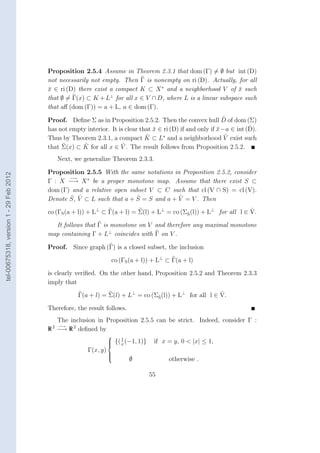
![Finally, the following proposition is an extension of Theorem 2.4.2.
−→
Proposition 2.5.7 Assume that Γ : X × U −→ X ∗ × U ∗ is maximal mono-
−→
tone and u ∈ proj U (ri (dom (Γ))). Then the multivalued map Σu : X −→ X ∗
¯ ¯
defined by
Σu (x) = { x∗ : ∃ u∗ ∈ U ∗ such that (x∗ , u∗ ) ∈ Γ(x, u) }
¯ ¯
is maximal monotone.
It follows that the relative interior and the closure of dom (Σu ) are convex
¯
and satisfy the following relations
cl (ri (dom (Σu ))) = cl (dom (Σu ))
¯ ¯ and ri (cl (dom (Σu ))) = ri (dom (Σu )).
¯ ¯
Furthermore,
tel-00675318, version 1 - 29 Feb 2012
x ∈ rbd (dom (Σu )) ⇐⇒ (x, u) ∈ rbd (dom (Γ)).
¯ ¯
Proof. In order to simplify the notations, assume, without loss of generality,
that (0, 0) ∈ ri (dom (Γ)) and u = 0.
¯
The linear subspace L = aff (dom (Γ)) can be written as
L = { (x, u) ∈ X × U : Ax + Bu = 0 },
where A and B are two matrices of appropriate order. Then
L⊥ = img ([A, B]t )
and aff (dom (Σ0 )) = ker(A).
−→
Define Σ : L −→ L∗ = L by
Γ(x, u) = Σ(x, u) + L⊥ ,
then Σ is maximal monotone, by Proposition 2.5.1 b). This implies that the
−→
multivalued map Σ0 : ker(A) −→ ker(A) defined by
Σ0 (x) = { x∗ : ∃ u∗ ∈ proj U∗ (L∗ ) such that (x∗ , u∗ ) ∈ Σ(x, 0) }
is also maximal monotone.
By definition,
Σ0 = Σ0 + img (At ) = Σ0 + (ker(A))⊥ ,
from what we deduce that Σ0 is maximal monotone.
57](https://image.slidesharecdn.com/eladio-120609183205-phpapp02/85/Eladio-63-320.jpg)
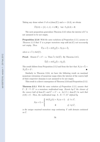
![Proof. Define the set
A = { x ∈ dom (Γ) : ∃ x∗ ∈ Γ(x), x∗ , x − x ≤ 0 }.
ˆ
Clearly, A is bounded and Γ− (0) ⊂ A. Consider r > 0 such that the Eu-
−→
clidean ball Br (ˆ) contains A. Define F : X −→ X ∗ by F (x) = Γ(x) +
x
NB2r (ˆ) (x). Since x ∈ ri (dom (Γ)) ∩ B2r (ˆ), F is maximal monotone and
x ˆ x
therefore, since dom (F) is bounded, there exists x ∈ B2r (ˆ) such that
¯ x
0 ∈ F (¯) = Γ(¯) + NB2r (ˆ) (¯).
x x x x
Let x∗ ∈ NB (¯) such that −¯∗ ∈ Γ(¯). Let us prove that x ∈ A. For that,
¯ x x x ¯
assume, for contradiction, that x ∈ A. Since x ∈ NB (¯), x∗ , x − x ≥ 0, for
¯/ ¯ ∗
x ¯ ¯
tel-00675318, version 1 - 29 Feb 2012
∗
all x ∈ B. In particular, for x = x, we have x , x − x ≥ 0. On the other
ˆ ¯ ¯ ˆ
∗ ∗
hand, since x ∈ A and −¯ ∈ Γ(¯), x , x − x < 0, which is not possible.
¯ / x x ¯ ¯ ˆ
∗
Hence x ∈ A, and therefore x = 0. Thus, 0 ∈ Γ(¯), as required.
¯ ¯ x
−→
Theorem 2.6.1 Let Γ : X −→ X ∗ be a maximal monotone multivalued map
such that C = int (dom(Γ)) = ∅. Then Γ is single-valued almost everywhere
(in the Lebesgue sense) on C.
Proof. The result, when dim(X) = 1, is a well known result on monotonic
functions of one real variable, see for instance Natanson [29]. Assume that
dim(X) = n > 1. For every i = 1, · · · , n, let us define, for every x ∈ C,
θi (x) = max [ x∗ − y ∗ , ei : x∗ , y ∗ ∈ Γ(x) ],
where for i = 1, · · · , n, ei denotes the ith canonical vector in X. Since Γ(x)
is compact for all x ∈ C and the map Γ is usc, the function θi is upper
semicontinuous and therefore measurable on C. Thus the set Di = {x ∈ C :
θi (x) ≤ 0} is measurable because C is convex and open.
Let x ∈ D = ∩i=1 Di . If x∗ , y ∗ ∈ Γ(x), then |x∗ − yi | ≤ 0 for all i. Hence
n
i
∗
x∗ = y ∗ . Thus D is the set of x ∈ C such that Γ(x) is reduced to a singleton.
D and their complement Dc = ∪n Di are measurable. We shall prove that
i=1
c
for all i, meas (Dc ) = 0, from what it is deduced that meas (Dc ) = 0. We give
i
62](https://image.slidesharecdn.com/eladio-120609183205-phpapp02/85/Eladio-68-320.jpg)
![the proof for i = n. In fact, we shall prove that meas (Dc ∩ P) = 0, for all
P of the type P = n [¯i , xi + ], with > 0, from what the result follows.
i=1 x ¯
c
Denotes by 1Dn the characteristic function of Dn defined by
c
c
1 if x ∈ Dn ,
1Dn (x) =
c
0 / c
if x ∈ Dn .
By Fubini’s theorem,
xn +
¯
meas (Dc ∩ P) =
n 1Dc (x)dx =
n
[ 1Dc (x)dxn ]dx1 · · · dxn−1 ,
n
(2.26)
P Q xn
¯
where Q = {y = (x1 , · · · , xn−1 ) ∈ R n−1 : ∃ xn with (x1 , · · · , xn−1 , xn ) ∈ P ∩
C}. For y ∈ Q, let us define
D(y) = {xn ∈ R : (y, xn ) ∈ Dn ∩ P }.
tel-00675318, version 1 - 29 Feb 2012
−→
By definition, D(y) is the set of points where the multivalued map hy : R −→
R defined by
hy (t) = Γ(y, xn + t), en
¯
is reduced to a singleton. This map hy is monotone. Applying again the result
on monotonic functions of one real variable, we obtain that meas ([D(y)]c ) =
0. Report in (2.26), we deduce that meas (Dc ∩ P) = 0.
n
2.7 Maximal monotone extensions
¯
Let G be a subset of X × X ∗ . If G is not monotone, there is no G monotone
containing G. If G is monotone, with an argument based on the axiom of
choice, it is possible to prove that there exists a maximal monotone extension
of G. This extension is not unique as seen in the following example:
Example 2.7.1 G = {(−1, −1), (1, 1)} ⊂ R 2 , G is monotone. The two
following sets
G1 = {(x, x∗ ) ∈ R 2 : x∗ = x} ,
G2 = ] − ∞, 1] × {−1} ∪ {1} × [−1, ∞[
are maximal monotone, and they both contain G.
63](https://image.slidesharecdn.com/eladio-120609183205-phpapp02/85/Eladio-69-320.jpg)
![The axiom of choice is not constructive. We shall show how to construct a
maximal monotone extension.
−→
Let F : X −→ X ∗ be a monotone map. Denote by C, the closure of
the convex hull of dom (F). We assume that int (C) is nonempty and we are
given a countable set S = {x0 , x1 , · · · , xn , · · ·} ⊂ int (C) such that cl (S) = C.
In the construction, by convention, A + ∅ = ∅.
Algorithm:
−→
Step 0 Define F0 : X −→ X ∗ by
F (x) + NC (x)
if x ∈ C,
F0 (x) =
∅
if not .
tel-00675318, version 1 - 29 Feb 2012
By construction F0 is monotone and dom (F0 ) = dom (F).
Step k In the previous steps a monotone map Fk has been obtained with
graph (Fk ) ⊃ graph (F).
• If dom (Fk ) ⊃ S, by Theorem 2.3.6, the multivalued map
−→
x −→ Fk (x) + NC (x)
is maximal monotone. STOP.
• If not, take
p(k) = min[ p ∈ IN : xp ∈ S ∩ (dom (Fk ))c ],
and define
Fk (x) if x ∈ dom (Fk ),
Fk+1 (x) = Fk (xp(k) ) if x = xp(k) ,
∅ otherwise .
By construction, Fk+1 is monotone,
graph (F) ⊂ graph (Fk ) ⊂ graph (Fk+1 )
64](https://image.slidesharecdn.com/eladio-120609183205-phpapp02/85/Eladio-70-320.jpg)


![It is clear that any affine subspace of R n × R n can be written in this way.
In sections 3.1 and 3.2 we characterize the monotonicity and the maximal
monotonicity of these subspaces. An important result shows that at any
maximal monotone subset is associated a permutation of the variables and a
positive subdefinite matrix. Based on this result, we give a finite algorithm
to obtain a maximal monotone affine extension of a monotone map subspace.
The linearity structure allows a quite simpler construction than the one given
in Chapter 2 for non affine subspaces.
The last section is concerned with the restriction of an affine monotone
subspace.
3.1 Monotone affine subspaces
tel-00675318, version 1 - 29 Feb 2012
In this section we consider subsets of R n × R n of the form
E = { (x, x∗ ) ∈ R n × R n : Ax + Bx∗ = c },
where c ∈ R p , A and B are two p × n matrices.
Without loss of generality, we assume that there is no redundance in the
linear system, i.e., the p × 2n matrix C = [A, B] is of rank p.
By definition, the set E is monotone if and only if
inf[ x2 − x∗ , x2 − x1 : (xi , x∗ ) ∈ E, i = 1, 2 ] ≥ 0.
∗
1 i
Denote P the 2n × 2n matrix defined by
0 I
P = ,
I 0
where I is the identity matrix of order n; then the monotonicity of E is
equivalent to
inf [ P u, u : Cu = 0 ] = 0,
u
which is also equivalent to the following condition:
Cu = 0 =⇒ P u, u ≥ 0. (P SD)
Then we have the following characterization of monotone affine subspaces.
68](https://image.slidesharecdn.com/eladio-120609183205-phpapp02/85/Eladio-74-320.jpg)
![Theorem 3.1.1 1. The subset E is monotone if and only if p ≥ n and
the p × p matrix M = AB t + BAt has exactly p − n positive eigenvalues.
2. The subset E is maximal monotone if and only if p = n and E is
monotone.
Proof.
1. Let us consider the inertia of the (2n + p) × (2n + p) bordered matrix
P Ct
T = .
C 0
tel-00675318, version 1 - 29 Feb 2012
This inertia In (T) is the triple
In (T) = (ν+ , ν− , ν0 ),
where ν+ , ν− and ν0 denote respectively the numbers of positive, nega-
tive and zero eigenvalues of T ( ν+ +ν− +ν0 = 2n+p ). By construction,
since rank (C) = p, we have µ− ≥ p. Then condition (PSD) (see [6],
[9]) is equivalent to say that ν− is exactly p. Moreover, in view of a
result on the Schur’s Complement (see [6], [9]),
In (T) = In (P) + In (0 − CP−1 Ct )
= (n, n, 0) + In (−ABt − BAt ).
Thus, F is monotone if and only if p ≥ n and the matrix M has exactly
p − n positive eigenvalues.
2. By Proposition 2.1.1, E monotone is maximal monotone if and only if
(¯, x∗ ) ∈ E
x ¯ =⇒ A¯ + B x∗ = c,
x ¯
where
E = { (x, x∗ ) ∈ R n × R n : x∗ − ξ ∗ , x − ξ ≥ 0, Aξ + Bξ ∗ = c }.
69](https://image.slidesharecdn.com/eladio-120609183205-phpapp02/85/Eladio-75-320.jpg)
![Set c = c − A¯ − B x∗ , then E monotone is maximal monotone if and
¯ x ¯
only if it satisfies the following condition
inf [ P u, u : Cu = c ] ≥ 0
¯ =⇒ c = 0.
¯ (3.1)
u
It is known that a quadratic function which is bounded from below
on a convex polyhedral set reaches its minimum at some feasible point
u (see [13]). Then according to the KKT optimality condition, there
¯
exists a vector v such that P u = C t v . Then
¯ ¯ ¯
u = P −1 C t v = P C t v
¯ ¯ ¯ and c = C u = CP C t v = M v .
¯ ¯ ¯ ¯
Note that
P u, u = C t v , P C t v = M v , v .
¯ ¯ ¯ ¯ ¯ ¯ (3.2)
tel-00675318, version 1 - 29 Feb 2012
If p = n and the subset E is monotone and the symmetric matrix M is
negative semidefinite. The left hand side relation in (3.1) and relation
(3.2) imply that 0 ≤ M v , v ≤ 0 and therefore c = M v = 0. The
¯ ¯ ¯ ¯
sufficient condition follows.
Next, assume that E is monotone and p > n. Since M is symmetric,
there exist a p × p orthogonal matrix Q (QQt = I), n × n negative
semidefinite diagonal matrix D1 and a (p − n) × (p − n) positive definite
diagonal matrix D2 , such that
D1 0
QM Qt = .
0 D2
Define
A1 B1 c1
C = QC = , M = CP C t and c = Qc = .
A2 B2 c2
Then
A1 B1 + B1 At
t
1 A1 B2 + B1 At
t
2 D1 0
M =
=
.
A2 B1 + B2 At
t
1 A2 B2 + B2 At
t
2 0 D2
70](https://image.slidesharecdn.com/eladio-120609183205-phpapp02/85/Eladio-76-320.jpg)
![This implies that the n × n matrix
A1 B1 + B1 At = D1
t
1
has no positive eigenvalues and the n × 2n matrix [A1 , B1 ] has rank n.
It follows from part 2 of the proof that the subset
E1 = {(x, x∗ ) ∈ R n × R n : A1 x + B1 x∗ = c1 }
is maximal monotone. Since p > n and [A, B] is of rank p, this set
strictly contains the set
E = {(x, x∗ ) ∈ R n × R n : A1 x + B1 x∗ = c1 , A2 x + B2 x∗ = c2 },
tel-00675318, version 1 - 29 Feb 2012
which is obviously equal to E. The theorem follows.
As immediate consequences of this theorem, we deduce the following results.
Corollary 3.1.1 Assume that C = [A, B] has rank p.
i) If p < n, then E is not monotone.
ii) If p > n, then E is not maximal monotone.
iii) If E is monotone, dim(E) ≤ n.
iv) E is maximal monotone if and only if E is monotone and dim(E) = n.
3.2 A characterization of maximal monono-
tonicity for affine subspaces
The following result says that any affine maximal monotone subspace can
be written, under appropriate permutation of its variables, as the graph
of an affine map. Before, the following notations are useful: For a subset
I ⊂ {1, 2, · · · , n}, denotes I c = { i ∈ {1, 2, · · · , n} : i ∈ I } and for x ∈ R n ,
/
t
denotes xI = (xi1 , xi2 , · · · , xir ) , where {i1 < i2 < · · · < ir } = I. Finally, for
a matrix C, denotes by cij the element in the ith line and jth column of C.
71](https://image.slidesharecdn.com/eladio-120609183205-phpapp02/85/Eladio-77-320.jpg)
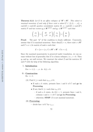
![Denote
qI Qt 0 qI
q= =
qI c 0 I qI c
and
M11 M12 I 0
Qt 0 M P Q 0 M21 M22 0 0
C= = .
0 I −P t 0 0 I
−I 0 0 0
0 0 0 0
Then the affine subspace E defined by
E = { (w, w∗ ) = ((yI , yI c ), (yI , yI c )) ∈ R n × R n : w∗ = Cw + q }
∗ ∗
tel-00675318, version 1 - 29 Feb 2012
is also maximal monotone.
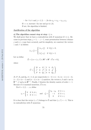
3.3 Construction of an affine maximal mono-
tone extension
Assume that E is an affine monotone, but not maximal monotone, subspace.
Then dim(E) < n, by Corollary 3.1.1 iii). We know that any monotone
subset has maximal monotone extensions, by the axiom of choice. But a
maximal extension of an affine subspace is not necessarily an affine subspace
as the following example shows.
Example 3.3.1 Consider E = { (x, x∗ ) ∈ R 2 × R 2 : Ax + Bx∗ = 0 }, where
A and B are the 3 × 2 matrices
1 −1 1 0
A = 1 −1
and B = 0 1 .
1 −1 0 0
The matrix C = [A, B] has rank 3. Easy computations lead to
2 0 1
t t
0 −2 −1
M = AB + BA =
1 −1 0
75](https://image.slidesharecdn.com/eladio-120609183205-phpapp02/85/Eladio-81-320.jpg)
![c)
and qI c ∈ R card (I such that
x∗ M P x I qI
(x, x∗ ) ∈ E =⇒ I = + .
xI c −P t 0 x∗ c
I qI c
Proof. By the previous construction, there exists a maximal monotone
affine subspace containing E. Apply Theorem 3.2.1.
Remark. The difference between Proposition 3.3.1 and Theorem 3.2.1 is
that the implication is one way for monotonicity and both ways for maximal
monotonicity.
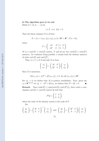
3.4 Restriction of an affine monotone sub-
tel-00675318, version 1 - 29 Feb 2012
space
In this section we assume that X = X ∗ = R n and U = U ∗ = R m and
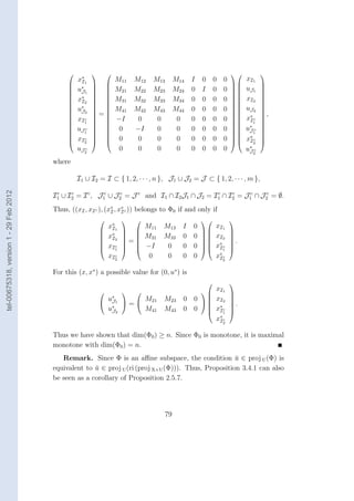
Φ ⊂ (X × U ) × (X ∗ × U ∗ ) is an affine subspace. As in section 2.4, given
u ∈ proj U Φ, we consider the subspace
¯
Φu = {(x, x∗ ) ∈ X × X ∗ : ∃ u∗ ∈ U ∗ such that ((x, u), (x∗ , u∗ )) ∈ Φ }.
¯ ¯
Proposition 3.4.1 Assume that Φ is (maximal) monotone. If we fixed u ∈
¯
proj U Φ. Then Φu is a (maximal) monotone affine subspace.
¯
Proof. Φ can be set as
Φ = { ((x, u), (x∗ , u∗ )) : Ax + Bu + Cx∗ + Du∗ = c },
where A and C are p×n matrices, B and D are p×m matrices and c ∈ R p . As
usual, we assume that c = 0 and that the matrix C = [A, B, C, D] has rank
p. For simplicity, we assume that u = 0. It is clear that the monotonicity
¯
of Φ0 follows from the monotonicity of Φ. Next, assume that Φ is maximal
monotone. By Theorem 3.1.1, p = n + m. Thanks to the remark just after
Theorem 3.2.1, we can assume that the linear subspace Φ is of the following
form
((xI , xI c , uJ , uJ c ), (x∗ , x∗ c , u∗ , u∗ c )) ∈ Φ if and only if
I I J J
78](https://image.slidesharecdn.com/eladio-120609183205-phpapp02/85/Eladio-84-320.jpg)


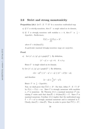
![4.1 The duality scheme for variational ine-
quality problems resulting from convex
optimization problems
In this section, we shall traduce the duality scheme for optimization problems
in terms of variational inequality problems. As in chapter 1, one considers
the problem:
Find x ∈ X such that f (¯) ≤ f (x), ∀ x ∈ X,
¯ x (P )
where f : X →] − ∞, +∞] is a proper lsc convex function. Next, let ϕ :
X × U →] − ∞, +∞] be a lsc convex function such that
tel-00675318, version 1 - 29 Feb 2012
ϕ(x, 0) = f (x), ∀ x ∈ X.
By construction ϕ is proper since dom (ϕ) ⊃ dom (f) × {0}. Next, for each
u ∈ U , define ϕu : X →] − ∞, +∞] by
ϕu (x) = ϕ(x, u), ∀ x ∈ X.
These functions are convex and lsc. The function ϕu is proper if and only if
u ∈ proj U (dom (ϕ)). The perturbed problems are:
Find xu ∈ X such that ϕu (¯u ) ≤ ϕu (x), ∀ x ∈ X.
¯ x (Pu )
Next, let F , Φ and Φu be the graphs of ∂f , ∂ϕ and ∂ϕu , respectively.
Since f , ϕ and ϕu are proper, convex and lsc functions, the sets F , Φ and
Φu are cyclically maximal monotone.
The problems (P ) and (Pu ) are respectively equivalent to the following
Variational Inequality Problems (VIP):
Find x ∈ X such that (¯, 0) ∈ F
¯ x (V )
and
Find xu ∈ X such that (¯u , 0) ∈ Φu .
¯ x (Vu ).
82](https://image.slidesharecdn.com/eladio-120609183205-phpapp02/85/Eladio-88-320.jpg)
![It is natural to say that problem (P ) ( (Pu ) ) is nondegenerate if the
function f ( ϕu ) is proper. Thus, we say that dom (f) and dom (ϕu ) are
the domains of nondegeneracy of (P ) and (Pu ), respectively. By analogy,
we say that the problems (V ) and (Vu ) are nondegenerate when F and Φu
are nonempty. The sets, proj X (F) and proj X (Φu ) are called the domains of
nondegeneracy of (V ) and (Vu ), respectively. Unfortunately, the domains of
nondegeneracy of (P) and (V) ( (Pu ) and (Vu ) ) do not coincide in general as
shown by the following example:
Example 4.1.1 Take X = R and define f : X →] − ∞, +∞] by
√
− x
if x ≥ 0,
f (x) =
tel-00675318, version 1 - 29 Feb 2012
+∞
otherwise.
Then, dom (f) = [ 0, +∞ [ and dom (F) = ] 0, +∞ [.
The following proposition is rather immediate.
Proposition 4.1.1 Assume that ϕ : X × U →] − ∞, +∞] is a proper lsc
convex function. Then
a) proj X (Φ) ⊂ proj X (dom(ϕ)).
b) ri (proj X Φ) = ri (proj X (dom(ϕ))), this set is convex.
c) cl (proj X Φ) = cl (proj X (dom (ϕ))), this set is convex.
d) proj U (Φ) ⊂ {u : proj X (Φu ) = ∅} = proj U (dom (ϕ)).
e) ri (proj U Φ) = ri ({u : proj X (Φu ) = ∅}) = ri (proj U (dom(ϕ))), this set
is convex.
f) cl (proj U Φ) = cl ({u : proj X (Φu ) = ∅}) = cl (proj U (dom(ϕ))), this
set is convex.
Proof.
83](https://image.slidesharecdn.com/eladio-120609183205-phpapp02/85/Eladio-89-320.jpg)
![a) By definition, x ∈ proj X (Φ) if and only if there exists u ∈ U such that
(x, u) ∈ dom (∂ϕ). This implies, in particular, that (x, u) ∈ dom (ϕ)
which is equivalent to say that x ∈ proj X (dom (ϕ)).
b) By (a), ri (proj X (Φ)) ⊂ ri (proj X (dom (ϕ))). The converse inclusion
follows from the relation ri (proj X (dom (ϕ))) = proj X (ri (dom (ϕ))),
which is due to the fact that the projection on a linear space is linear.
c) By (a), cl (proj X (Φ)) ⊂ cl (proj X (dom (ϕ))). On the other hand,
since cl (proj X (dom (ϕ))) = cl (ri (proj X (dom (ϕ)))), part b) implies
that cl (ri (proj X (dom (ϕ)))) = cl (ri (proj X (Φ))) ⊂ cl (proj X (Φ)), and
therefore the converse inclusion follows.
tel-00675318, version 1 - 29 Feb 2012
d) By definition, u ∈ proj U (Φ) if and only if there exists (x, x∗ , u∗ ) ∈ X ×
X ∗ × U ∗ such that (x∗ , u∗ ) ∈ ∂ϕ(x, u). This implies that x∗ ∈ ∂ϕu (x),
and therefore proj X (Φu ) = ∅. Next, assume that proj X (Φu ) = ∅.
Then there exists (x, x∗ ) ∈ X × X ∗ such that x∗ ∈ ∂ϕu (x). Hence
(x, u) ∈ dom (ϕ), and therefore u ∈ proj U (dom (ϕ)).
e) Similarly to b), ri (proj U (Φ)) = ri (proj U (dom (ϕ))). Thus, e) follows
from d).
f) Similarly to c), cl (proj U (Φ)) = cl (proj U (dom (ϕ))). Thus, f ) follows
from d).
The following proposition establishes a relation between Φ and Φu .
Proposition 4.1.2 Assume that ϕ : X × U →] − ∞, +∞] is a proper lsc
convex function. Then,
a) Φu ⊃ proj X×X∗ [Φ ∩ ((X × {u}) × (X∗ × U∗ ))];
b) If u ∈ ri (proj U Φ), then
Φu = proj X×X∗ [Φ ∩ ((X × {u}) × (X∗ × U∗ ))].
84](https://image.slidesharecdn.com/eladio-120609183205-phpapp02/85/Eladio-90-320.jpg)
. Next, define
x ¯ ¯ x
ψ : X × U →] − ∞, +∞] such that ψ(x, u) = ϕ(x, u) − x∗ , x . ψ is proper
¯
lsc and convex function. Associate with ψ the minimization problem
h(u) = inf ψ(x, u). (P1 )
x
Then, the dual optimization problem of (P1 ) is:
h∗∗ (u) = sup[ u∗ , u − ϕ∗ (¯∗ , u∗ )].
x (Q1 )
u∗
Since u ∈ ri (dom (h)), h(u) = h∗∗ (u) and ∂h(u) = ∅. Thus, for any u∗ ∈
¯
tel-00675318, version 1 - 29 Feb 2012
∂h(u),
ϕ(¯, u)− x∗ , x = min ψ(x, u) = sup[ u∗ , u −ϕ∗ (¯∗ , u∗ )] = u∗ , u −ϕ∗ (¯∗ , u∗ )
x ¯ ¯ x ¯ x ¯
x u∗
i.e.
(¯∗ , u∗ ) ∈ ∂ϕ(¯, u).
x ¯ x
This shows that
Φu ⊂ proj X×X∗ [Φ ∩ ((X × {u}) × (X∗ × U∗ ))],
and therefore the equality follows.
Remark. Since Φu is the graph of the subdifferential of a proper lsc
convex function, the sets ri (proj X (Φu )) and cl (proj X (Φu )) are convex when
u ∈ ri (proj U (Φ)). This is also the case when u ∈ proj U (Φ) because in
/
this case the two sets are empty. When u belongs to the boundary of the
projection of Φ on U , the following set
cl (proj X [Φ ∩ ((X × {u}) × (X∗ × U∗ ))])
may be not convex. This explains why b) does not hold in general.
Let us provide an example of such a situation.
85](https://image.slidesharecdn.com/eladio-120609183205-phpapp02/85/Eladio-91-320.jpg)
![Example 4.1.2 Take X = U = R. Define ϕ : X × U →] − ∞, +∞] by
√
max[ x2 , 1 − u ] if u ≥ 0,
ϕ(x, u)
+∞
if not.
The function ϕ is proper convex and lsc (see example 1.2.1). Take u = 0.
Then,
Φ0 = { (x, 2x) : |x| > 1 }∪({−1}×[ −2, 0 ])∪{ (x, 0) : |x| < 1 }∪({1}×[ 0, 2 ])
and
proj X×X∗ [Φ ∩ ((X × {0}) × (X∗ × U∗ ))] = { (x, 2x) : |x| ≥ 1 }.
tel-00675318, version 1 - 29 Feb 2012
Hence
ri (proj X (Φ0 )) = cl (proj X (Φ0 )) = X
and
cl (proj X [Φ ∩ ((X × {0}) × (X∗ × U∗ ))]) = X ] − 1, +1[.
The first set is convex, but the second one is not. In this example u = 0
belongs to the boundary of proj U (Φ).
According to Proposition 4.1.2, when 0 ∈ ri (proj U (Φ)) (u ∈ ri (proj U (Φ))),
the variational inequality problem (V) ((Vu )) can be formulated as
Find x ∈ X such that ∃ u∗ ∈ U ∗ with (x, 0, 0, u∗ ) ∈ Φ, (V 0 )
( Find xu ∈ X such that ∃ u∗ ∈ U ∗ with (xu , u, 0, u∗ ) ∈ Φ). (V u )
Next, we shall consider a dual formulation of problem (V). Here, again
we refer the duality scheme in optimization problem.
The dual optimization problem associated to (P ) is
Find u∗ ∈ U ∗ such that d(¯∗ ) ≤ d(u∗ ), ∀ u∗ ∈ U ∗ ,
¯ u (D)
where the function d : U ∗ → [−∞, +∞] is defined by
d(u∗ ) = ϕ∗ (0, u∗ ) = ϕ∗ (u∗ ), ∀ u∗ ∈ U ∗ .
0
86](https://image.slidesharecdn.com/eladio-120609183205-phpapp02/85/Eladio-92-320.jpg)
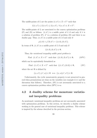
![The variational formulation of (D) is
Find u∗ ∈ U ∗ such that (0, u∗ ) ∈ G,
¯ ¯ (DV )
where
G− = graph (∂d) = graph (∂ϕ0 ).
∗
We say that (DV) is a dual variational inequality problem associated to (V ).
Assume that 0 ∈ ri (proj X∗ (Φ)). Then, in the same way that we have
done for the primal problems (V) and (V0 ), we reformulate (DV) in terms of
Φ as
Find u∗ ∈ U ∗ such that ∃ x ∈ X with (x, 0, 0, u∗ ) ∈ Φ.
¯ (DV 0 )
tel-00675318, version 1 - 29 Feb 2012
Also, the perturbed variational inequality problems associated to (DV)
are
Find u∗ ∈ U ∗ such that (0, u∗ ) ∈ Gx∗ ,
¯ ¯ (DVx∗ )
where (Gx∗ )− = graph (∂ϕ∗∗ ) and the function ϕ∗ ∗ is defined by
x x
ϕ∗ ∗ (u∗ ) = ϕ∗ (x∗ , u∗ ), ∀ u∗ ∈ U ∗ .
x
Here, the elements x∗ belonging to proj X∗ (Φ) are taken as the dual pertur-
bation parameters.
The dual perturbed optimization problems associated to (D) are
Find u∗ ∗ ∈ U ∗ such that ϕ∗ ∗ (¯∗ ∗ ) ≤ ϕ∗ ∗ (u∗ ∗ ), ∀ u∗ ∈ U ∗ ,
¯x x ux x x (Dx∗ )
which, if x∗ ∈ ri (proj X∗ (Φ)), are equivalent, in terms of Φ, to:
∗
Find u∗ ∗ ∈ U ∗ such that ∃ x ∈ X with (x, 0, x∗ , u∗ ∗ ) ∈ Φ.
¯x ¯x (DV x )
Our next step consists in giving a variational inequality formulation for
the lagrangian. Recall that the lagrangian function L : X × U ∗ → [−∞, +∞]
associated to the perturbation function ϕ : X × U →] − ∞, +∞] is defined
by
L(x, u∗ ) = inf [ −u, u∗ + ϕ(x, u) ].
u∈U
87](https://image.slidesharecdn.com/eladio-120609183205-phpapp02/85/Eladio-93-320.jpg)
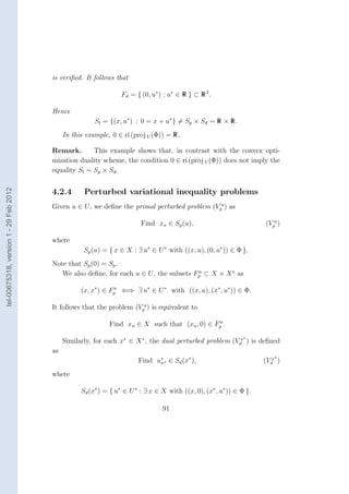
![Example 4.2.2 (see Example 4.1.2) Consider for Φ, the graph of the sub-
differential of the function ϕ : X × U →] − ∞, +∞] defined by
√
max[ x2 , 1 − u ]
if u ≥ 0,
ϕ(x, u) =
+∞
if not.
Then
Fp = {(x, 2x) : |x| ≥ 1},
which is monotone but not maximal monotone. In this particular example,
0 ∈ bd (proj U (Φ)).
tel-00675318, version 1 - 29 Feb 2012
Linear and convex quadratic programming are two cases where the con-
vex optimization duality scheme works with minimal assumptions. The cor-
responding case in our scheme is the case where Φ is affine.
Proposition 4.2.2 Assume that Φ is a maximal monotone affine subspace
x∗
and (u, x∗ ) ∈ proj U (Φ) × proj X∗ (Φ). Then, the sets Fp and Fd are maximal
u
monotone affine subspace and solutions sets Sl , Sp (u) and Sd (x∗ ) are also
affine subspaces.
Proof. The assumptions are equivalent to assumptions in Proposition 3.4.1,
u x∗
so, we deduce that Fp and Fd are maximal monotone affine subspaces. On
the other hand, by definition, for all (x∗ , u) ∈ X ∗ × U , the sets Λ(x∗ , u) are
affine subspaces. Thus, the sets Sl , Sp (u) and Sd (x∗ ) are affine subspaces,
because, by (4.1), are projection of affine subspaces.
For the treatment of the nonaffine case, the following classical result is
useful, see for instance [10].
Proposition 4.2.3 Given f : R n → R p linear and C ⊂ R n such that ri (C)
and cl (C) are convex. If ri (cl (C)) = ri (C), then f (ri (C)) = ri (f(C)).
The projection onto a linear space is linear. We obtain the following results
on primal and dual problems.
93](https://image.slidesharecdn.com/eladio-120609183205-phpapp02/85/Eladio-99-320.jpg)
![As a simple consequence of these last results we have the following:
Corollary 4.2.1 With the same assumption of Proposition 4.2.4 or Proposi-
tion 4.2.5, we have that Sp (0) is convex, compact and not empty if and only if
Sd (0) it so. Furthermore, there exists an open neighborhood N ×W ⊂ U ×X ∗
x∗
of (0, 0), such that, for each (u, x∗ ) ∈ N × W , the subsets Fp and Fd are
u
maximal monotone.
Next, we shall study the behavior of the primal and dual perturbed prob-
lems in a neighborhood of u = 0.
Theorem 4.2.1 Assume that Φ ⊂ (X ×U )×(X ∗ ×U ∗ ) is maximal monotone
and (0, 0) ∈ int (dom (Λ)). Then, there exist K, a compact subset of X, T ,
tel-00675318, version 1 - 29 Feb 2012
a compact subset of U ∗ , V , an open convex neighborhood of 0 in U , and W ,
an open convex neighborhood of 0 in X ∗ , such that
a) For all (u, x∗ ) ∈ V × W , ∅ = Sp (u) ⊂ K and ∅ = Sd (x∗ ) ⊂ T .
b) The multivalued maps Sp and Sd are usc on V and W , respectively.
Proof. By assumption, the multivalued map Λ is maximal monotone and
(0, 0) ∈ int (dom (Λ)), from what we deduce that a compact subset K of X,
a compact subset T of U ∗ , an open convex neighborhood V of 0 in U , and
an open convex neighborhood W of 0 in X ∗ exist, satisfying
∅ = Λ(x∗ , u) ⊂ K × T, ∀ (x∗ , u) ∈ W × V.
By (4.1),
Sp (u) = proj X [Λ(0, u)] and Sd (x∗ ) = proj U∗ [Λ(x∗ , 0)],
from what we obtain, for all (x∗ , u) ∈ W × V ,
∅ = Sp (u) ⊂ K and ∅ = Sd (x∗ ) ⊂ T.
Hence a) follows.
Next, the upper semicontinuity in b) follows from the fact that Λ is usc
on W × V and the projections proj X and proj U∗ are continuous functions.
96](https://image.slidesharecdn.com/eladio-120609183205-phpapp02/85/Eladio-102-320.jpg)
![Proposition 4.2.11 Assume that Φ ⊂ (X × U ) × (X ∗ × U ∗ ) is maxi-
mal monotone and (0, 0) ∈ ri (dom (Λ)). Denotes by Lp and Ld the par-
allel subspace to aff (proj X∗ (F0 )) = aff (dom (Σp )) and aff (proj U (F0 )) =
p d
aff (dom (Σd )), respectively. Then, there exist K, a compact subset of X, T ,
a compact subset of U ∗ , V , a relative open convex neighborhood of 0 in U ,
and W , a relative open convex neighborhood of 0 in X ∗ such that
a) For all (u, x∗ ) ∈ V × W , ∅ = Sp (u) = Sp (u) + Lp ⊂ K + Lp and
⊥ ⊥
∅ = Sd (x∗ ) = Sd (x∗ ) + L⊥ ⊂ T + L⊥ .
d d
b) The multivalued maps Sp and Sd are usc on V and W , respectively.
Proof. By assumption, Λ is maximal monotone and (0, 0) ∈ ri (dom(Λ)).
Denote by L, the affine hull of dom (Λ). Then
tel-00675318, version 1 - 29 Feb 2012
L = { (x∗ , u) ∈ X ∗ × U : Ax∗ + Bu = 0 },
for some matrices A and B of appropriate order. This implies that
L⊥ = img ([A, B]t ), proj X (L⊥ ) = L⊥
p and proj U∗ (L⊥ ) = L⊥ .
d (4.2)
By Proposition 2.5.4, there exist a compact subset K of X, a compact subset
T of U ∗ , an open convex neighborhood V of 0 in U and an open convex
neighborhood W of 0 in X ∗ exist satisfying
∅ = Λ(x∗ , u) = Λ(x∗ , u) + L⊥ ⊂ K × T + L⊥ , ∀ (x∗ , u) ∈ W × V. (4.3)
By (4.1),
Sp (u) = proj X [Λ(0, u)] and Sd (x∗ ) = proj U∗ [Λ(x∗ , 0)].
Relations (4.2) and (4.3) imply that for all (u, x∗ ) ∈ V × W ,
⊥ ⊥
∅ = Sp (u) = Sp (u) + Lp ⊂ K + Lp
and
∅ = Sd (x∗ ) = Sd (x∗ ) + Ld ⊂ T + Ld ,
⊥ ⊥
from the what a) is verified. On the other hand, since the multivalued map
Λ is usc on W × V and the projections proj X and proj U∗ are continuous
functions, the upper semicontinuity in b) is verified.
99](https://image.slidesharecdn.com/eladio-120609183205-phpapp02/85/Eladio-105-320.jpg)

![b) Assume now that Γ1 and Γ2 are maximal monotone. Let us consider
−→
the multivalued map Σ : U ∗ × X −→ U × X ∗ defined by
Σ(u∗ , x) = {(u, x∗ ) : ((x, u), (x∗ , u∗ ) ∈ Φ}.
Then,
Σ(u∗ , u∗ , x) = [Γ− (u∗ ) − x] × [Γ− (u∗ ) − x] × {u∗ + u∗ },
1 2 1 1 2 2 1 2
and
dom (Σ) = dom (Γ− ) × dom (Γ− ) × X.
1 2
Since the graph of Σ corresponds to Φ after permutation of variables, Φ
is maximal monotone if and only if Σ is maximal monotone. For this, by
Proposition 2.1.1, it is enough to prove that
tel-00675318, version 1 - 29 Feb 2012
Σ(u∗ , u∗ , x) = [Γ− (u∗ ) − x] × [Γ− (u∗ ) − x] × {u∗ + u∗ }.
1 2 1 1 2 2 1 2
Assume that (u1 , u2 , x∗ ) ∈ Σ(u∗ , u∗ , x). Then, for all (v1 , v1 ) ∈ graph (Γ1 ),
1 2
∗
∗
(v2 , v2 ) ∈ graph (Γ2 ) and y ∈ X, one has B ≥ 0, where
B = u∗ − v1 , u1 − v1 + y + u∗ − v2 , u2 − v2 + y + x∗ − v1 − v2 , x − y .
1
∗
2
∗ ∗ ∗
Easy computations give
B = u∗ − v1 , u1 − v1 + u∗ − v2 , u2 − v2 + x∗ − v1 − v2 , x − x∗ − u∗ − u∗ , y .
1
∗
2
∗ ∗ ∗
1 2
∗ ∗
Let (v1 , v1 ) ∈ graph (Γ1 ) and (v2 , v2 ) ∈ graph (Γ2 ) be fixed. Since B ≥ 0 for
all y ∈ X, one obtains
x ∗ = u∗ + u∗ .
1 2
Using this identity for x∗ in the last expression of B, we see that
u∗ − vi , (ui + x) − vi ≥ 0, ∀(vi , vi ) ∈ graph (Γi ), i = 1, 2.
i
∗ ∗
i=1,2
Assume for contradiction that u1 + x ∈ Γ− (u∗ ), then there exists (v1 , v1 ) ∈
/ 1 1 ∗
graph (Γ1 ) so that u∗ −v1 , (u1 +x) −v1 < 0 and consequently u∗ −v2 , (u2 +
1
∗
2
∗
∗
x) − v2 > 0 whenever (v2 , v2 ) ∈ graph (Γ2 ). One deduces that u2 + x ∈
Γ− (u∗ ). Next, take (v2 , v2 ) = (u2 +x, u∗ ), then one has u∗ −v2 , (u2 +x)−v2 =
2 2
∗
2 2
∗
0 in contradiction with the inequality above.
One obtains that Σ is maximal monotone.
103](https://image.slidesharecdn.com/eladio-120609183205-phpapp02/85/Eladio-109-320.jpg)
![and
proj X∗ ×U (Φ) = { (¯1 − x, u2 − x, u∗ + u∗ ) : x ∈ X, u∗ ∈ dom (Γ− ), i = 1, 2 },
u ¯ 1 2 i i
which, obviously, has empty interior.
Next, we will specialize the conditions in Theorem 4.2.1 in order to es-
tablish the stability property of primal and dual perturbed problems.
In the following proposition, which is rather immediate, one assumes that
the multivalued maps Γ = Γ1 + Γ2 and Σ = Σ1 + Σ2 are maximal monotone,
where Σ1 and Σ2 are defined by Σ1 ≡ Γ1 and Σ2 (v ∗ ) = −Γ− (−v ∗ ), ∀ v ∗ ∈
−
2
∗
X .
tel-00675318, version 1 - 29 Feb 2012
Proposition 5.1.6 In the following six statements, we have the following
equivalences: a ⇔ b ⇔ c and a ⇔ b ⇔ c .
a) The solution set Sp (0) is bounded and not empty.
b) 0 ∈ int (img (Γ)).
− ∗ − ∗ ∗
c) ∃ W ∈ N (0) such that v ∗ ∈X ∗ [Γ1 (v ) ∩ Γ2 (x − v )] = ∅, ∀ x∗ ∈ W .
a’) The solution set Sd (0) is bounded and not empty.
b’) 0 ∈ int (img (Σ)).
c’) ∃ V ∈ N (0) such that z∈X [Γ1 (z) ∩ −Γ2 (z − x)] = ∅, ∀x ∈ V .
Applying Proposition 4.2.1 and Theorem 4.2.1, one obtains that, under
ˆ ˆ
conditions b) ( or c) and b ) (or c ), there exist an open neighborhood V × W ⊂
∗ ∗
U × X of (0, 0) and a compact K × L ⊂ X × U such that:
• ∅ = Sp (u) ⊂ K and ∅ = Sd (x∗ ) ⊂ L, ˆ ˆ
∀ (u, x∗ ) ∈ V × W
ˆ ˆ
• The multivalued maps Sp and Sd are usc on V and W , respectively.
108](https://image.slidesharecdn.com/eladio-120609183205-phpapp02/85/Eladio-114-320.jpg)
![Define Φ ⊂ (X × U ) × (X ∗ × U ∗ ) as:
Φ = {((x, u1 , u2 ), (x∗ , u∗ , u∗ )) : u∗ ∈ Γ1 (x + u1 ), u∗ = x∗ − u1 ∈ NC (x + u2 )}.
1 2 1 2
∗
Since, by assumption, Γ1 and Γ2 are maximal monotone, Proposition 5.1.1
implies that Φ is maximal monotone and, therefore, the monotonicity of Fp .
The dual problem.
According to our duality scheme, the subset Fd , in this case becomes
Fd = { (u, u∗ ) : ∃ x ∈ X s.t. u∗ ∈ Γ1 (x + u1 ) and u∗ = −u∗ ∈ NC (x + u2 ) },
1 2 1
tel-00675318, version 1 - 29 Feb 2012
which, by the monotonicity of Φ, is also monotone.
The dual VIP problem can be equivalently formulated as:
∃ x ∈ X with u∗ ∈ Γ (x)
¯1 1
Find u∗ = (¯∗ , u∗ ) ∈ U ∗ such that
¯ u1 ¯ 2 ∗ ∗
(Vd )
and u = −u ∈ NC (x),
¯ 2 1
Find u∗ ∈ X ∗ such that Γ− (¯∗ ) ∩ NC (−¯∗ ) = ∅
¯ 1 u
−
u (Vd )
or again
Find u∗ ∈ X ∗ such that 0 ∈ Γ− (¯∗ ) − NC (−¯∗ ).
¯ 1 u
−
u (Vd )
−
Since NC (0) = C, the second one of these formulations of (Vd ) implies in
particular that
0 ∈ Γ1 (C) ⇐⇒ 0 is a solution of problem (Vd ).
The third one of these formulations is a dual framework studied by Mosco,
in [27].
The perturbed problems and the lagrangian problem.
u
Given the perturbation variable u ∈ X × X, the subset Fp is
Fp = { (x, x∗ ) : x∗ ∈ Γ1 (x + u1 ) + NC (x + u2 ) },
u
110](https://image.slidesharecdn.com/eladio-120609183205-phpapp02/85/Eladio-116-320.jpg)
![Since NC ∗ (0) = C, the second one of these formulations of (Vd ) implies
in particular that
0 ∈ Γ1 (C) ⇐⇒ 0 is a solution of problem (Vd ).
The perturbed problems and the lagrangian problem.
u
Given the perturbation variable u ∈ X × X, the subset Fp is
Fp = { (x, x∗ ) : x∗ ∈ Γ1 (x + u1 ) + NC (x + u2 ) },
u
and therefore, the primal perturbed problem (Vpu ) becomes
Find x ∈ X such that 0 ∈ Γ1 (¯ + u1 ) + NC (¯ + u2 ).
¯ x x (Vpu )
tel-00675318, version 1 - 29 Feb 2012
∗
Next, given the perturbation variable x∗ ∈ X ∗ , the subset Fd is
x
x∗
∃ x ∈ X with u∗ + u∗ = x∗ ,
Fd = (u, u∗ ) : ∗ 1 2
u1 ∈ Γ1 (x + u1 ) and u∗ ∈ NC (x + u2 )
2
or, equivalently,
∗
Fd = { (u, u∗ ) : [Γ− (u∗ ) − u1 ] ∩ [NC ∗ (u∗ ) − u2 ] = ∅ and u∗ + u∗ = x∗ },
x
1 1 2 1 2
∗
and therefore, the dual perturbed problem (Vdx ) becomes
∃ x ∈ X with u∗ ∈ Γ1 (x)
¯1 ∗
Find u∗ = (¯∗ , u∗ ) ∈ U ∗ such that
¯ u1 ¯ 2 (Vdx )
and u∗ = x∗ − u∗ ∈ NC (x),
¯2 1
which can be equivalently formulated as
∗
Find u∗ ∈ X ∗ such that Γ− (¯∗ ) ∩ NC ∗ (x∗ − u∗ ) = ∅
¯ 1 u ¯ (Vdx )
∗
Find u∗ ∈ X ∗ such that 0 ∈ Γ− (¯∗ ) + NC + (¯∗ − x∗ )
¯ 1 u u (Vdx )
∗
Find u∗ ∈ C + such that ∃ u ∈ Γ− (¯x∗ +x∗ )∩C with ux∗ , u = 0. (Vdx )
¯ ¯ 1 u ¯ ¯
Again, by the fact that NC ∗ (0) = C, the second one of these formulations of
∗
(Vdx ) implies in particular that
∗
w∗ ∈ Γ1 (C) ⇐⇒ w∗ is a solution of problem (Vdw ).
114](https://image.slidesharecdn.com/eladio-120609183205-phpapp02/85/Eladio-120-320.jpg)
![The perturbed problems and the lagrangian problem.
u
Given the perturbation variable u ∈ X × X, the subset Fp is
Fp = { (x, x∗ ) : x∗ ∈ Γ1 (x + u1 ) + NR n (x + u2 ) },
u
+
and therefore, the primal perturbed problem (Vpu ) becomes
Find x ∈ X such that 0 ∈ Γ1 (¯ + u1 ) + NR n (¯ + u2 ).
¯ x +
x (Vpu )
∗
Next, given the perturbation variable x∗ ∈ X ∗ , the subset Fd is
x
∗
x∗
∃ x ∈ X with u1
+ =x ,u∗ ∗
Fd = (u, u∗ ) : ∗ ∗
2
u1 ∈ Γ1 (x + u1 ) and u2 ∈ NR n (x + u2 )
+
tel-00675318, version 1 - 29 Feb 2012
or equivalently
∗
Fd = { (u, u∗ ) : [Γ− (u∗ ) − u1 ] ∩ [NR n (u∗ ) − u2 ] = ∅ and u∗ + u∗ = x∗ },
x
1 1 − 2 1 2
∗
and therefore, the dual perturbed problem (Vdx ) becomes
∃ x ∈ X with u∗ ∈ Γ1 (x)
¯1 ∗
Find u∗ = (¯1 , u∗ ) ∈ U ∗ s.t.
¯ u∗ ¯ 2 (Vdx )
and u = x − u∗ ∈ NR n (x),
∗
¯2 ∗
1 +
which can be equivalently formulated as
∗
Find u∗ ∈ X ∗ such that Γ− (¯∗ ) ∩ −NR n (¯∗ − x∗ ) = ∅
¯ 1 u +
u (Vdx )
∗
Find u∗ ∈ X ∗ such that 0 ∈ Γ− (¯∗ ) + NR n (¯∗ − x∗ )
¯ 1 u +
u (Vdx )
∗
Find u∗ ∈ R n such that ∃ u ∈ Γ− (¯x∗ +x∗ )∩R n with ux∗ , u = 0. (Vdx )
¯ + ¯ 1 u + ¯ ¯
∗
Again, the second one of these formulations of (Vdx ) implies in particular
that
∗
w∗ ∈ Γ1 (R n ) ⇐⇒ w∗ is a solution of problem (Vdw ).
+
Finally, the multivalued map Λ becomes
Λ(x∗ , u) = { (x, u∗ ) : u∗ ∈ Γ1 (x + u1 ), u∗ ∈ NR n (x + u2 ) and u∗ + u∗ = x∗ },
1 2 + 1 2
117](https://image.slidesharecdn.com/eladio-120609183205-phpapp02/85/Eladio-123-320.jpg)
![and therefore, the problem (VL ) is formulated as:
u∗ ∈ Γ1 (¯) and
¯1 x
Find (¯, u∗ ) ∈ X × U ∗ such that
x ¯ ∗ ∗
(VL )
u = −¯ ∈ NR n (¯).
¯2 u1 x
+
∗
In this particular example, the solutions sets of problems (Vpu ), (Vdx ) and
(VL ), become:
Sp (u) = {x ∈ X : 0 ∈ Γ1 (x + u1 ) + NR n (x + u2 ) },
+
Sd (x∗ ) = {(v ∗ , x∗ − v ∗ ) ∈ U ∗ : 0 ∈ Γ− (v ∗ ) + NR n (v ∗ − x∗ ) }
1 +
and
Sl = {(x, (v ∗ , −v ∗ )) ∈ X × U ∗ : v ∗ ∈ Γ1 (x) and − v ∗ ∈ NR n (x) }.
tel-00675318, version 1 - 29 Feb 2012
+
Sensitivity and stability analysis.
In the present case, conditions (Dsp), (Dwp), (Dsd) and (Dwd) are:
int (dom (Γ1 ))) ∩ int (R n ) = ∅,
+ (Dsp)
ri (dom (Γ1 ))) ∩ int (R n ) = ∅,
+ (Dwp)
dom (Γ− ) ∩ int (R n ) = ∅.
1 + (Dsd) = (Dwd)
5.2.4 The Auslender-Teboulle lagrangian duality
In this example consider C = ∩r Ck , where Ck is the closed convex set
k=1
defined by Ck = { x ∈ X : gk (x) ≤ 0 }, with gk given proper lsc convex
function. Denote NCk the normal cone to Ck .
Again, assume that the multivalued map Γ1 is maximal monotone and
dom (Γ1 ) ∩ C = ∅.
By duality in linear programming, a vector x∗ belongs to NCk (x) if and
only if gk (x) ≤ 0 and there exists a real number µ∗ ≥ 0 for which x∗ =
k
µ∗ ∂gk (x) and µ∗ gk (x) = 0.
k k
Then (see [35], Corollary 28.2.1) under Slater’s condition
∃ x ∈ X such that gk (x) < 0, k = 1, 2, · · · , r, (5.1)
118](https://image.slidesharecdn.com/eladio-120609183205-phpapp02/85/Eladio-124-320.jpg)
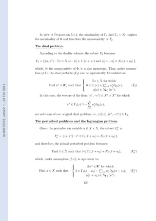
![∗
Next, given the perturbation variable x∗ ∈ X ∗ , the subset Fd is
x
∗
Fd = { (u, u∗ ) : [Γ− (u∗ ) − u1 ] ∩ [NC (u∗ ) − u2 ] = ∅ and u∗ + u∗ = x∗ }
x
1 1
−
2 1 2
and, therefore, the dual perturbed problem becomes:
∗
Find u∗ ∈ U ∗ such that [Γ− (u∗ )] ∩ [NC (u∗ )] = ∅ and u∗ + u∗ = x∗ , (Vdx )
¯ 1 1
−
2 1 2
which, under assumption (5.1), is equivalent to:
∃ x ∈ X for which
∗
Find w ∈ ∗
Rr such that x ∈ Γ1 (x) + r wj ∂gj (x),
∗ ∗ ˆ
(Vdx )
+ j=1
g(x) ∈ NR r (w∗ ).
+
In this case, vectors of the form (v ∗ , −v ∗ ) ∈ X ∗ × X ∗ for which
tel-00675318, version 1 - 29 Feb 2012
r
v ∗ ∈ [Γ1 (x) − x∗ ] ∩ − ∗
wj ∂gj (x),
j=1
∗
are such that, ((0, 0), (v ∗ , −v ∗ )) ∈ Fd .
x
−→
Finally, the multifunction Λ : X ∗ × U −→ X × U ∗ is defined by
Λ(x∗ , u) =
{ (x, u∗ ) ∈ X × U ∗ : u∗ ∈ Γ1 (x + u1 ), u∗ ∈ NC (x + u2 ) and u∗ + u∗ = x∗ }
1 2 1 2
and therefore, the lagrangian problem becomes
u∗ ∈ Γ1 (¯) and
¯1 x
Find (¯, u∗ ) ∈ X × U ∗ such that
x ¯ ∗ ∗
(VL )
u = −¯ ∈ NC (¯),
¯2 u1 x
which, under assumption (5.1), is equivalent to:
0 ∈ Γ (x) + r w ∗ ∂g (x),
1 j ˆ
Find (x, w∗ ) ∈ X × R r
+ such that j=1 j
(VL )
r (w ∗ ).
g(x) ∈ NR +
In this case, the vectors of the form (x, (v ∗ , −v ∗ )) ∈ X × U ∗ , for which
r
v ∗ ∈ [Γ1 (x)] ∩ − ∗
wj ∂gj (x),
j=1
121](https://image.slidesharecdn.com/eladio-120609183205-phpapp02/85/Eladio-127-320.jpg)
![belong to Λ(0, 0).
ˆ ˆ ˆ
The formulations of problems (Vp ), (Vd ) and (VL ) are, respectively, the
well known formulations of primal problem, dual problem, and primal-dual
problem developed by Auslender and Teboulle, in [2].
5.3 Sum of more that two monotone maps
In this section we shall apply our duality scheme to the sum of more that
two monotone maps. Thus, this section can be seen as a generalization of
Section 5.1.
Consider X = X ∗ = R n and for i = 1, 2, · · · , q, Yi = Yi∗ = R ri and the
tel-00675318, version 1 - 29 Feb 2012
−→
multivalued maps Γi : Yi −→ Yi∗ .
−→
Define Γ : X −→ X ∗ by
q
Γ(x) = At Γi (Ai x + ai ),
i
i=1
where for i = 1, 2, · · · , q, Ai is a ri × n surjective matrix and ai ∈ R ri .
It is clear that if the multivalued maps Γi , i = 1, 2, · · · , q, are monotone,
then the multivalued map Γ is also monotone.
We shall apply the duality scheme to the following problem
Find x ∈ X such that 0 ∈ Γ(¯).
¯ x (V )
Assume that dom (Γ) is not empty. Denote Fp = graph (Γ), then
for i = 1, 2, · · · , q, ∃ yi ∈ Yi∗ with
∗
Fp = (x, x∗ ) : ∗
yi ∈ Γi (Ai x + ai ) and q At yi = x∗
i=1 i
∗
and therefore the problem (V ) can be written as
Find x ∈ X such that (¯, 0) ∈ Fp .
¯ x (Vp )
122](https://image.slidesharecdn.com/eladio-120609183205-phpapp02/85/Eladio-128-320.jpg)
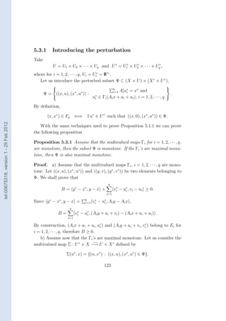
![Then,
q
Σ(u∗ , · · · , u∗ , x) = [Γ− (u∗ )−A1 x−a1 ]×· · ·×[Γ− (u∗ )−Aq x−aq ]×{
1 q 1 1 q q At u∗ }.
i i
i=1
Since the graph of Σ corresponds to Φ after permutation of variables, Φ is
maximal monotone if and only if Σ is maximal monotone. For this, it is
enough to prove that
q
Σ(u∗ , · · · , u∗ , x) = [Γ− (u∗ )−A1 x−a1 ]×· · ·×[Γ− (u∗ )−Aq x−aq ]×{
1 q 1 1 q q At u∗ }.
i i
i=1
Assume that (u1 , u2 , · · · , uq , x∗ ) ∈ Σ(u∗ , u∗ , · · · , u∗ , x). Then, for all (vi , vi ) ∈
1 2 q
∗
graph (Γi ), i = 1, 2, · · · , q and y ∈ X one has, B ≥ 0, where
tel-00675318, version 1 - 29 Feb 2012
q q
B= u∗
i − ∗
vi , ui + Ai y + a i − v i + x − ∗
i
∗
At v i , x − y .
i=1 i=1
Easy computations give
q q q
B= u∗
i − ∗
vi , ui + ai − v i + x − ∗
i
∗
At v i , x + At u i − x ∗ , y ,
i
∗
i=1 i=1 i=1
from what q
x∗ = At u ∗ .
i i
i=1
Using this relation in the last expression of B, we see that
q
u∗ − vi , (ui + Ai x + ai ) − vi ≥ 0, ∀(vi , vi ) ∈ graph (Γi ), i = 1, 2 · · · , q.
i
∗ ∗
i=1
Assume for contradiction that u1 + x ∈ Γ− (u∗ ), then there exists (v1 , v1 ) ∈
/ 1 1 ∗
graph (Γ1 ) satisfying u∗ − v1 , (u1 + x) − v1 < 0 and consequently, for some
1
∗
i
∗ ∗
index i = 1, u∗ − vi , (ui + Ai x + ai ) − vi > 0 whenever (vi , vi ) ∈ graph (Γi ).
One deduces that ui + Ai x + ai ∈ Γ− (u∗ ). Next, take (vi , vi ) = (ui + Ai x +
i i
∗
i i
∗
ai , u∗ ), then one has u∗ − vi , (ui + Ai x + ai ) − vi = 0 in contradiction with
the inequality above.
One obtains that Σ is maximal monotone.
124](https://image.slidesharecdn.com/eladio-120609183205-phpapp02/85/Eladio-130-320.jpg)
![5.3.2 The dual problem
According to the duality scheme, the subset Fd is defined by the relation
(u, u∗ ) ∈ Fd ⇐⇒ ∃ x ∈ X such that ((x, u), (0, u∗ )) ∈ Φ,
in the present case,
∃ x ∈ X such that q At ui = 0 and
∗
Fd = (u, u∗ ) : i=1 i
.
u∗ ∈ Γi (Ai x + ai + ui ), i = 1, 2, · · · , q
i
The dual problem is formulated as:
tel-00675318, version 1 - 29 Feb 2012
∃ x ∈ X with q t ∗
i=0 Ai ui = 0 and
¯
Find u∗ ∈ U ∗ such that ∗
¯ (Vd )
u ∈ Γi (Ai x + ai ), i = 0, 1, · · · , q,
¯ i
which can also be formulated as
q q
Find u∗ ∈ U ∗ s.t
¯ At u∗ = 0 and
i ¯i [A† (Γ− (¯∗ ) − ai ) + ker(Ai )] = ∅,
i i ui
i=1 i=1
where A† denotes the Moore-Penrose pseudoinverse of matrix A, which, if A
is surjective, has the expression A† = At (AAt )−1 .
5.3.3 The perturbed problems and the lagrangian pro-
blem
u
Given the perturbation variable u ∈ X × X, the subset Fp is
for i = 1, 2, · · · , q, ∃ yi ∈ Yi∗ with
∗
Fp = (x, x∗ ) : ∗
u
yi ∈ Γi (Ai x + ai + ui ) and q At yi = x∗
i=1 i
∗
and therefore the primal perturbed problem (Vpu ) can be written as
for i = 0, 1, · · · , q, ∃ yi ∈ Y ∗ with
∗
Find xu ∈ X s.t
¯ q (Vpu )
y ∗ ∈ Γi (Ai xu + ai + ui ) and
¯ t ∗
i i=0 Ai yi = 0.
125](https://image.slidesharecdn.com/eladio-120609183205-phpapp02/85/Eladio-131-320.jpg)
![∗
Next, given the perturbation variable x∗ ∈ X ∗ , the subset Fd is
x
q ∗ ∗
∗
∃ x ∈ X such that At u i
= x and
Fd = (u, u∗ ) :
x i=1 i
u∗ ∈ Γi (Ai x + ai + ui ), i = 1, 2, · · · , q
i
and therefore, the dual perturbed problem becomes:
∃ x ∈ X with q t ∗ ∗
∗ ∗ i=0 Ai ui = x and
¯ ∗
Find u ∈ U such that
¯ (Vdx )
u∗ ∈ Γi (Ai x + ai ), i = 0, 1, · · · , q,
¯ i
which is equivalent to
q q
At u ∗ ∗
[A† (Γi (¯∗ ) − ai ) + ker(Ai )] = ∅.
−
tel-00675318, version 1 - 29 Feb 2012
Find xu ∈ X s.t.
¯ i ¯i = x and i ui
i=1 i=1
−→
Finally, the multifunction Λ : X ∗ × U −→ X × U ∗ is defined by
q
At u∗ = x∗ and
Λ(x∗ , u) = (x, u∗ ) : ∗ i i i=1
ui ∈ Γi (Ai x + ai + ui ), i = 1, 2, · · · , q
and therefore, the Lagrangian problem becomes
q
∗ ∗
At u∗ = 0 and
i ¯i
i=1
Find (¯, u ) ∈ X × U s.t.
x ¯ (VL )
u∗ ∈ Γi (Ai x + ai ), i = 1, 2, · · · , q.
¯i ¯
5.3.4 Sensitivity and stability analysis
In this general case, let us consider the following conditions:
Γ1 , Γ2 · · · , Γq are maximal monotone (M m)
q
{ x ∈ X : Ai x + ai ∈ int (dom (Γi )) } = ∅ (Dsp)
i=1
and the weaker form
q
{ x ∈ X : Ai x + ai ∈ ri (dom (Γi )) } = ∅. (Dwp)
i=1
126](https://image.slidesharecdn.com/eladio-120609183205-phpapp02/85/Eladio-132-320.jpg)
![We have already seen that condition (M m) implies that Φ is maximal
monotone, hence Sl is closed and convex. Similarly to Proposition 5.1.2, we
obtain the following sufficient condition in order to establish the maximality
u
of Fp , for u belonging in some open neighborhood of 0.
Proposition 5.3.2 Assume that conditions (M m) and (Dsp) hold. Then
0 ∈ proj U (int (proj X×U (Φ))).
Proof. Let x ∈ q { x ∈ X : Ai x + ai ∈ int (dom (Γi )) }, then there exist
˜ i=1
N neighborhood of x and V neighborhood of 0 such that for all x ∈ N and
˜
i = 1, 2 · · · , q, ui ∈ V , imply that Ai x + ui + ai ∈ int (dom (Γi ))). Hence
N × [ q V ] is contained in int (proj X×U (Φ))). The result follows.
i=1
tel-00675318, version 1 - 29 Feb 2012
If condition (Dsp) is replaced by (Dwp), we obtain that the maximality
u
of Fp is only verified for u belonging in some relative open neighborhood of
0 ∈ U . Indeed, we have the following proposition.
Proposition 5.3.3 Assume that conditions (M m) and (Dwp) hold. Then
0 ∈ proj U (ri (proj X×U (Φ))).
127](https://image.slidesharecdn.com/eladio-120609183205-phpapp02/85/Eladio-133-320.jpg)

![Bibliography
[1] H. Attouch and M. Thera, A general duality principle for the sum of
two operators, J. Convex Anal., 3, 1996, 1-24.
[2] A. Auslender and M. Teboulle, Lagrangian duality and related multiplier
tel-00675318, version 1 - 29 Feb 2012
methods for variational inequality problems, SIAM J. Optimization 10,
2000, 1097-1115.
[3] A. Auslender and M. Teboulle, Asymptotic cones and functions in op-
timization and variational inequalities, Springer-Verlag, New York Inc.,
2003.
[4] H. Br´zis, Op´rateurs Maximaux Monotones et Semi-groEspacesupes de
e e
Contractions dans les Espaces de Hilbert, North Holland, Amsterdam,
1973.
[5] L. N. Bunt, Bijdrage tot de Theorie der Convexe Puntverzamelingen,
thesis, University of Groningen, Groningen, the Netherlands, 1934.
[6] Chabrillac Y. and Crouzeix J.-P., Definiteness and semi-definiteness of
quadratic forms revisited, Linear Algebra and its Applications 63, 1984,
283-292.
[7] G. H.-G. Chen and R. T. Rockafellar Converence rates in forward-
backward splitting, SIAM Journal on Optimization 7, 1997,-.
[8] R. W. Cottle , Nonlinear Programs with positively Bounded Jacobians,
Ph.D. thesis, Departament of Mathematics, University of California,
Berkeley 1964.
129](https://image.slidesharecdn.com/eladio-120609183205-phpapp02/85/Eladio-135-320.jpg)
![[9] R. W. Cottle , Manifestations of the Schur complement, Linear Algebra
and its Applications 8, 1974, 189-211.
[10] J.-P. Crouzeix, E. Oca˜a, W. Sosa, An´lisis Convexo, Monograf´ del
n a ıas
IMCA 33, Lima, Per´, 2003.
u
[11] J. Eckstein and Ferris, Smooth methods of multipliers for complemen-
tarity problems, Research report RRR 27-96, RUTCOR, Rutgers Uni-
versity, New Brunswick, NJ, 1997.
[12] F. Facchinei and J.S. Pang, Finite dimensional variational inequalities
and complementarity problems, Vol.1 and Vol.2, Springer-Verlag, New
York Inc., 2003.
tel-00675318, version 1 - 29 Feb 2012
[13] M. Frank and P. Wolfe, An algorithm for quadratic programming, Naval
Research Logistics Quarterly 3, 1956, 95-110.
[14] D. Gabay, Applications of the method of multipliers to variational in-
equalities, in Augmented Lagrangian methods: Applications to the so-
lution of boundary value problems, M. Fortain and R. Glowinski, eds.,
North-Holland, Amsterdam, 1983, 299-331.
[15] P. T. Harker and J.S. Pang, Finite dimensional variational inequality
problem and nonlinear complementarity problems: A survey of theory,
algorithms and applications, Mathematical Programming Series B 48,
1990, 161-220.
[16] P. Hartman and G. Stampacchia, On some nonlinear elliptic differential
functional equations, Acta mathematica 115, 1966, 153-188.
[17] R.I. Kachurovskii, On monotone operators and convex functionals, Us-
pekhi Matematicheskikh Nauk 15, 1960, 213-215.
[18] R.I. Kachurovskii, Nonlinear monotone operators in Banach spaces,
Uspekhi Matematicheskikh Nauk 23, 1968, 121-168.
130](https://image.slidesharecdn.com/eladio-120609183205-phpapp02/85/Eladio-136-320.jpg)
![[19] D. Kinderlehrer and G. Stampacchia An introduction to variational
inequalities and their applications, Academic Press, New York, 1980.
[20] C. Lescarret, Cas d’addition des applications maximales dans un espace
de Hilbert, C. R. Acad. Sci. Paris, 261, 1965, 1160-1163.
[21] J. L. Lions and G. Stampacchia, Variational inequalities, Communica-
tions on Pure and Applied Mathematics, 20, 1967, 493-519.
[22] O. G. Mancino and G. Stampacchia, Convex programming and varia-
tional inequalities, Journal of Optimization Theory and Applications,
9, 1972, 3-23.
tel-00675318, version 1 - 29 Feb 2012
[23] P. Marcotte, In´quations variationnelles: motivation, algorithmes de
e
r´solution et quelques applications, cours donn´ ` Zinal, Suisse en 1997,
e ea
available on http://www.iro.umontreal.ca/∼marcotte/ARTIPS/zinal.
[24] G.J. Minty, Monotone Networks, Proceeding of the Royal Society of
London (Serie A) 257, 1960, 194-212.
[25] G.J. Minty, On the maximal domain of a monotone function, Michigan
Mathematical Journal, 8, 135-137.
[26] G.J. Minty, Monotone (nonlinear) operators in Hilbert Space, Duke
Mathematics Journal 29, 1962, 341-346.
[27] U. Mosco, Dual variational inequalities, J. Math. Anal. Appl., 40, 1972,
202-206.
[28] T. S. Motzkin, Sur quelque propri´t´s caract´ristiques des ensembles
ee e
convexes, Rend. Accad. Naz. Lincei, 21, 1935, 562-567.
[29] I.P. Natanson Theory of functions of a real variable, Vol.1 and Vol.2,
FREDERICK UNGAR PUBLISHING CO. NEW YORK, 1964.
[30] J. Parida and A. Sen, A class of nonlinear complementarity problems
for multifunctions, J. Optim. Theory. Appl., 53, 1987, 105-113.
131](https://image.slidesharecdn.com/eladio-120609183205-phpapp02/85/Eladio-137-320.jpg)
![[31] J. Parida and A. Sen, A variational-like inequality for multifunctions
with applications, J. Math. Anal. Appl., 124, 1987, 73-81.
[32] T. Pennanen, Dualization of generalized equations of maximal monotone
type, SIAM J. Optimization 10, 2000, 809-835.
[33] R. R. Phelps, Convex functions, Monotone Operators, and Differentia-
bility, Lecture notes in mathematics, 1364, Springer, New York, 1989.
[34] S. M. Robinson, Some continuity properties of polyhedral multifunctions,
Math. Program. Study., 14, 1981, 206-214.
[35] R.T. Rockafellar Convex Analysis, Princeton University Press, Prince-
ton, New Jersey, 1970.
tel-00675318, version 1 - 29 Feb 2012
[36] R.T. Rockafellar On the maximality of sums of nonlinear monotone
operators, Trans. Amer. Math. Soc., 149, 1970, 75-88.
[37] R.T. Rockafellar Monotone operators and the proximal point algorithm,
SIAM J. Control Optim. 14, 1976, 877-898.
[38] R.T. Rockafellar Monotone operators and augmented Lagrangians in
nonlinear programming, in Nonlinear Programming 3, O. L. Mangasar-
ian and J.B. Rosen, eds., Academic Press, New York, 1978, 1-25.
[39] R.T. Rockafellar and R.J.B Wets. Variational Analysis, Springer-Verlag,
New York, 1998.
[40] G. Stampacchia Formes bilineares coercives sur les ensembles convexes,
Comptes Rendus Academie Sciences Paris, 258, 1964, 4413-4416.
[41] G. Stampacchia Variational inequalities, In theory and Applications
of Monotone Operators (Proc. NATO Advanced Study Inst., Venice,
1968), Edizioni “Oderisi” (Gubbio 1969), 101-192.
[42] J. C. Yao, Variational inequalities with generalized monotone operators,
Math. Oper. Res., 19, 1994, 691-705.
132](https://image.slidesharecdn.com/eladio-120609183205-phpapp02/85/Eladio-138-320.jpg)


