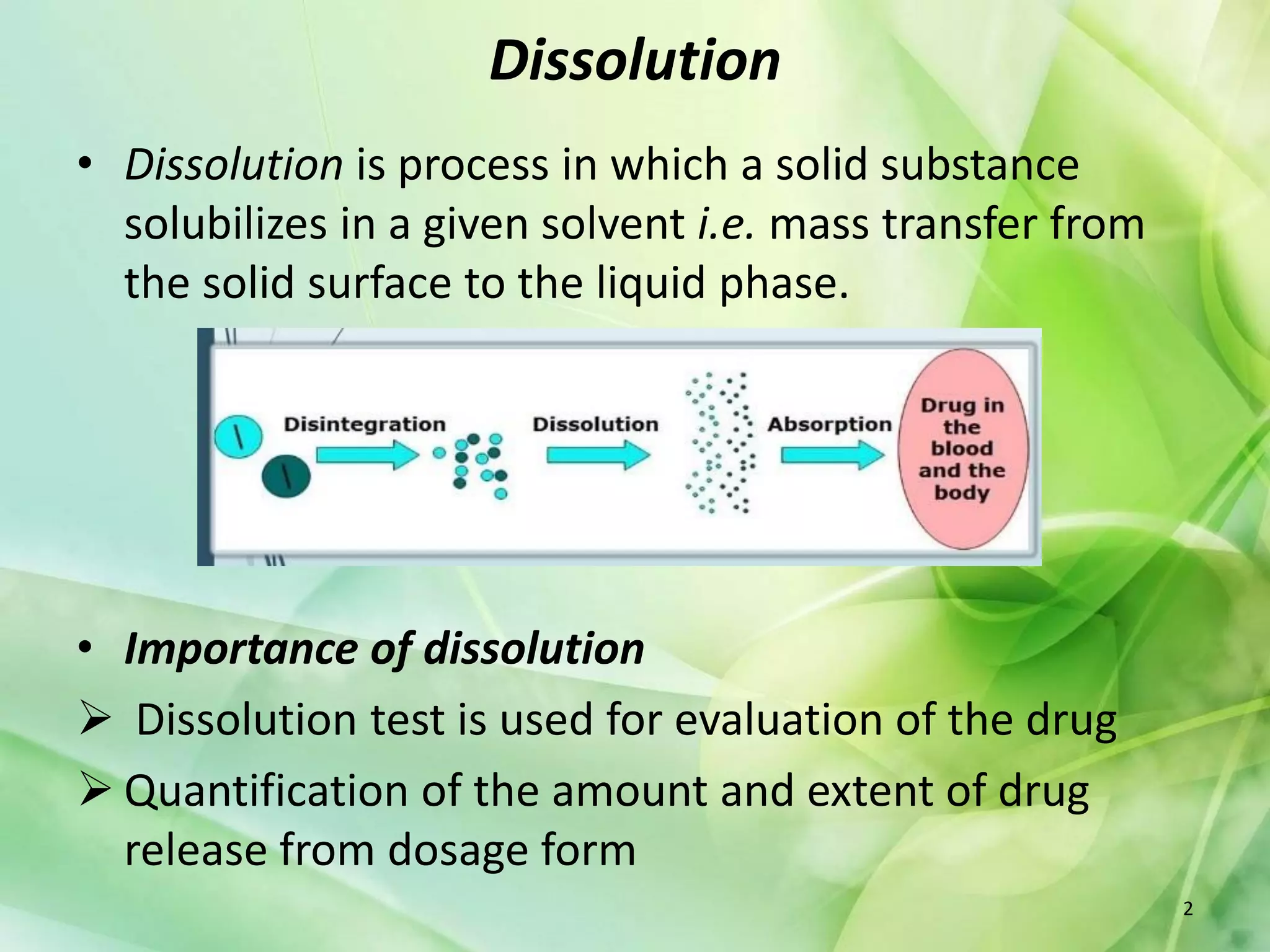
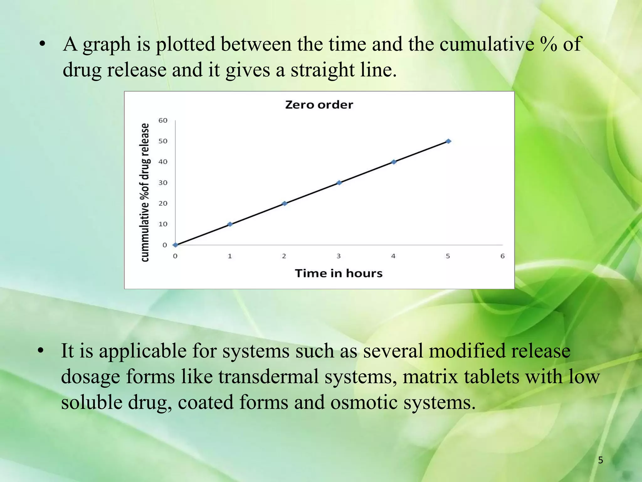
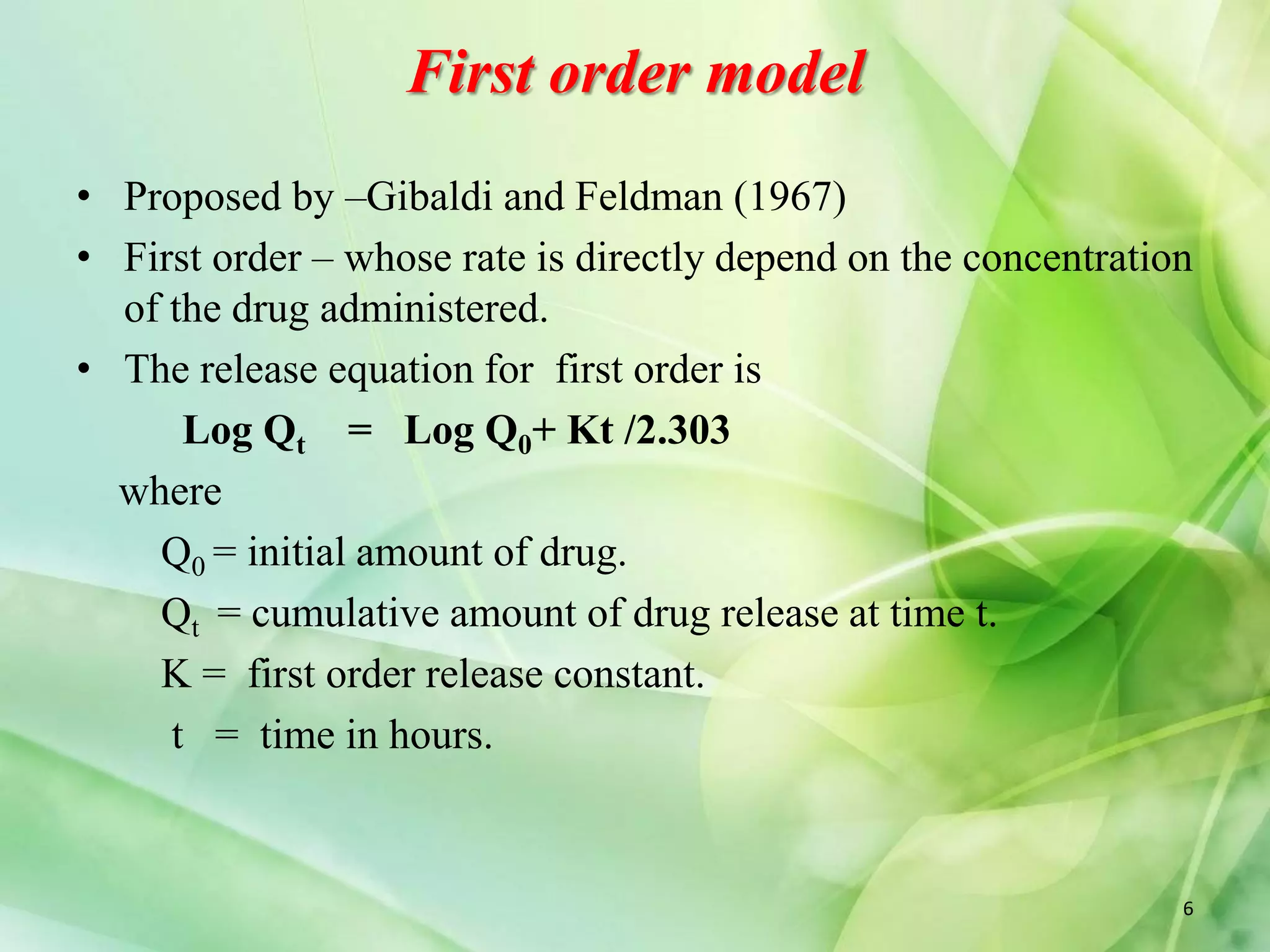
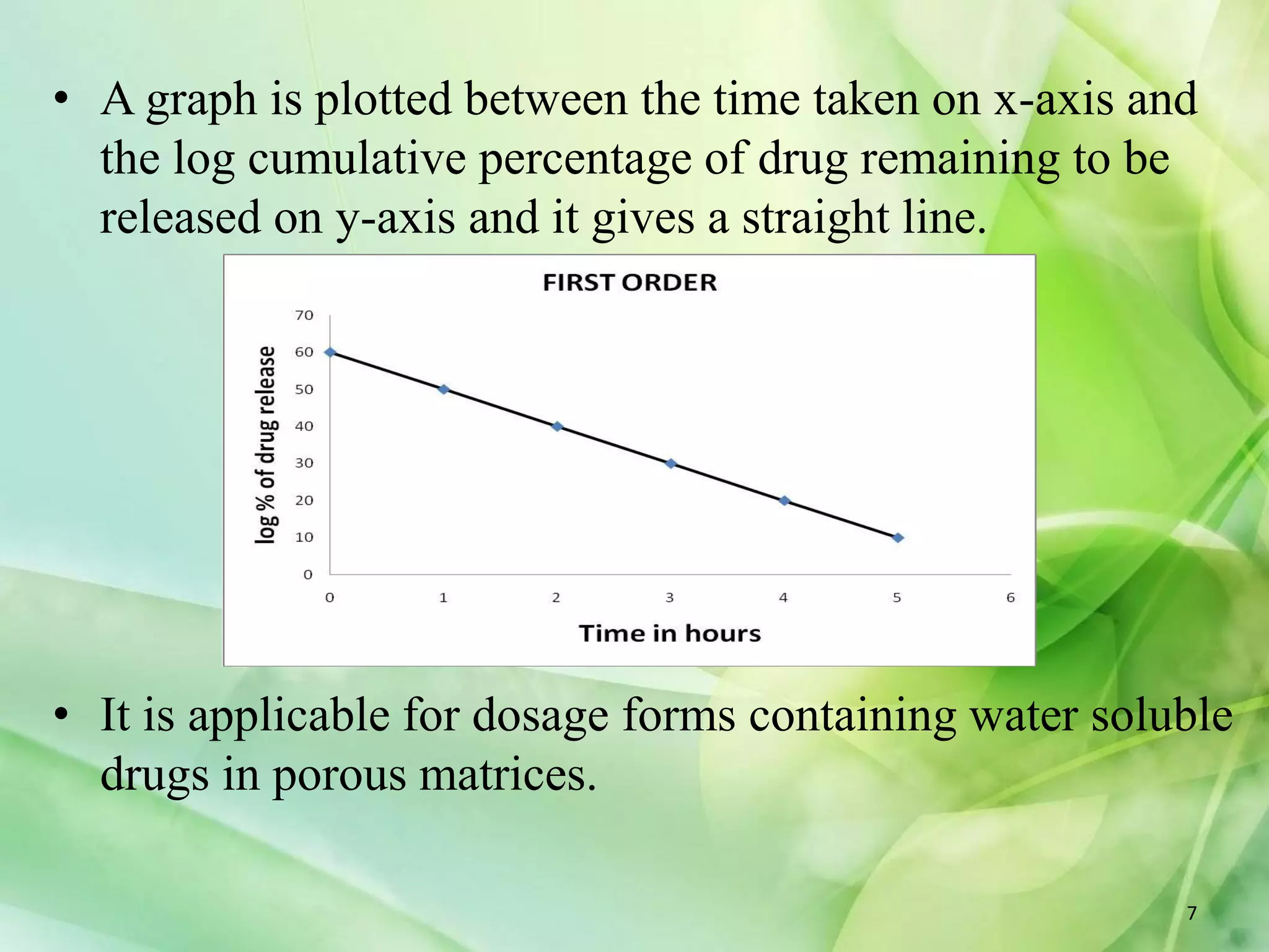
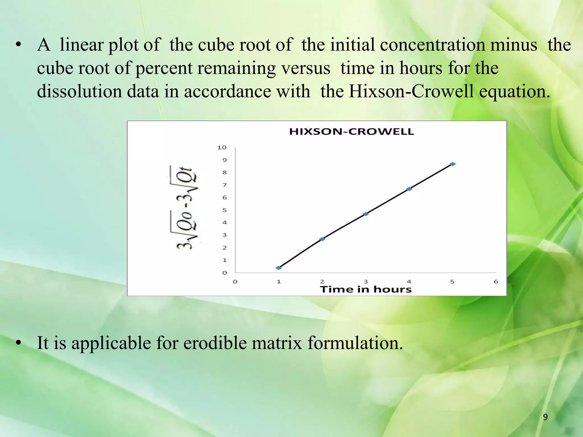
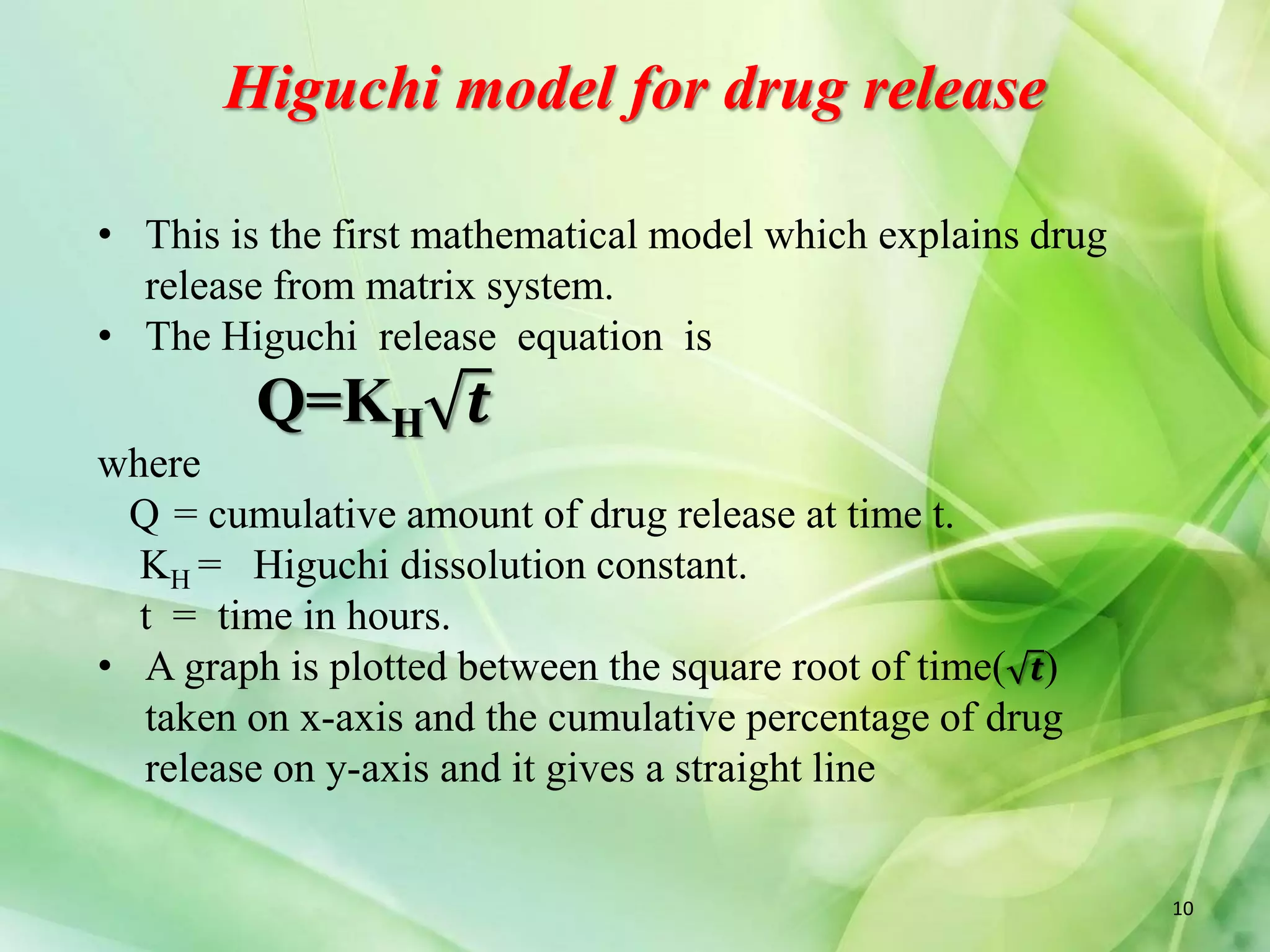
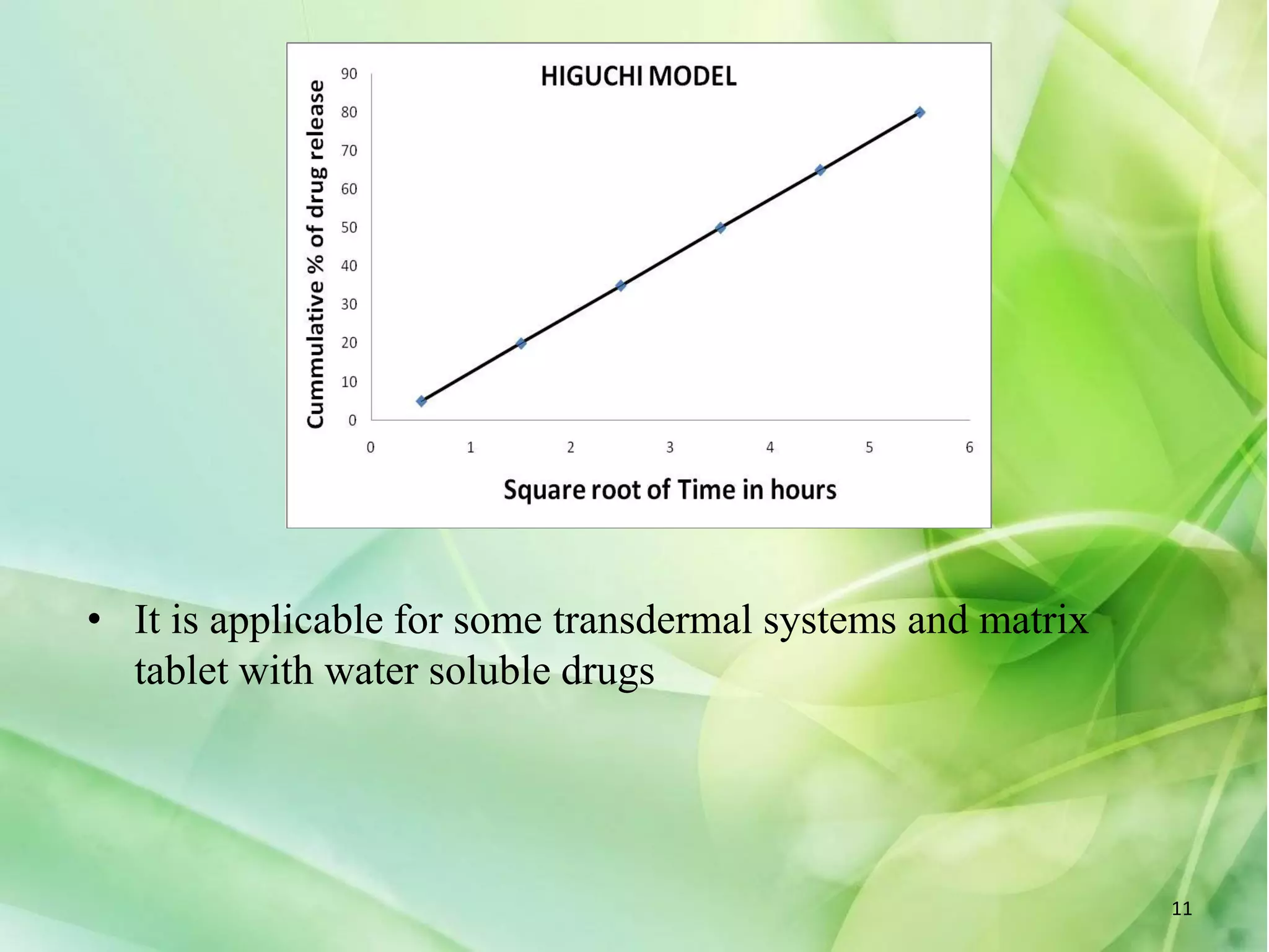
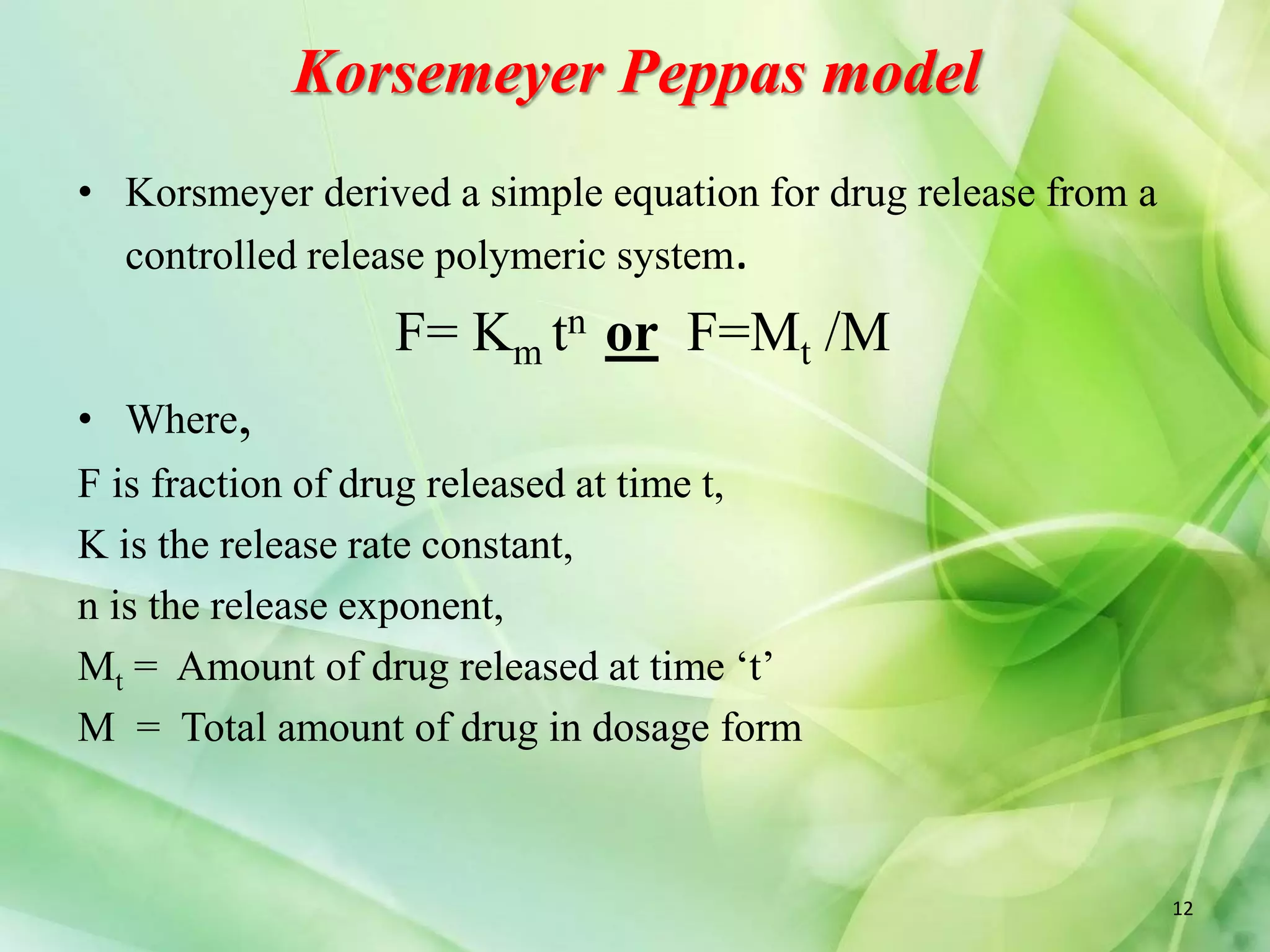
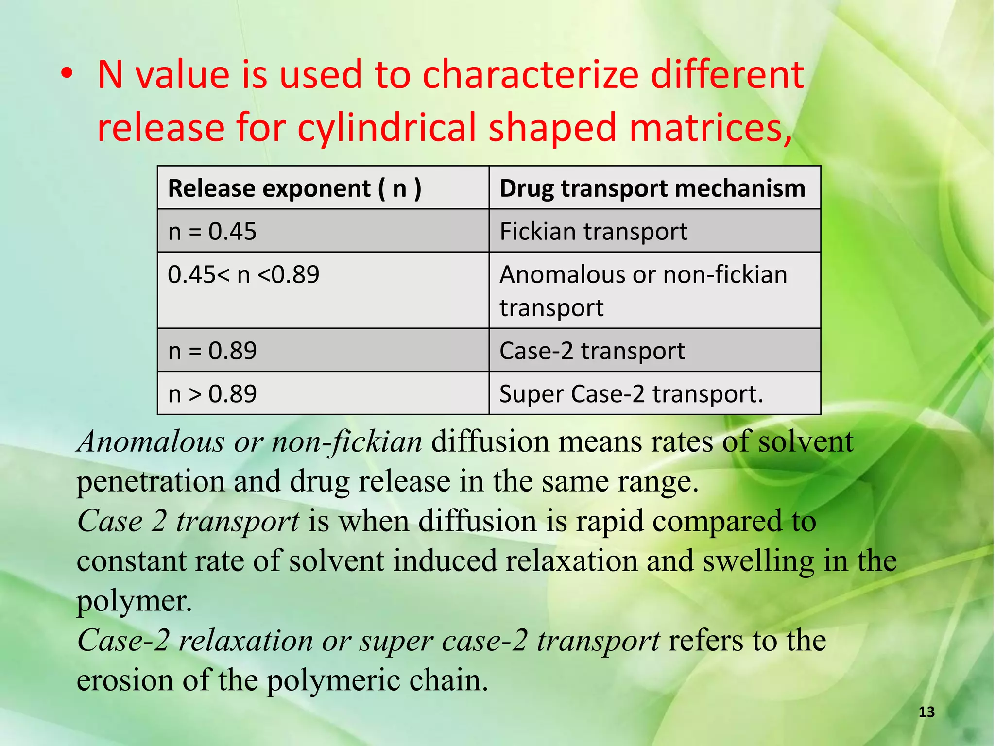
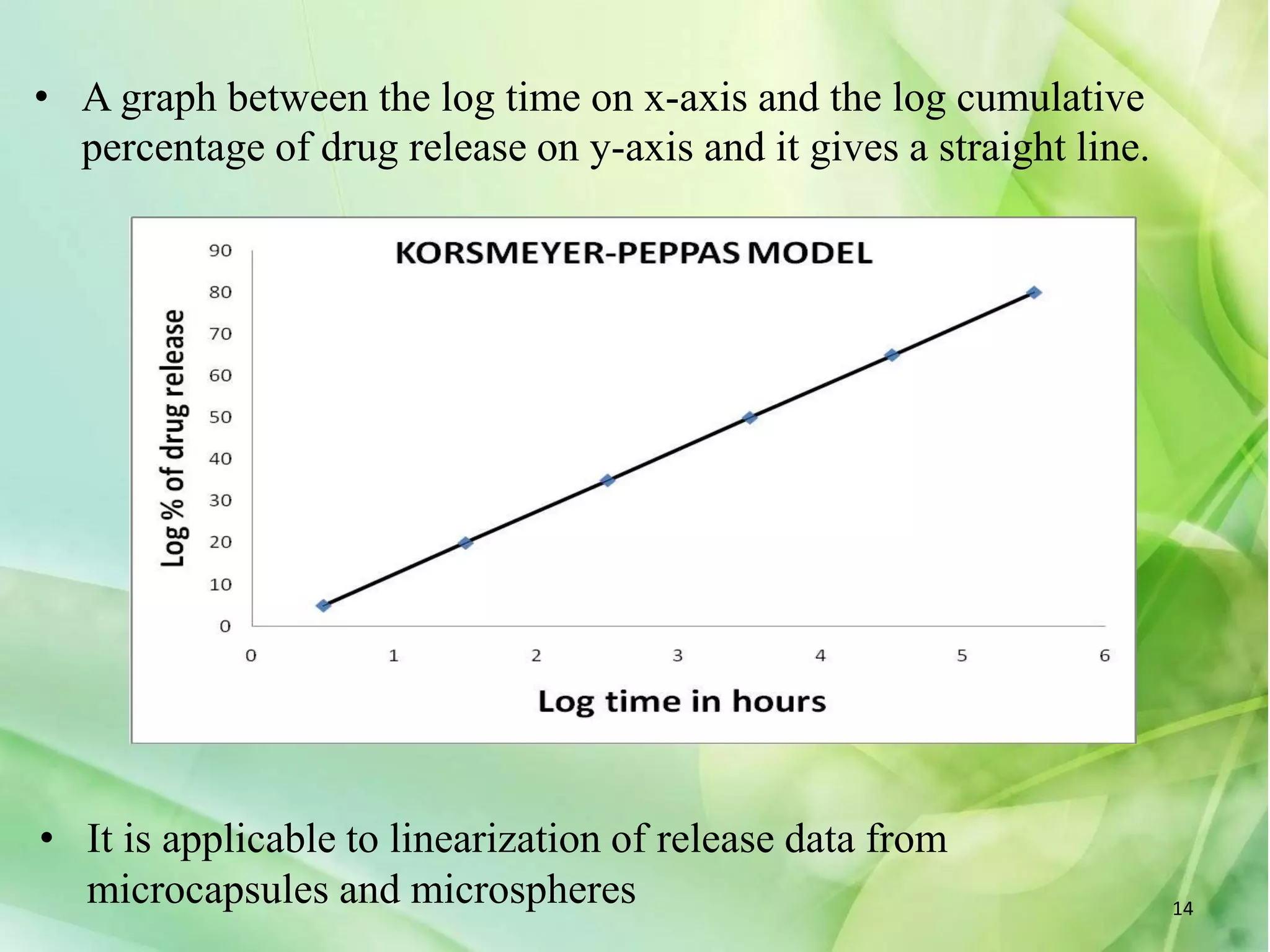
Mathematical models of drug
dissolution
Compiled by
Mr. Aher Sagar Atmaram
M. Pharm 1st Sem.
Department of pharmaceutics.
Guided by
Dr. A.R. Tekade
Head of the Department
Pharmaceutics and QAT.
1
Dissolution
• Dissolution is process in which a solid substance
solubilizes in a given solvent i.e. mass transfer from
the solid surface to the liquid phase.
• Importance of dissolution
 Dissolution test is used for evaluation of the drug
 Quantification of the amount and extent of drug
release from dosage form
2
Mathematical models used to determine
kinetics of drug release
i. Zero order model
ii. First order model
iii.Hixon- and Crowell model
iv.Higuchi model
v. Korsemeyer- peppas model
vi.Weibull model
vii.Baker-lonsdale model
viii.Gompertz model.
3
Zero order model
• The dissolution rate is independent on the concentration of the
drug undergoing reaction.
• Applicable to dosage forms that do not disaggregate and
releases drug slowly
W0 –Wt =Kt……..(1)
Where,
W0 =initial amount of drug dissolved
Wt= amount of the drug in the pharmaceutical
dosage form after time t.
Kt= is the proportionality constant.
4
• A graph is plotted between the time and the cumulative % of
drug release and it gives a straight line.
• It is applicable for systems such as several modified release
dosage forms like transdermal systems, matrix tablets with low
soluble drug, coated forms and osmotic systems.
5
First order model
• Proposed by –Gibaldi and Feldman (1967)
• First order – whose rate is directly depend on the concentration
of the drug administered.
• The release equation for first order is
Log Qt = Log Q0+ Kt /2.303
where
Q0 = initial amount of drug.
Qt = cumulative amount of drug release at time t.
K = first order release constant.
t = time in hours.
6
7
• A graph is plotted between the time taken on x-axis and
the log cumulative percentage of drug remaining to be
released on y-axis and it gives a straight line.
• It is applicable for dosage forms containing water soluble
drugs in porous matrices.
7
Hixon and Crowell model
• Rate of dissolution depends on the surface of the solute, lesser
the surface area greater will be the dissolution
• Hixon and Crowell has derived a equation which expresses
dissolution rate based on the cube root of weight of particles
and radius of the particles is not assumed to be constant.
• Q0
1/3 - Qt
1/3 =kt
• Where
Q0 is the initial amount of drug in dosage form.
Qt is the remaining amount of drug in dosage form at time t.
k is the proportionality constant.
8
• A linear plot of the cube root of the initial concentration minus the
cube root of percent remaining versus time in hours for the
dissolution data in accordance with the Hixson-Crowell equation.
• It is applicable for erodible matrix formulation.
9
Higuchi model for drug release
• This is the first mathematical model which explains drug
release from matrix system.
• The Higuchi release equation is
Q=KH
where
Q = cumulative amount of drug release at time t.
KH = Higuchi dissolution constant.
t = time in hours.
• A graph is plotted between the square root of time( 𝒕)
taken on x-axis and the cumulative percentage of drug
release on y-axis and it gives a straight line
𝒕
10
• It is applicable for some transdermal systems and matrix
tablet with water soluble drugs
11
Korsemeyer Peppas model
• Korsmeyer derived a simple equation for drug release from a
controlled release polymeric system.
F= Km tn or F=Mt /M
• Where,
F is fraction of drug released at time t,
K is the release rate constant,
n is the release exponent,
Mt = Amount of drug released at time ‘t’
M = Total amount of drug in dosage form
12
• N value is used to characterize different
release for cylindrical shaped matrices,
Release exponent ( n ) Drug transport mechanism
n = 0.45 Fickian transport
0.45< n <0.89 Anomalous or non-fickian
transport
n = 0.89 Case-2 transport
n > 0.89 Super Case-2 transport.
Anomalous or non-fickian diffusion means rates of solvent
penetration and drug release in the same range.
Case 2 transport is when diffusion is rapid compared to
constant rate of solvent induced relaxation and swelling in the
polymer.
Case-2 relaxation or super case-2 transport refers to the
erosion of the polymeric chain.
13
• A graph between the log time on x-axis and the log cumulative
percentage of drug release on y-axis and it gives a straight line.
• It is applicable to linearization of release data from
microcapsules and microspheres 14
References
1. Ramteke KH, Dighe PA, Patil SV, mathematical models for
drug dissolution : A review, (SAJP), scholars academic and
scientific publishers, 2014 (3) 5, pg: 388-396.
2. Bramhankar DM, Jaiswal SB, Biopharmaceutics and
pharmacokinetics, Vallabh Prakashan, 2009,pg:431-433.
Thank you
15

Dissolution kinetics and dissolutition modesl

  • 1.
    Mathematical models ofdrug dissolution Compiled by Mr. Aher Sagar Atmaram M. Pharm 1st Sem. Department of pharmaceutics. Guided by Dr. A.R. Tekade Head of the Department Pharmaceutics and QAT. 1
  • 2.
    Dissolution • Dissolution isprocess in which a solid substance solubilizes in a given solvent i.e. mass transfer from the solid surface to the liquid phase. • Importance of dissolution  Dissolution test is used for evaluation of the drug  Quantification of the amount and extent of drug release from dosage form 2
  • 3.
    Mathematical models usedto determine kinetics of drug release i. Zero order model ii. First order model iii.Hixon- and Crowell model iv.Higuchi model v. Korsemeyer- peppas model vi.Weibull model vii.Baker-lonsdale model viii.Gompertz model. 3
  • 4.
    Zero order model •The dissolution rate is independent on the concentration of the drug undergoing reaction. • Applicable to dosage forms that do not disaggregate and releases drug slowly W0 –Wt =Kt……..(1) Where, W0 =initial amount of drug dissolved Wt= amount of the drug in the pharmaceutical dosage form after time t. Kt= is the proportionality constant. 4
  • 5.
    • A graphis plotted between the time and the cumulative % of drug release and it gives a straight line. • It is applicable for systems such as several modified release dosage forms like transdermal systems, matrix tablets with low soluble drug, coated forms and osmotic systems. 5
  • 6.
    First order model •Proposed by –Gibaldi and Feldman (1967) • First order – whose rate is directly depend on the concentration of the drug administered. • The release equation for first order is Log Qt = Log Q0+ Kt /2.303 where Q0 = initial amount of drug. Qt = cumulative amount of drug release at time t. K = first order release constant. t = time in hours. 6
  • 7.
    7 • A graphis plotted between the time taken on x-axis and the log cumulative percentage of drug remaining to be released on y-axis and it gives a straight line. • It is applicable for dosage forms containing water soluble drugs in porous matrices. 7
  • 8.
    Hixon and Crowellmodel • Rate of dissolution depends on the surface of the solute, lesser the surface area greater will be the dissolution • Hixon and Crowell has derived a equation which expresses dissolution rate based on the cube root of weight of particles and radius of the particles is not assumed to be constant. • Q0 1/3 - Qt 1/3 =kt • Where Q0 is the initial amount of drug in dosage form. Qt is the remaining amount of drug in dosage form at time t. k is the proportionality constant. 8
  • 9.
    • A linearplot of the cube root of the initial concentration minus the cube root of percent remaining versus time in hours for the dissolution data in accordance with the Hixson-Crowell equation. • It is applicable for erodible matrix formulation. 9
  • 10.
    Higuchi model fordrug release • This is the first mathematical model which explains drug release from matrix system. • The Higuchi release equation is Q=KH where Q = cumulative amount of drug release at time t. KH = Higuchi dissolution constant. t = time in hours. • A graph is plotted between the square root of time( 𝒕) taken on x-axis and the cumulative percentage of drug release on y-axis and it gives a straight line 𝒕 10
  • 11.
    • It isapplicable for some transdermal systems and matrix tablet with water soluble drugs 11
  • 12.
    Korsemeyer Peppas model •Korsmeyer derived a simple equation for drug release from a controlled release polymeric system. F= Km tn or F=Mt /M • Where, F is fraction of drug released at time t, K is the release rate constant, n is the release exponent, Mt = Amount of drug released at time ‘t’ M = Total amount of drug in dosage form 12
  • 13.
    • N valueis used to characterize different release for cylindrical shaped matrices, Release exponent ( n ) Drug transport mechanism n = 0.45 Fickian transport 0.45< n <0.89 Anomalous or non-fickian transport n = 0.89 Case-2 transport n > 0.89 Super Case-2 transport. Anomalous or non-fickian diffusion means rates of solvent penetration and drug release in the same range. Case 2 transport is when diffusion is rapid compared to constant rate of solvent induced relaxation and swelling in the polymer. Case-2 relaxation or super case-2 transport refers to the erosion of the polymeric chain. 13
  • 14.
    • A graphbetween the log time on x-axis and the log cumulative percentage of drug release on y-axis and it gives a straight line. • It is applicable to linearization of release data from microcapsules and microspheres 14
  • 15.
    References 1. Ramteke KH,Dighe PA, Patil SV, mathematical models for drug dissolution : A review, (SAJP), scholars academic and scientific publishers, 2014 (3) 5, pg: 388-396. 2. Bramhankar DM, Jaiswal SB, Biopharmaceutics and pharmacokinetics, Vallabh Prakashan, 2009,pg:431-433. Thank you 15