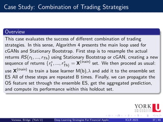
This document summarizes a presentation about using generative adversarial networks (GANs) and ensemble modeling for financial applications. It discusses how GANs can generate synthetic financial time series data to augment training datasets and test trading strategies. The presentation covers GAN and conditional GAN architectures, model training procedures, and experiments evaluating trading strategy performance on synthetic versus real data. It finds that ensembling multiple strategies trained on synthetic data outperforms individual strategies, demonstrating the value of GANs and ensemble modeling for financial applications.
![Why Use These Techniques?
(i) Generate more diverse training and testing sets, compared to traditional
resampling techniques;
(ii) Provides the ability to draw samples specifically about stressful events,
ideal for model checking and stress testing; and
(iii) Provides a level of anonymization to the dataset, differently from
other techniques that (re)shuffle/resample data.[1]
Vanessa, Bridge (York U) Deep Learning Strategies For Financial Applications ICLR 2023 4 / 49](https://image.slidesharecdn.com/seminar2deeplearningapplicationsinfinance-230919030515-a8073a03/85/Deep-Learning-Applications-in-Finance-pdf-4-320.jpg)
![Conditional GAN
A Conditional GAN (cGAN) attempts to learn an implicit conditional
generative model by using extra input data V:
a class label,
a certain categorical feature,
a current/expected market condition
It is specially useful when the data follows a sequence, like time series or
text, or wants to build ”what if” scenarios.
Defintion
Formally a cGAN can be defined by including the conditional variable v:
G : z × v −
→ x and D : x∗ × v −
→ [0, 1]
D and G follow a two-player minmax game with value function V (G, D) :
minG maxD V (D, G) = Ex pdata(x)
[logD(x|v)]+Ez pdata(z)
[log(1−D(G(z|v)))]
Vanessa, Bridge (York U) Deep Learning Strategies For Financial Applications ICLR 2023 16 / 49](https://image.slidesharecdn.com/seminar2deeplearningapplicationsinfinance-230919030515-a8073a03/85/Deep-Learning-Applications-in-Finance-pdf-16-320.jpg)
![Model Training: Stochastic Gradient (SG)
Much like regular GANs, training cGANs consists of a similar approach
using a Stochastic Gradient minibatch. The SG is calculated using L
samples from the mini batch and z is the noise vector.
Stochastic Gradient Discriminator
∇θD
1
L
PL
l=1[logD(y
(l)
t |y
(l)
t−1, ..., y
(l)
t−p) + log(1 − D(G(z(l)|y
(l)
t−1, ..., y
(l)
t−p)]
Stochastic Gradient Generator
∇θG
1
L
PL
l=1[logD(G(z(l)|y
(l)
t−1, ..., y
(l)
t−p))]
However selecting the rigth cGAN can be a difficult task that is
computationally expensive and so using snapshots as a way to evaluate
them at different points in time should be considered.
Vanessa, Bridge (York U) Deep Learning Strategies For Financial Applications ICLR 2023 21 / 49](https://image.slidesharecdn.com/seminar2deeplearningapplicationsinfinance-230919030515-a8073a03/85/Deep-Learning-Applications-in-Finance-pdf-21-320.jpg)
![Model Validation: Data Selection
Finite set of examples: X(train), draw from a probability distribution
px (x)
Set of hyperparameters λ ∈ Λ, such as number of neurons, activation
function of layer j, etc.
Utility function P to measure a trading strategy Sλ performance in
face of new samples from px (x)
trading strategy Mλ with parameters θ identifiable by an optimization
of a training criterion, but only spotted after a certain λ is fixed
Optimal Configuration
λ∗ = arg max{λ∈Λ} Ex px [P(x; Mλ(Xtrain
))]
Vanessa, Bridge (York U) Deep Learning Strategies For Financial Applications ICLR 2023 24 / 49](https://image.slidesharecdn.com/seminar2deeplearningapplicationsinfinance-230919030515-a8073a03/85/Deep-Learning-Applications-in-Finance-pdf-24-320.jpg)
![Hyperparameter Optimization And Model Validation
Optimal vs. Approximation
Challenges arise when trying to use the previous formula due to the
difficulty in generating new samples from px (x). Additionally Λ can be
extremely large.
Approximation
λ∗ = arg max{λ∈Λ} Ex px [P(x; Mλ(Xtrain
))]
≈ arg max{λ∈{λ1,λ2,...,λm} Ex px [P(x; Mλ(Xtrain
))]
≈ arg max{λ∈{λ1,λ2,...,λn} meanx∈X(val) [P(x; Mλ(Xtrain
))]
Vanessa, Bridge (York U) Deep Learning Strategies For Financial Applications ICLR 2023 25 / 49](https://image.slidesharecdn.com/seminar2deeplearningapplicationsinfinance-230919030515-a8073a03/85/Deep-Learning-Applications-in-Finance-pdf-25-320.jpg)
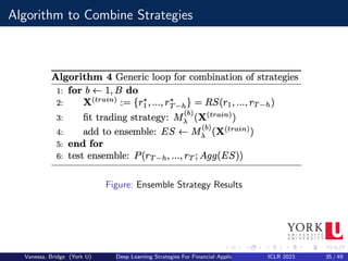
![Sampling And Aggregation
Ensemble Of Trading Strategies
By combining a set of base learners, usually considered ”Weak”, such as
Classification and Regression Tree, aggregation of these strategies can out
compete ”strong” learners such as SVM. These method can be compared
to bagging.
Variance Reduction
Let Y1, ..., YB be a set of base learners. If we average their predictions and
analyse its variance we get:
V[ 1
B
PB
b=1 Ŷb] = 1
B2 (
PB
b=1 V[Ŷb] + 2
PB
1≤b≤j≤B C[Ŷb, Ŷj ])
if we assume V[Ŷb] = σ2 and C[Ŷb, Ŷj ] = ρσ2 that simplifies to:
V[ 1
B
PB
b=1 Ŷb] = σ2( 1
B + B−1
B ρ) ≤ σ2
Vanessa, Bridge (York U) Deep Learning Strategies For Financial Applications ICLR 2023 28 / 49](https://image.slidesharecdn.com/seminar2deeplearningapplicationsinfinance-230919030515-a8073a03/85/Deep-Learning-Applications-in-Finance-pdf-28-320.jpg)
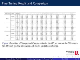
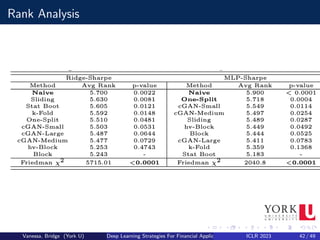
![Fine-Tuning Results
Results
We can spot that there not much differences between the model validation
schemes, with Naive yielding the worst median (50%) values (0.121), and
hv-Block, Block and cGAN-Medium with the best median (0.138); same
can be said with respect to Calmar ratios.
Overall, apart from a few analyses and cases (e.g., GBT and Naive
method), in aggregate the model validation schemes do not appear to be
significantly distinct from each other.
This can be interpreted that cGAN is a viable procedure to be part of the
fine-tuning pipeline, since its results are statistically indistinguishable to
well established methodologies[1].
Vanessa, Bridge (York U) Deep Learning Strategies For Financial Applications ICLR 2023 41 / 49](https://image.slidesharecdn.com/seminar2deeplearningapplicationsinfinance-230919030515-a8073a03/85/Deep-Learning-Applications-in-Finance-pdf-41-320.jpg)
![Applications to cGAN
Another interesting application is to use cGANs for medical time series
generation and anonymization. A group of researchers used cGANs to
generate realistic synthetic medical data, so that this data could be shared
and published without privacy concerns, or even used to augment or enrich
similar datasets collected in different or smaller cohorts of patients.
Most of the applications of cGANs related to the work presented have
centred in synthesizing data to improve supervised learning models. The
only exception is, where a cGAN is used to perform direction prediction in
stock markets[2].
Most work deals with the problem of imbalanced classification, in
particular to fraud detection; it has been shown that cGANs compare
favourably to other traditional techniques for oversampling.
Vanessa, Bridge (York U) Deep Learning Strategies For Financial Applications ICLR 2023 46 / 49](https://image.slidesharecdn.com/seminar2deeplearningapplicationsinfinance-230919030515-a8073a03/85/Deep-Learning-Applications-in-Finance-pdf-46-320.jpg)
![Challenges
Is the GAN memorising the training data?
Is the GAN ignoring data samples it cannot reproduce or over
producing the ones it can easily reproduce (i.e.: mode collapse) [3]
Potential risk that cGAN is unable to replicate well pdata and
although samples might be more diverse they are also more ”biased”
Vanessa, Bridge (York U) Deep Learning Strategies For Financial Applications ICLR 2023 47 / 49](https://image.slidesharecdn.com/seminar2deeplearningapplicationsinfinance-230919030515-a8073a03/85/Deep-Learning-Applications-in-Finance-pdf-47-320.jpg)
![Conclusion
Over these presentation were able to demonstrate the relevance of having
a set of model assessment schemes, using cGAN to identify alpha
opportunities that other techniques are unable to find. Furtheremore, the
research shows that it is possible to generate more diverse training and
testing sets, compared to traditional resampling techniques[1].
The findings encourage the further investigation of cGAN techniques for
other applications not covered here such as stress testing. We also need to
keep in mind the current limitations and to consider further exploration of
the techniques by combining with other methods[4].
Vanessa, Bridge (York U) Deep Learning Strategies For Financial Applications ICLR 2023 48 / 49](https://image.slidesharecdn.com/seminar2deeplearningapplicationsinfinance-230919030515-a8073a03/85/Deep-Learning-Applications-in-Finance-pdf-48-320.jpg)