Database

1. The Relational Data Model, Relational
Database Constraints and Relational
Algebra
Unit 3

2. Chapter 5:
Outline
 Relational Model Concepts
 Relational Model Constraints
 Relational Database Schemas
 Update Operations, Transactions and Dealing
with Constraint Violations

3.  The relational data model was first introduced by
Ted Codd of IBM Research in 1970
 The first commercial implementations of the
relational model became available in the early
1980s – IBM, Oracle DBMS.
 Current popular relational DBMSs (RDBMSs)
include:
 DB2 and Informix Dynamic Server (from IBM),
 Oracle and Rdb (from Oracle),
 Sybase DBMS (from Sybase / SAP)
 SQLServer and MS Access (from Microsoft).
 Open source systems – MySQL, PostgreSQL

4. Relational Model Concepts
 The relational Model represents the db as a
collection of Relations.
 Each relation resembles a table of values.
 A row in a table represents a collections of
related data values.
 A table name & column names are used to help
to interpret the meaning of the values in each
row.
 Ex: Student table

5.  This table is called STUDENT because each row
represents facts about a particular student entity.
 The column names Name, Stu_no, etc specify
how to interpret the data values in each row,
based on the column values in.
 All values in a column are of the same data type.

6. Fig 5.1: The attributes and tuples of a relation STUDENT

7.  A row is called a tuple
 A column header is called an attribute
 The table is called a relation
 The data type describing the types of values that
can appear in each column is represented by a
domain of possible values.
In the formal relational model terminology:

8. Domains:
 A domain D is a set of atomic values.
 Means that each value in the domain is
indivisible as far as the relational model is
concerned.
 Ex: phone_numbers - set of 10 digit phone
numbers.
 A domain may have a data-type or a format
defined for it.
 The phone_numbers may have a format: ddd-
ddddddd where each d is a decimal digit.
 Dates have various formats such as month name,
date, year or yyyy-mm-dd, or dd-mm-yyyy etc.

9. Informal Terms Formal Terms
Table Relation
Column Attribute/Domain
Row Tuple
Values in a column Domain
Table Definition Schema of a Relation
Populated Table Extension

10. Relation schema (R)
 Is used to describe a relation.
 A relation schema R denoted by R(A1,A2,…An).
 Is made up of relation name R and a list of
attributes A1,A2,…An.
 Each attribute Ai is the name of a role played by
some domain D in the relation schema R.
 D is called domain of Ai and is denoted by
dom(Ai).

11. Degree of a relation:
 Is the number of attributes n of its relation.
Ex: STUDENT( Name, Address, Age, phone)
Degree of a relation STUDENT is 4
 Using the data type of each attribute, the
definition is sometimes written as:
STUDENT( Name : string, Address : string,
Age : integer, phone : string)

12. Relation state:
 A relation (or relation state) r of the relation
schema R(A1, A2,….., An) is a set of n-tuples
r = { t1, t2, …., tm }.
 Each n-tuple t is an ordered list of n values
t = < v1, v2, … vn >, where each value vi, 1≤ i ≤ n
is an element of dom(Ai) or is a special NULL
value.
 ith
value in tuple t, which corresponds to the
attribute Ai, is reffered to as t[Ai].
 Relation state is denoted as r(R).

13. FORMAL DEFINITION:
 A relation (or relation state) r(R) is a
mathematical relation of degree n on the
domains dom(A1), dom(A2),…. dom (An), which
is a subset of the Cartesian product of the
domains that define R:
r(R)  dom (A1) X dom (A2) X ....X dom(An)
 The Cartesian product specifies all possible
combinations of values from the underlying
domains.
 Terms: relation intension - schema R
relation extension - relation state
r(R)

14.  Current relation state: a relation state at a
given time.
- Reflects only the valid tuples that represent a
particular state of the real world.
- Relation state – Relatively dynamic
- Schema R – relatively static and does not
change except very infrequently
ex: adding a new attribute.

15.  Ordering of tuples in a relation r(R): Tuples in
a Relation do not have any particular order even
though they appear to be in the tabular form.
 Tuple ordering is not part of a relation definition
because a relation attempts to represent facts
at a logical or abstract level
 The definition of a relation does not specify any
order.
 Many logical orders can be specified on a
relation. Ex: fig: 5.2
 When we display a relation as a table, the rows
are displayed in a certain order.
CHARACTERISTICS OF RELATIONS

16. Fig 5.2: The attributes and tuples of a relation STUDENT

17.  Ordering of Values within a tuple and an alternative
Definition of a Relation :
 At a logical level, the order of attributes and their values
is not that important as long as the correspondence
between attributes and values is maintained.
Alternative Definition:
- A relation schema R= {A1, A2, ..., An } is a set of attributes
- A relation state r(R) is a finite set of mappings r = { t1,
t2,…, tm}, where each tuple ti is a mapping from R
to D., and D is the union of the attribute domains; that
is
D = dom (A1) U dom (A2) U …. U dom (An)
- In this definition, t[Ai] must be in dom(Ai) for 1≤ i ≤ n for
each mapping t in r.
- Each mapping ti is called a tuple.

18.  Values and NULLs in the tuple:
 All values are considered atomic (indivisible).
 Hence, composite and multivalued attributes are not
allowed.
 Relational model is based on 1NF
 A special null value is used to represent values that
are unknown or inapplicable to certain tuples.
 Ex:

19. Interpretation (Meaning) of a Relation.
 The relation schema can be interpreted as a
declaration or a type of assertion.
 Ex: The schema of the STUDENT relation of
Figure 3.1 asserts that, in general, a student
entity has a Name, Ssn,Home_phone, Address,
Office_phone, Age, and Gpa.
 Each tuple in the relation can then be interpreted
as a fact or a particular instance of the
assertion. Ex: the first tuple in Figure 3.1 asserts
the fact that there is a STUDENT whose Name
is Benjamin Bayer, Ssn is 305-61-2435, Age is
19, and so on.

20.  Notice that some relations may represent facts
about entities, whereas other relations may
represent facts about relationships.
 The relational model represents facts about both
entities and relationships uniformly as relations.
 In Entity-Relationship (ER) model the entity and
relationship concepts will be described in detail.
 An alternative interpretation of a relation schema
is as a predicate; in this case, the values in
each tuple are interpreted as values that satisfy
the predicate.

21.  For example, the predicate STUDENT (Name,
Ssn, ...) is true for the five tuples in relation
STUDENT of Figure 3.1.
 These tuples represent five different propositions
or facts in the real world.
 This interpretation is quite useful in the context of
logical programming languages, such as Prolog,
because it allows the relational model to be used
within these languages

22. Relational model notation
 A relation schema R of degree n is denotes by R
(A1, A2,…, An)
 The letters Q,R,S denote relation names.
 The letters q,r,s denote relation states.
 The letters t,u,v denote tuples.
 In general, the name of a relation schema such
as STUDENT also indicate the current set of
tuples in the relation – the current relation state-
whereas STUDENT (Name, Ssn,….) refers only
to the relation schema.

23.  An attribute A can be qualified with the relation
name R to which it belongs by using the dot
notation R.A
 Ex: STUDENT.Name, STUDENT.Age
Because the same name may be used for two
attributes in different relations.
 We refer to component values of a tuple t by
t[Ai] and t.Ai = vi (the value of attribute Ai for tuple
t).

24. Relational Model Constraints & Relational
Database Schemas
 Constraints on dbs can be generally be divided
into three main categories:
1.Inherent model-based or implicit constraints:
Constraints that are inherent in the data model.
ex: relation cannot have duplicate tuple.
2. Schema-based or explicit constraints:
Constraint that can be directly expressed in
schemas of the data model, typically by specifying
them in the DDL.

25. 3. Application-based or semantic constraints or
business rule:
Constraint that cannot be directly expressed in
schemas of the data model, & hence must be
expressed & enforced by the application
programs.
This constraint checked within application
programs.
4. Data dependencies – Functional dependency
Multivalued
dependency
Used mainly for testing the goodness of a
relational db.
Utilized in the Normalization process.

26. Domain Constraints
 Specify that within each tuple, the value of each
attribute A must be an atomic value from the
domain dom(A).
 The data types associated with domains typically
include standard data types:ex:
 Integers – int, short int, long int etc.,
 Real numbers – float, double, precision float etc.,
 Characters, Booleans, fixed-length strings,
variable-length strings are also available
 Special data types – date, time, time-stamp, money

27. Relational Integrity Constraints
 Constraints are conditions that must hold on
all valid relation instances. There are three
main types of constraints:
 Key constraints
 Entity integrity constraints
 Referential integrity constraints

28. Key Constraints and Constraints on NULL values
 Superkey of R: Is a set of one or more
attributes that allow us to identify uniquely a
tuple in the relation.
- Specifies uniqueness
 That is, for any distinct tuples t1 and t2 in r(R),
t1[SK]  t2[SK].
ex: Emp-id in Employee relation.
Superkey: An attribute, or group of attributes, that is
sufficient to distinguish every tuple in the relation from
every other one.

29. Candidate key:
- Each super key is called a candidate key
- A candidate key is all those set of attributes which
can uniquely identify a row.
- However, any subset of these set of attributes
would not identify a row uniquely
Ex: In shipment table, “S# , P# ” is a candidate key.
But, S# alone or P# alone would not uniquely
identify a row of the shipment table.
Note: Every super key cannot be a candidate key,
where as all candidate keys are super keys

30.  Simple candidate key:
A candidate key comprising of one attribute only.
ex: Acc_no, Cust_id, Cust_email etc.,
 Composite candidate key:
A candidate key comprising of two or more
attributes.
Ex: { Cust_last_name, Cust_first_name}
One attribute is not enough

31.  Invalid candidate key:
- A candidate key should be comprised of a set
of attributes that can uniquely identify a row.
- A subset of the attributes should not posses the
unique identification property.
Ex: the combination of { acc_no, Acc_type}
Here acc_no alone is a candidate key.
 Candidate key are identified during the design of
the db.

32.  Primary key
One of the candidate key whose value is used to
uniquely identify the tuples in the relation.
Ex: Acc_no, Empno etc.,
Conventions:
- the attribute that form the primary key of a relation
schema are underlined.
- It is preferable to choose a primary key with a single
attribute or a small number of attributes.
- Give preference to numeric column(s)
- PKs are chosen according to business convenience.
 A primary key which is a combination of more than
one attribute is called a composite primary key

33.  Non-key attributes:
The attributes other than the primary key
attributes in a relation are called non-key
attributes.
ex: Emp – Ename, Salary, dept, etc.,
 Constraints on NULL values:
Another constraint on attributes specifies
whether NULL values or not permitted.
Ex: NOT NULL constraint.

34. Relational Database and Relational Database schema
 A relational database schema S is a set of
relation schemas S = { R1, R2,….,Rm } & set of
integrity constraints IC.
 A relational database state DB of S is a set of
relation states DB={r1, r2, …, rm} such that each ri
is a state of Ri and such that the ri relation states
satisfy the integrity constraints specified in IC.

37.  A db state that does not obey all the IC is called
an invalid state, and a state that satisfies all
the constraint in IC is called an valid state.
 Each relational DBMS must have a data
definition language (DDL) for defining a
relational db schema.
 Current relational DBMSs are using SQL.
 IC are specified on a db schema and are
expected to hold on every valid db state of that
schema.

38. Entity Integrity
 States that no primary key value can be NULL.
Key constraints and Entity constraints are specified on
individual relations.
Referential Integrity Constraint
- Is specified between two relations and is used to
maintain the consistency among tuples in the two
relations.
- Informally RIC states that a tuple in one relation that
refers to another relation must refer to an existing
tuple in that relation.
- Ex: Dno of Emp and Dnum of Dept

39. Foreign key
 A set of attributes FK in relation schema R1 is a foreign
key of R1 that references relation R2 if it satisfies the
following rules:
 The Attributes in FK have the same domain(s) as the
PK attributes of R2; the attributes FK are said to
reference or refer to the relation R2.
 A value of FK in tuple ti of the current state r1(R1)
either occurs as a value of PK for some tuple t2 in the
current state r2(R2) or is null.
i.e. t1[FK] = t2[PK] and we say that the tuple t1
references or refer to the tuple t2.

40.  In this definition, R1 – referencing relation
R2 – referenced relation
 If these two conditions hold, a RIC from R1 to
R2 is said to hold.
 In a db of many relations, there are usually
many RIC.
 Foreign key values do not (usually) have to be
unique
 Foreign keys can also be null
 Foreign key can refer to its own relation. (Self
referenced relation)

43. Other types of constraints:
 Semantic integrity constraints: Specified and
enforced on a relational db. Ex: Sal of emp
should not exceed the sal of his Supervisor.
Mechanisms: Triggers, Assertions.
 Functional Dependency: X determines Y
 State constraints: Constrains that a valid db
must satisfy.
 Transaction constraints: Defined to deal with
state changes in the db.
 - enforced by Application pgms, Triggers,…

44. Update operations, Transactions, and dealing
with Constraint Violations
The operations of the Relational Model
categorized into:
 Retrievals
 Updates
Concentrating on Database modification or
update operations

45.  Three basic update operations on relations:
 Insert - new data – insert new tuple(s)
 Delete - old data – delete tuples
 Modify – existing data – change the values of some
attributes.
 Integrity constraints should not be violated by
any of these operations.
 Discussion on types of constraints violated by
the update operation and the types of actions
that may be taken in case violation.

46. The Insert operation
 Provides a list of attribute values for a new tuple
t that is to be inserted into a relation R.
 Can violate : Domain Constraint
Key constraint
Entity Integrity Constraint
Referential Integrity Constraint
Domain Constraint : violated if an attribute
value is given that does not appear in the
corresponding domain.

47. Key constraint: violated if a key value in the new
tuple t already exists in another tuple in the
relation r(R)
Entity integrity : violated if the primary key of the
new tuple t is NULL.
Referential Integrity: violated if the value of any
foreign key in t refers to a tuple that does not
exist in the referenced relation.

48.  Insert <‘Cecilia’, ‘F’, ‘Kolonsky’, NULL, ‘1960-04-05’,
‘6357 Windy Lane, Katy,TX’, F, 28000, NULL, 4>
into EMPLOYEE.
Result: This insertion violates the entity integrity
constraint (NULL for the primary key Ssn), so it is
rejected.

49.  Insert <‘Alicia’, ‘J’, ‘Zelaya’, ‘999887777’, ‘1960-04-
05’, ‘6357 Windy Lane, Katy,TX’, F, 28000,
‘987654321’, 4> into EMPLOYEE.
Result: This insertion violates the key constraint
because another tuple with the same Ssn value
already exists in the EMPLOYEE relation, and so it is
rejected.

50.  Insert <‘Cecilia’, ‘F’, ‘Kolonsky’, ‘677678989’, ‘1960-04-
05’, ‘6357 Windswept, Katy, TX’, F, 28000, ‘987654321’,
7> into EMPLOYEE.
Result: This insertion violates the referential integrity
constraint specified on Dno in EMPLOYEE because no
corresponding referenced tuple exists in DEPARTMENT
with Dnumber = 7.

51.  Insert <‘Cecilia’, ‘F’, ‘Kolonsky’, ‘677678989’,
‘1960-04-05’, ‘6357 Windy Lane, Katy, TX’, F,
28000, NULL, 4> into EMPLOYEE.
 Result: This insertion satisfies all constraints, so
it is acceptable.

52. In case of constraints violation, several actions
can be taken:
 Default option – reject the insertion
 Explain the user why the insertion was rejected.
 Attempt to correct the reason for rejecting the
insertion.
 Execute a user-specified error-correction routine

54. The Delete Operation
 Can violate only referential integrity.
 If the tuple being deleted is referenced by the
foreign keys from other tuples in the db.
 Ex:
 Delete the WORKS_ON tuple with Essn =
‘999887777’ and Pno = 10.
 Result: This deletion is acceptable and deletes
exactly one tuple.

55.  Delete the EMPLOYEE tuple with Ssn =
‘999887777’.
 Result: This deletion is not acceptable,
because there are tuples in WORKS_ON that
refer to this tuple. Hence, if the tuple in
EMPLOYEE is deleted, referential integrity
violations will result.
 Delete the EMPLOYEE tuple with Ssn =
‘333445555’.

56. In case of constraints violation,
options:
• Reject the deletion
• Attempt to cascade the deletion
• Modify the referencing attribute values

57. The Update Operation
 The update (or Modify) operation is used to
change the values of one or more attributes in a
tuple (or tuples) of some relation R.
 It is necessary to specify the condition on the
attributes of the relation to select the tuple (or
tuples) to be modified.

58.  Update the salary of the EMPLOYEE tuple with Ssn =
‘999887777’ to 28000.
 Result: Acceptable.
 Update the Dno of the EMPLOYEE tuple with Ssn =
‘999887777’ to 1.
 Result: Acceptable.

59.  Update the Dno of the EMPLOYEE tuple with Ssn =
‘999887777’ to 7.
 Result: Unacceptable, because it violates referential
integrity.
 Update the Ssn of the EMPLOYEE tuple with Ssn =
‘999887777’ to ‘987654321’.
 Result: Unacceptable, because it violates primary key
constraint

60. The Transaction Concept
 A db application program running against a
relational db typically runs a series of
transaction.
 A transaction involves:
 Reading from the db
 Doing insertion, deletions, and updates to
exsiting values in the db.
 Transaction must leave the db in a consistent
state; State that obey all the constraints.
 A single transaction may involve any number of
retrieval operations and update operations.

61. Chapter 8: The Relational Algebra and
Relational Calculus
 Historically, the relational algebra and calculus
were developed before the SQL language.
 In fact, in some ways, SQL is based on concepts
from both the algebra and the calculus
 Because most relational DBMSs use SQL as
their language, we presented the SQL language
first.

62.  The basic set of operations for the relational
model is the relational algebra.
 These operations enable a user to specify basic
retrieval requests as relational algebra
expressions.
 The result of a retrieval is a new relation, which
may have been formed from one or more
relations.
 A sequence of relational algebra operations
forms a relational algebra expression, whose
result will also be a relation that represents the
result of a database query (or retrieval request).

63. Importance of relational algebra
 First, it provides a formal foundation for
relational model operations.
 Second – Important - it is used as a basis for
implementing and optimizing queries in the
query processing and optimization modules that
are integral parts of relational database
management systems (RDBMSs),
 Third, some of its concepts are incorporated into
the SQL standard query language for RDBMSs.

64. Unary Relational Operations:
SELECT and PROJECT
The SELECT Operation
 The SELECT operation is used to choose a subset
of the tuples from a relation that satisfies a
selection condition.
 One can consider the SELECT operation to be a
filter that keeps only those tuples that satisfy a
qualifying condition.
 The SELECT operation can also be visualized as a
horizontal partition of the relation into two sets of
tuples—those tuples that satisfy the condition and
are selected, and those tuples that do not satisfy the
condition and are discarded

65.  In general, the SELECT operation is denoted by
σ <selection condition> (R)
 where the symbol σ (sigma) is used to denote
the SELECT operator and the selection
condition is a Boolean expression (condition)
specified on the attributes of relation R.
 The relation resulting from the SELECT
operation has the same attributes as R.

66.  The Boolean expression specified in
<selection condition> is made up of a
number of clauses of the form
 <attribute name> <comparison op>
<constant value>
or
 <attribute name> <comparison op>
<attribute name>

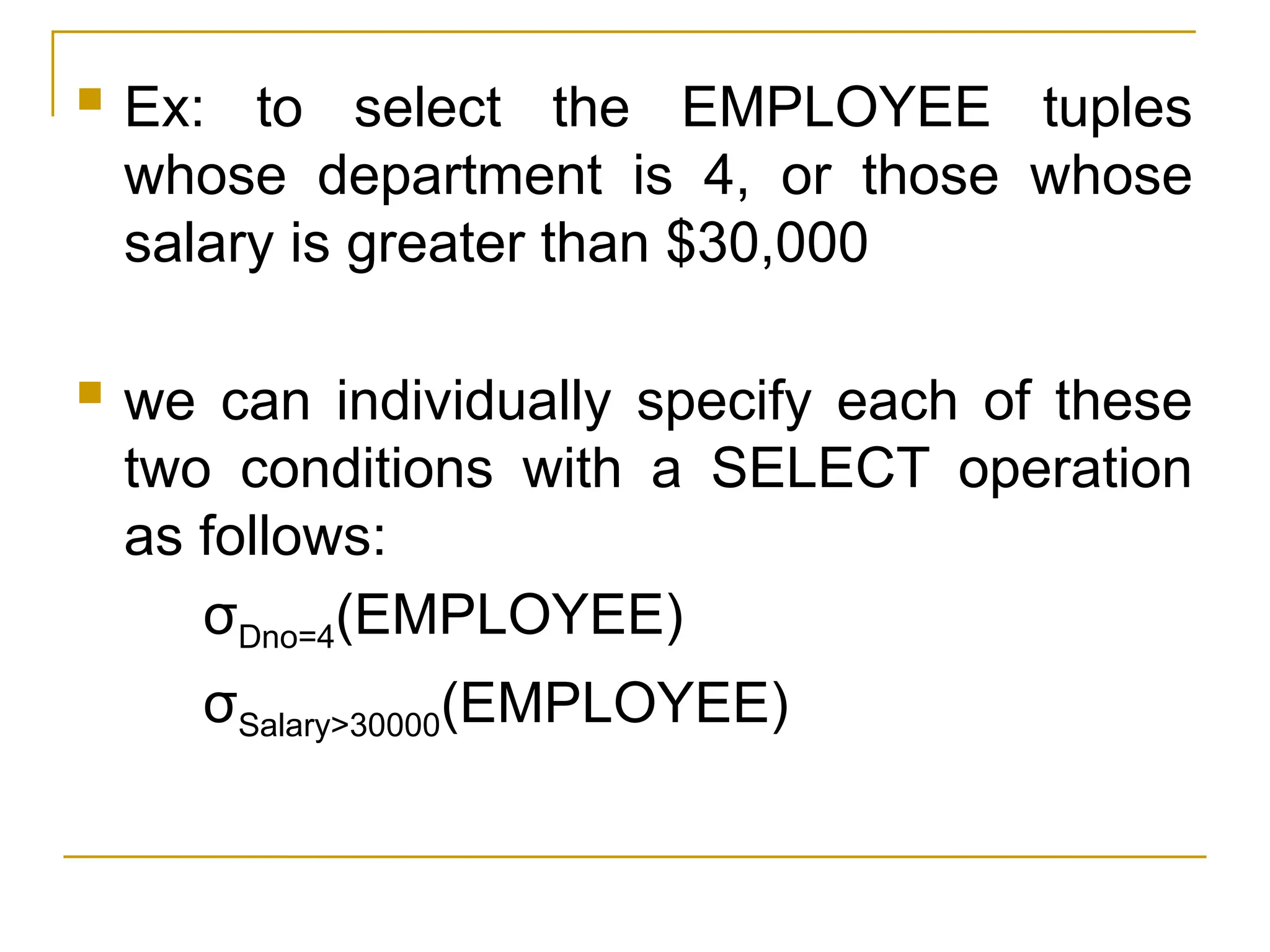
67.  Ex: to select the EMPLOYEE tuples
whose department is 4, or those whose
salary is greater than $30,000
 we can individually specify each of these
two conditions with a SELECT operation
as follows:
σDno=4(EMPLOYEE)
σSalary>30000(EMPLOYEE)

68.  Ex: to select the tuples for all employees who either
work in department 4 and make over $25,000 per
year, or work in department 5 and make over
$30,000
σ (Dno=4 AND Salary>25000) OR (Dno=5 AND Salary>30000) (EMPLOYEE)

69.  The SELECT operator is unary; that is, it is
applied to a single relation.
 The selection operation is applied to each tuple
individually; hence, selection conditions cannot
involve more than one tuple.
 The number of tuples in the resulting relation is
always less than or equal to the number of
tuples in R.
 The fraction of tuples selected by a selection
condition is referred to as the selectivity of the
condition.

70.  Notice that the SELECT operation is commutative; that
is,
σ <cond1> (σ <cond2> (R)) = σ <cond2> (σ <cond1> (R))
 Hence, a sequence of SELECTs can be applied in any
order.
 In addition, we can always combine a cascade (or
sequence) of SELECT operations into a single SELECT
operation with a conjunctive (AND) condition; that is,
 σ<cond1>(σ<cond2>(...(σ<condn>(R)) ...)) = σ<cond1>
AND<cond2> AND...AND <condn>(R

71.  In SQL, the SELECT condition is typically
specified in the WHERE clause of a query.
 For example, the following operation:
σDno=4 AND Salary>25000 (EMPLOYEE)
 SQL query:
SELECT *
FROM EMPLOYEE
WHERE Dno=4 AND Salary>25000;

72. The PROJECT Operation
 The SELECT operation chooses some of the
rows from the table while discarding other rows.
 The PROJECT operation, on the other hand,
selects certain columns from the table and
discards the other columns.
 If we are interested in only certain attributes of a
relation, we use the PROJECT operation to
project the relation over these attributes only.
 Therefore, the result of the PROJECT operation
can be visualized as a vertical partition of the
relation into two relations

73.  The general form of the PROJECT operation is
π <attribute list> (R)
where π (pi) is the symbol used to represent the
PROJECT operation,
<attribute list> is the desired sublist of attributes
from the attributes of relation R.
 The result of the PROJECT operation has only
the attributes specified in <attribute list> in the
same order as they appear in the list. Hence, its
degree is equal to the number of attributes in
<attribute list>.

74.  Ex: To list each employee’s first and last name
and salary,
π Lname, Fname, Salary (EMPLOYEE)

75.  If the attribute list includes only non key
attributes of R, duplicate tuples are likely to
occur.
 The PROJECT operation removes any
duplicate tuples, so the result of the
PROJECT operation is a set of distinct
tuples, and hence a valid relation.
 This is known as duplicate elimination.
 Ex:
π Sex, Salary (EMPLOYEE)

76.  In SQL, the PROJECT attribute list is specified
in the SELECT clause of a query.
 Ex: π job, Salary (EMPLOYEE)
 SQL query:
SELECT DISTINCT Job, Salary
FROM EMPLOYEE
 Notice that if we remove the keyword DISTINCT
from this SQL query, then duplicates will not be
eliminated.

77. Sequences of Operations and the RENAME
Operation
 In general, for most queries, we need to apply
several relational algebra operations one after
the other.
 Either we can write the operations as a single
relational algebra expression by nesting the
operations, or we can apply one operation at a
time and create intermediate result relations.
 In the latter case, we must give names to the
relations that hold the intermediate results.

78.  Ex: Retrieve the first name, last name, and
salary of all employees who work in department
number 5.
π Fname, Lname, Salary (σ Dno=5 (EMPLOYEE))
- Known as In-line expression

79.  Alternatively, we can explicitly show the
sequence of operations, giving a name to
each intermediate relation, as follows:
DEP5_EMPS ← σ Dno=5 (EMPLOYEE)
RESULT ← πFname, Lname, Salary (DEP5_EMPS)
 It is sometimes simpler to break down a complex
sequence of operations by specifying
intermediate result relations than to write a
single relational algebra expression.
 We can also use this technique to rename the
attributes in the intermediate and result relations

80.  To rename the attributes in a relation, we list the
new attribute names in parentheses.
Ex: TEMP ← σ Dno=5 (EMPLOYEE)
R(First_name, Last_name, Salary) ← π Fname, Lname, Salary
(TEMP)

81.  If no renaming is applied, the names of the
attributes in the resulting relation of a SELECT
operation are the same as those in the original
relation and in the same order.
 For a PROJECT operation with no renaming, the
resulting relation has the same attribute names
as those in the projection list and in the same
order in which they appear in the list.
 A formal RENAME operation—which can
rename either the relation name or the attribute
names, or both—as a unary operator.

82.  The general RENAME operation when applied to
a relation R of degree n is denoted by any of the
following three forms:
ρS (B1, B2, ..., Bn) (R) - renames both the relation and its attributes
ρS(R) – renames the relation only
ρ( B1, B2, ..., Bn) (R) - renames the attributes only
 where the symbol ρ (rho) is used to denote the
RENAME operator, S is the new relation name,
and B1, B2, ..., Bn are the new attribute names.
 If the attributes of R are (A1, A2, ..., An) in that
order, then each Ai is renamed as Bi.

83.  Renaming in SQL is accomplished by aliasing
using AS
 Ex:
SELECT E.Fname AS First_name, E.Lname AS
Last_name, E.Salary AS Salary
FROM EMPLOYEE AS E
WHERE E.Dno=5,

84. Relational Algebra Operations from Set Theory
- The UNION, INTERSECTION, and MINUS
Operations
 Ex: Retrieve the Social Security numbers of all
employees who either work in department 5 or
directly supervise an employee who works in
department 5
 Using UNION operation; As a single relational
algebra expression
Result ← π Ssn (σ Dno=5 (EMPLOYEE) ) ∪
π Super_ssn (σ Dno=5 (EMPLOYEE)

85.  DEP5_EMPS ← σ Dno=5 (EMPLOYEE)
 RESULT1 ← π Ssn (DEP5_EMPS)
 RESULT2 (Ssn) ← π Super_ssn (DEP5_EMPS)
 RESULT ← RESULT1 RESULT2
∪
 The relation RESULT1 has the Ssn of all employees who
work in department 5,
 RESULT2 has the Ssn of all employees who directly
supervise an employee who works in department 5.
 The UNION operation produces the tuples that are in
either RESULT1 or RESULT2 or both

86.  Set theoretic operations are used to merge the
elements of two sets in various ways:
UNION,
INTERSECTION, and
SET DIFFERENCE (also called MINUS or EXCEPT)
 These are binary operations; that is, each is applied
to two sets (of tuples).
 When these operations are adapted to relational
databases, the two relations on which any of these
three operations are applied must have the same
type of tuples; this condition has been called union
compatibility or type compatibility.

87.  Two relations R(A1, A2, ..., An) and S(B1, B2, ...,
Bn) are said to be union compatible (or type
compatible) if they have the same degree n and
if dom(Ai) = dom(Bi) for 1 ≤ i ≤ n.
 This means that the two relations have the same
number of attributes and each corresponding
pair of attributes has the same domain.

88.  We can define the three operations UNION,
INTERSECTION, and SET DIFFERENCE on two
union-compatible relations R and S as follows:
 UNION: The result of this operation, denoted by
R ∪ S, is a relation that includes all tuples that are
either in R or in S or in both R and S. Duplicate
tuples are eliminated.
 INTERSECTION: The result of this operation,
denoted by R ∩ S, is a relation that includes all
tuples that are in both R and S.
 SET DIFFERENCE (or MINUS): The result of this
operation, denoted by R – S, is a relation that
includes all tuples that are in R but not in S.

89.  STUDENT INSTRUCTOR
∪
- The names of all students and
Instructors.
- The duplicate tuples appear
only once in the result

90.  (c) STUDENT ∩ INSTRUCTOR
Includes only those who are both
students and instructors.
 Notice that both UNION and INTERSECTION are
commutative operations; that is,
R ∪ S = S ∪ R and R ∩ S = S ∩ R
 Both UNION and INTERSECTION can be treated as
n-ary operations applicable to any number of relations
because both are also associative operations; that is,
R (
∪ S ∪ T) = (R ∪ S) ∪ T and (R ∩ S ) ∩ T = R ∩ (S ∩ T )

91.  (d) STUDENT − INSTRUCTOR
- The names of students who
are not instructors
 (e) INSTRUCTOR − STUDENT
- The names of instructors who
are not students
 The MINUS operation is not commutative; that
is, in general,
R − S ≠ S − R

92. Union Operation – Example
 Relations r, s:
 r  s:
A B



1
2
1
A B


2
3
r
s
A B




1
2
1
3

93. Set-Intersection Operation – Example
 Relation r, s:
 r  s
A B



1
2
1
A B


2
3
r s
A B
 2

94. Set Difference Operation – Example
 Relations r, s:
 r – s:
A B



1
2
1
A B


2
3
r
s
A B


1
1

95. The CARTESIAN PRODUCT (CROSS PRODUCT)
Operation
 CARTESIAN PRODUCT operation—also known as
CROSS PRODUCT or CROSS JOIN—which is denoted
by X.
 This is also a binary set operation, but the relations on
which it is applied do not have to be union compatible.
 In its binary form, this set operation produces a new
element by combining every member (tuple) from one
relation (set) with every member (tuple) from the other
relation (set).
 In general, the result of R(A1, A2, ..., An) × S(B1, B2, ...,
Bm) is a relation Q with degree n + m attributes Q(A1,
A2, ..., An, B1, B2, ..., Bm), in that order.

96. Cartesian-Product Operation – Example
 Relations r, s:
 r x s:
A B


1
2
A B








1
1
1
1
2
2
2
2
C D








10
10
20
10
10
10
20
10
E
a
a
b
b
a
a
b
b
C D




10
10
20
10
E
a
a
b
b
r
s

97. Composition of Operations
 Can build expressions using multiple
operations
 Example: A=C(r x s)
 r x s
 A=C(r x s)
1
1
1
1
2
2
2
2








A B C D E








10
10
20
10
10
10
20
10
a
a
b
b
a
a
b
b
A B C D E



1
2
2



10
10
20
a
a
b

98.  Ex: To retrieve a list of names of each female employee’s
dependents.
FEMALE_EMPS ← σ Sex=‘F’ (EMPLOYEE)
EMPNAMES ← π Fname, Lname, Ssn (FEMALE_EMPS)
EMP_DEPENDENTS ← EMPNAMES × DEPENDENT
ACTUAL_DEPENDENTS ← σ Ssn=Essn (EMP_DEPENDENTS)
RESULT ← π Fname, Lname, Dependent_name
(ACTUAL_DEPENDENTS)

101. • The CARTESIAN PRODUCT creates tuples with the
combined attributes of two relations.
• We can SELECT related tuples only from the two
relations by specifying an appropriate selection condition
after the Cartesian product.
• In SQL, CARTESIAN PRODUCT can be realized by using
the CROSS JOIN option in joined tables. Alternatively, if
there are two tables in the WHERE clause and there is no
corresponding join condition in the query, the result will
also be the CARTESIAN PRODUCT of the two tables

102. Binary Relational Operations: JOIN and DIVISION
The JOIN Operation
 The JOIN operation, denoted by , is used to
combine related tuples from two relations into
single “longer” tuples.
 This operation is very important for any
relational database with more than a single
relation because it allows us to process
relationships among relations.

103. Ex: To get the manager’s name
DEPT_MGR ← DEPARTMENT Mgr_ssn=Ssn EMPLOYEE
RESULT ← π Dname, Lname, Fname (DEPT_MGR)

104. Ex:
EMP_DEPENDENTS ← EMPNAMES × DEPENDENT
ACTUAL_DEPENDENTS ← σ Ssn=Essn (EMP_DEPENDENTS)
 These two operations can be replaced with a single JOIN
operation as follows:
ACTUAL_DEPENDENTS ← EMPNAMES Ssn=Essn DEPENDENT
 The general form of a JOIN operation on two relations R(A1,
A2, ..., An) and S(B1, B2, ..., Bm) is
R <join condition> S

105. Variations of JOIN: The EQUIJOIN
and NATURAL JOIN
EQUIJOIN
 A JOIN, where the comparison operator = is
used, is called an EQUI Join.
 Ex: ACTUAL_DEPENDENTS ← σ Ssn=Essn (EMP_DEPENDENTS)
 In the result of an EQUIJOIN we always have
one or more pairs of attributes that have
identical values in every tuple

106. Ex: ACTUAL_DEPENDENTS ← σ Ssn=Essn (EMP_DEPENDENTS)

107. NATURAL JOIN
 Denoted by *
 NATURAL JOIN requires that the two join
attributes (or each pair of join attributes) have
the same name in both relations.
 If this is not the case, a renaming operation is
applied first.

108. PROJ_DEPT ← PROJECT * ρ (Dname, Dnum, Mgr_ssn, Mgr_start_date) (DEPARTMENT)
The same query can be done in two steps by creating an intermediate table
DEPT as follows:
DEPT ← ρ (Dname, Dnum, Mgr_ssn, Mgr_start_date) (DEPARTMENT)
PROJ_DEPT ← PROJECT * DEPT

109.  The attribute Dnum is called the join attribute
for the NATURAL JOIN operation, because it is
the only attribute with the same name in both
relations.

110.  If the attributes on which the natural join is
specified already have the same names in
both relations, renaming is unnecessary.
Ex:
DEPT_LOCS ← DEPARTMENT * DEPT_LOCATIONS

111.  A more general, but nonstandard definition
for NATURAL JOIN is
Q ← R *(<list1>),(<list2>)S
 In this case, <list1> specifies a list of i
attributes from R, and <list2> specifies a list
of i attributes from S.
 The lists are used to form equality
comparison conditions between pairs of
corresponding attributes, and the conditions
are then ANDed together

112.  Note: If no combination of tuples satisfies the
join condition, the result of a JOIN is an
empty relation with zero tuples.
 A single JOIN operation is used to combine
data from two relations so that related
information can be presented in a single
table.
 These operations are also known as inner
joins, to distinguish them from a different join
variation called outer joins.

113.  For a NATURAL JOIN operation R * S, only tuples
from R that have matching tuples in S—and vice
versa—appear in the result.
 Hence, tuples without a matching (or related) tuple
are eliminated from the JOIN result.
 Tuples with NULL values in the join attributes are also
eliminated.
 This type of join, where tuples with no match are
eliminated, is known as an inner join.
 In SQL, JOIN can be realized in several different
ways. The first method is to specify the <join
conditions> in the WHERE clause, along with any
other selection conditions.

114. Consider the below schema:
• lives(pname, street, city)
• works(pname, cname, salary)
• located-in(cname, city)
• manages(pname, mname)
Where, pname is a person-name, cname is
company-name, and mname is manager-name.
Write the query in relational algebra for the
following:
1) List the name of the people who work for the
company ‘CISCO’

115. 2) Find the name of persons working at ‘IBM’ who
earn more than Rs. 50,000.
3) Find the name and city of all persons who work
for ‘IBM’ and earn more than 50,000.
4) Find names of all persons who live in the same
city as the company they work for.
5) Find names of all persons who do not work for
‘IBM’.

116. Natural Join Operation – Example
 Relations r, s:
A B





1
2
4
1
2
C D





a
a
b
a
b
B
1
3
1
2
3
D
a
a
a
b
b
E





r
A B





1
1
1
1
2
C D





a
a
a
a
b
E





s
 r s

117. The DIVISION Operation
 The DIVISION operation, denoted by ÷
 In general, the DIVISION operation is applied to two
relations R(Z) ÷ S(X), where the attributes of R are a
subset of the attributes of S; that is, X ⊆ Z
 Let Y be the set of attributes of R that are not
attributes of S; that is, Y = Z – X (and hence Z = X ∪
Y).

118.  Note that in the formulation of the DIVISION
operation, the tuples in the denominator relation
S restrict the numerator relation R by selecting
those tuples in the result that match all values
present in the denominator.
 Most RDBMS implementations with SQL as the
primary query language do not directly implement
division.

119.  The DIVISION operation can be expressed
as a sequence of π, ×, and – operations as
follows:
 T1 ← πY (R)
 T2 ← π Y ((S × T1) – R)
 T ← T1 – T2
 Where Y = Z – X

120. T  R  S

121. Division Operator (÷): Division operator A÷B can
be applied if and only if:
 Attributes of B is proper subset of Attributes of A.
 The relation returned by division operator will
have attributes = (All attributes of A – All
Attributes of B)
 The relation returned by division operator will
return those tuples from relation A which are
associated to every B’s tuple.

122.  Ex: Retrieve the names of employees who work on all
the projects that ‘John Smith’ works on.
 Using the DIVISION operation:
First, retrieve the list of project numbers that ‘John
Smith’ works on in the intermediate relation
SMITH_PNOS:
SMITH ← σ Fname=‘John’ AND Lname=‘Smith’ (EMPLOYEE)
SMITH_PNOS ← π Pno (WORKS_ON Essn=Ssn SMITH)

123.  SSN_PNOS ← π Essn, Pno (WORKS_ON)
 SSNS(Ssn) ← SSN_PNOS ÷ SMITH_PNOS
 RESULT ← π Fname, Lname (SSNS * EMPLOYEE)

124. Division Operation – Example
 Relations r, s:
 r  s: A
B


1
2
A B











1
2
3
1
1
1
3
4
6
1
2
r
s

125. Another Division Example
A B








a
a
a
a
a
a
a
a
C D








a
a
b
a
b
a
b
b
E
1
1
1
1
3
1
1
1
 Relations r, s:
 r  s:
D
a
b
E
1
1
A B


a
a
C


r
s

126. Ex: Find students who enrolled all
courses.
 E (Sid,Cid) / C(Cid) = S1
Sid Cid
S1 C1
S2 C1
S1 C2
S3 C2
Cid
C1
C2
Enrolled (E) Course (C )

127.  R1   Cid (Course)
 R2   Sid (Enrolled)
 R3  R1 X R2
 R4  R3 – Enrolled
 R5   Sid (R4)
 R6   Sid (Enrolled) – R5

129. Banking Example
branch (branch_name, branch_city, assets)
customer (customer_name, customer_street,
customer_city)
account (account_number, branch_name, balance)
loan (loan_number, branch_name, amount)
depositor (customer_name, account_number)
borrower (customer_name, loan_number)

130. Example Queries
 Find all loans of over $1200
 Find the loan number for each loan of an amount greater than
$1200
amount > 1200 (loan)
loan_number (amount > 1200 (loan))
 Find the names of all customers who have a loan, an account, or both,
from the bank
customer_name (borrower)  customer_name (depositor)

131. Example Queries
 Find the names of all customers who have a
loan at the Perryridge branch.
 Find the names of all customers who have a loan at the
Perryridge branch but do not have an account at any branch of
the bank.
customer_name (branch_name = “Perryridge”
(borrower.loan_number = loan.loan_number(borrower x loan))) –
customer_name(depositor)
customer_name (branch_name=“Perryridge”
(borrower.loan_number = loan.loan_number(borrower x loan)))

132. Example Queries
 Find the names of all customers who have a
loan at the Perryridge branch.
 Query 2
customer_name(loan.loan_number = borrower.loan_number (
(branch_name = “Perryridge” (loan)) x borrower))
 Query 1
customer_name (branch_name = “Perryridge” (
borrower.loan_number = loan.loan_number (borrower x loan)))

133. Examples of Queries in Relational Algebra
 Query 1. Retrieve the name and address of all employees
who work for the ‘Research’ department.
RESEARCH_DEPT ← σ Dname=‘Research (DEPARTMENT)
RESEARCH_EMPS ← (RESEARCH_DEPT Dnumber=Dno
EMPLOYEE)
RESULT ← π Fname, Lname, Address (RESEARCH_EMPS)
 As a single in-line expression, this query becomes:
π Fname, Lname, Address (σ Dname=‘Research’ (DEPARTMENT Dnumber=Dno
(EMPLOYEE))

134.  Query 2. For every project located in ‘Stafford’, list the
project number, the controlling department number, and
the department manager’s last name, address, and birth
date.
STAFFORD_PROJS ← σ Plocation=‘Stafford’ (PROJECT)
CONTR_DEPTS ← (STAFFORD_PROJS Dnum=Dnumber
DEPARTMENT)
PROJ_DEPT_MGRS ← (CONTR_DEPTS Mgr_ssn=Ssn
EMPLOYEE)
RESULT ← π Pnumber, Dnum, Lname, Address, Bdate
(PROJ_DEPT_MGRS)