Data mining via Linear Modeling

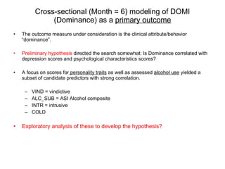
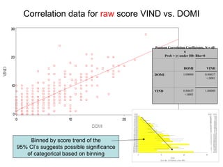
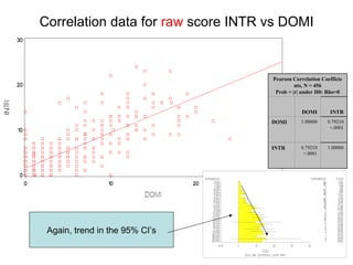
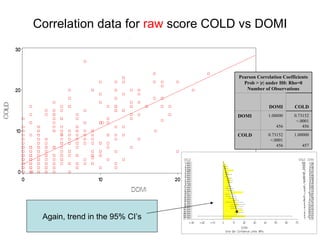
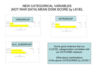
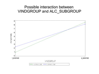
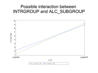
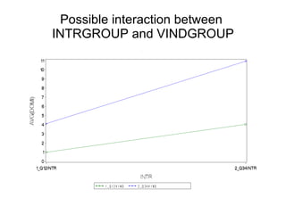
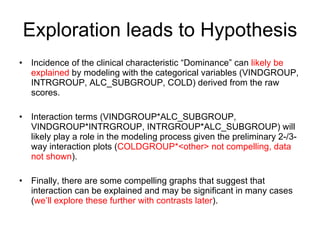
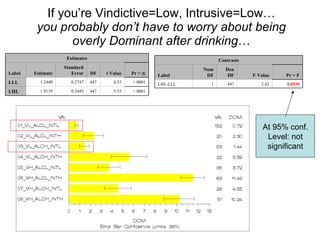
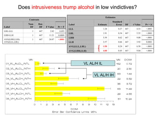
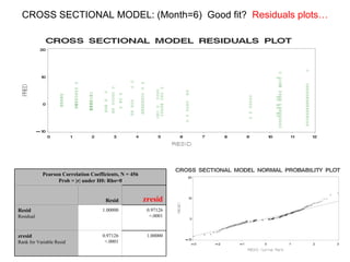
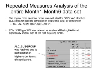
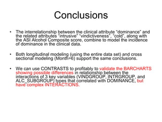
1. Factors associated with the clinical characteristic “Dominance” published in “Psychosocial Treatments for Cocaine Dependence” [Arch Gen Psychiatry 56: June 1999] Tim Hare STA531 Fall 2009

3. Correlation data for raw score VIND vs. DOMI Binned by score trend of the 95% CI’s suggests possible significance of categorical based on binning 1.00000 0.80637 <.0001 VIND 0.80637 <.0001 1.00000 DOMI VIND DOMI Pearson Correlation Coefficients, N = 456 Prob > |r| under H0: Rho=0

4. Correlation data for raw score INTR vs DOMI Again, trend in the 95% CI’s 1.00000 0.79210 <.0001 INTR 0.79210 <.0001 1.00000 DOMI INTR DOMI Pearson Correlation Coefficients, N = 456 Prob > |r| under H0: Rho=0

5. Correlation data for raw score COLD vs DOMI Again, trend in the 95% CI’s 1.00000 457 0.73152 <.0001 456 COLD 0.73152 <.0001 456 1.00000 456 DOMI COLD DOMI Pearson Correlation Coefficients Prob > |r| under H0: Rho=0 Number of Observations

7. OUTCOME MEASURE = DOMI Raw score NORMAL PROBABILITY PLOT 1.00000 0.94328 <.0001 zdomi Rank for Variable DOMI 0.94328 <.0001 1.00000 DOMI zdomi DOMI Pearson Correlation Coefficients, N = 456 Prob > |r| under H0: Rho=0

8. Potential 2-way & 3-way CROSS FACTOR GROUP VIEWS VINDGROUP-INTRGROUP VINDGROUP-ALC_SUBGROUP VINDGROUP-ALC_SUBGROUP-INTRGROUP 1) Evidence for non-homogeneous variance. 2) As well, groups are unbalanced (dissimilar counts)  USE PROC MIXED

10. NEW CATEGORICAL VARIABLES (NOT RAW DATA) MEAN DOMI SCORE by LEVEL ALC_SUBGROUP INTRGROUP VINDGROUP Some good evidence that our 2-LEVEL categorization correlates with our OUTCOME measure. What about combinations of the above CATEGORIES by LEVEL?

11. 2-way- & 3-way CROSS FACTOR GROUPS MEAN DOMI SCORES (VIND*INTR) (VIND*ALC_SUB) VIND*ALC_SUB*INTR Good story to explore… What about “interaction”???

12. Possible interaction between VINDGROUP and ALC_SUBGROUP

13. Possible interaction between INTRGROUP and ALC_SUBGROUP

14. Possible interaction between INTRGROUP and VINDGROUP

15. Graphical analysis to examine potential 3-WAY interaction VINDGROUP*INTRGROUP*ALC_SUBGROUP( LOW/HIGH ) ALC_SUBGROUP = LOW ALC_SUBGROUP = HIGH

16. PREVIEW for longitudinal modeling: Correlation noted in CROSS SECTIONAL (Month=6) data seems to persist across time … Therefore suspect “repeated measures” (longitudinal modeling) may model well from the same variables

18. Cross sectional (Month=6) modeling results confirm our suspicions PROC MIXED ( α =0.05) 2X/3X 0.0044 5.50 447 2 VINDGROUP*ALC_SUBGROUP*INTRGROUP 0.0027 9.11 447 1 VINDGROUP*ALC_SUBGROUP <.0001 33.72 447 1 VINDGROUP*INTRGROUP <.0001 163.16 447 1 INTRGROUP 0.0136 6.13 447 1 ALC_SUBGROUP <.0001 136.66 447 1 VINDGROUP 0.0002 13.79 447 1 COLDGROUP Pr > F F Value Den DF Num DF Effect Type 3 Tests of Fixed Effects

20. If you’re Vindictive=Low, Intrusive=Low… you probably don’t have to worry about being overly Dominant after drinking … At 95% conf. Level: not significant <.0001 5.55 447 0.3445 1.9119 LHL <.0001 4.53 447 0.2747 1.2440 LLL Pr > |t| t Value DF Standard Error Estimate Label Estimates 0.0938 2.82 447 1 LHL-LLL Pr > F F Value Den DF Num DF Label Contrasts

21. Does intrusiveness trump alcohol in low vindictives? VL AL/H IL VL AL/H IH <.0001 9.04 447 0.45 4.08 AVG(LHH,LLH) <.0001 6.58 447 0.24 1.58 AVG(LLL,LHL) 0.0001 3.92 447 0.66 2.57 LLH <.0001 9.00 447 0.62 5.59 LHH <.0001 5.55 447 0.34 1.91 LHL <.0001 4.53 447 0.27 1.24 LLL Pr > |t| t Value DF Standard Error Estimate Label Estimates <.0001 24.87 447 1 AVG(LHH,LLH)-AVG(LLL,LHL) 0.0009 11.21 447 1 LHH-LLH 0.093 2.82 447 1 LHL-LLL Pr > F F Value Den DF Num DF Label Contrasts

22. CROSS SECTIONAL MODEL: (Month=6) Good fit? Residuals plots… 1.00000 0.97126 <.0001 zresid Rank for Variable Resid 0.97126 <.0001 1.00000 Resid Residual zresid Resid Pearson Correlation Coefficients, N = 456 Prob > |r| under H0: Rho=0

24. LONGITUDINAL MODEL: Good fit? Residuals plots… 1.00000 0.95069 <.0001 zresid Rank for Variable Resid 0.95069 <.0001 1.00000 Resid Residual zresid Resid Pearson Correlation Coefficients, N = 456 Prob > |r| under H0: Rho=0

26. What about our cross sectional contrast of alcohol being trumped by intrusiveness in low vindictives? Does it still hold in the longitudinal analysis? Still significant At 95% CI <.0001 8.44 102 0.4247 3.5832 AVG(LHH,LLH) <.0001 6.74 102 0.2790 1.8806 AVG(LLL,LHL) <.0001 5.34 102 0.5583 2.9805 LLH <.0001 7.36 102 0.5689 4.1859 LHH <.0001 6.04 102 0.3452 2.0854 LHL <.0001 5.59 102 0.2996 1.6757 LLL Pr > |t| t Value DF Standard Error Estimate Label Estimates 0.0002 15.41 102 1 AVG(LHH,LLH)-AVG(LLL,LHL) 0.1069 2.65 102 1 LHH-LLH 0.2124 1.57 102 1 LHL-LLL Pr > F F Value Den DF Num DF Label Contrasts

28. Q&A