Data Analysis And Statistical Inference
Introduction:
The research question is as follows:
Did the sex of an individual affect the highest degree obtained by an individual in the year 2000?
I’m trying to find a relationship between these two variables, whether they are dependent on each other using
data anlysis and statistical inference tools.
This relationship is important to others as well as it gives us an idea about the attitude and behaviour of the
society pertaining to the highest degree obtained by an individual sex in the population. In other words, did
the sex of a person affect the highest degree achieved by that person in the year 2000?
Data:
I’m analyzing the GSS dataset for this research.
General Social Survey monitored the American societal change and it’s complexity from the year 1972 to
2012. GSS questions cover a diverse range of issues including national spending priorities, sex, degree, crime
and punishment, race relations, quality of life etc.
The cases in this survey include randomly surveyed people from America from the year 1972 to 2012 of which
I’m anlyzing the cases in the year 2000.
The variables I’m using are sex and degree.They are both categorical variables. Sex contains 2 levels and
degree contains 5 levels.
This is an observational study. This is a survey conducted by GSS and since we are not assigning any
conditions to any control, we can conclude that it is an observational study.
The population of interest includes people surveyed in the year 2000. Since this is a random survey, we can
generalize to the population but we must take into account the bias of people surveyed.The survey may not
truly reflect the opinion of the general population.
This data show a co-relation between two variables. Co-relation does not imply causation. We can imply
causation using an experimental study.
Exploratory data analysis:
Since my research question deals with the year 2000, I subset all the cases belonging to the year 2000 into a
new data frame:
newdata <- gss[gss$year==2000,]
And I’m only using the sex and degree variable, therfore I eliminate all the other columns using subset
function:
newdata <- newdata[,c(“sex”,“degree”)]
The first 10 rows of the newdata is displayed below:
## sex degree
## 38117 Male Bachelor
## 38118 Female High School
## 38119 Female High School
1
## 38120 Female High School
## 38121 Female Junior College
## 38122 Female High School
## 38123 Male High School
## 38124 Female Junior College
## 38125 Male Graduate
## 38126 Male Bachelor
I load the mass package to accomodate all rows and then use the table function to calculate the number of
males and females in each level of degree achieved:
tbl = table(newdatasex, newdatadegree)
##
## Lt High School High School Junior College Bachelor Graduate
## Male 186 624 85 191 127
## Female 233 877 121 244 91
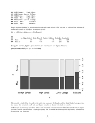
Using plot function, I plot a graph between the variables sex and degree obtained.
plot(x=newdatadegree, y = newdatasex)
x
y
Lt High School High School Junior College Graduate
MaleFemale
0.00.20.40.60.81.0
The result is a stacked bar plot, where the white bar represents the females and the dark/shaded bar represents
the males. Sex variable is on Y axis and degree variable on X axis with their own levels.
As I analyse my summary and visual data, I note that there are more number of females in each level of degree
obtained bar the graduate level.This maybe purely due to chance or there maybe a dependency relationship
between the two variables.
2
Inference:
We are trying to find a relationship between two categorical variables.
So the null hypothesis H0: Whether the sex variable is independent of the degree variable and the differences
in values is merely due to chance.
And the alternate hypothesis HA: The sex and degree variables are dependent on each other and it involves
something more than a chance.
The conditions for a Chi squared Test requires the samples to be independent observations and each case
contributes to only one cell in the table. The second condition is that each particular scenario has 5 expected
cases.
We can use only the Chi-squared Test of Independence since both the variables are categorical and the degree
variable contains 5 levels. No other test can solve for 5 levels other than Chi.
I use the in built Chi-squared function to perform the test:
chisq.test(tbl)
##
## Pearson's Chi-squared test
##
## data: tbl
## X-squared = 22.128, df = 4, p-value = 0.000189
The test returns X-squared value=22,128, df=4, p-value=0.000189.
We use a significance level of 0.05 which is a standard. The p-value we obtained is 0.000189 which is way
below 0.05.
Therefore we reject the null hypothesis which states that the two variables are independent of each other.
The data provides convincing evidence for the alternate hypothesis.
Conclusion:
I set off on this research to apply my knowledge about data analysis which I’ve learnt over the past many
weeks. I researched for a possible relationship between two variables (sex,degree), whether they affect each
other or not. I used the functions learnt to visualize and summarize data, apllied the null and alternate
hypothesis concept and performed a Chi-squared test to determine the relationship.
Initially I assumed the two variables would be independent, but the tests performed showed that the two
variables (sex,degree) were indeed dependent on each other. The statistical tests proved my assumption
wrong and in the process I learnt a great deal about analyzing data.
We can include this reseach for a large period of time, say like 15 years. Analyze the data to see whether the
differnces change when considering a very large sample.
References:
Link to GSS dataset: http://www.icpsr.umich.edu/icpsrweb/ICPSR/studies/34802/version/1
3
Appendix:
## sex degree
## 38117 Male Bachelor
## 38118 Female High School
## 38119 Female High School
## 38120 Female High School
## 38121 Female Junior College
## 38122 Female High School
## 38123 Male High School
## 38124 Female Junior College
## 38125 Male Graduate
## 38126 Male Bachelor
Author
My name is Shreyas G S. I am passionate about the potential of Data Analysis and Machine Learning. My
career goal is to be a Data Scientist.
4

Data Analysis and Statistical inference

  • 1.
    Data Analysis AndStatistical Inference Introduction: The research question is as follows: Did the sex of an individual affect the highest degree obtained by an individual in the year 2000? I’m trying to find a relationship between these two variables, whether they are dependent on each other using data anlysis and statistical inference tools. This relationship is important to others as well as it gives us an idea about the attitude and behaviour of the society pertaining to the highest degree obtained by an individual sex in the population. In other words, did the sex of a person affect the highest degree achieved by that person in the year 2000? Data: I’m analyzing the GSS dataset for this research. General Social Survey monitored the American societal change and it’s complexity from the year 1972 to 2012. GSS questions cover a diverse range of issues including national spending priorities, sex, degree, crime and punishment, race relations, quality of life etc. The cases in this survey include randomly surveyed people from America from the year 1972 to 2012 of which I’m anlyzing the cases in the year 2000. The variables I’m using are sex and degree.They are both categorical variables. Sex contains 2 levels and degree contains 5 levels. This is an observational study. This is a survey conducted by GSS and since we are not assigning any conditions to any control, we can conclude that it is an observational study. The population of interest includes people surveyed in the year 2000. Since this is a random survey, we can generalize to the population but we must take into account the bias of people surveyed.The survey may not truly reflect the opinion of the general population. This data show a co-relation between two variables. Co-relation does not imply causation. We can imply causation using an experimental study. Exploratory data analysis: Since my research question deals with the year 2000, I subset all the cases belonging to the year 2000 into a new data frame: newdata <- gss[gss$year==2000,] And I’m only using the sex and degree variable, therfore I eliminate all the other columns using subset function: newdata <- newdata[,c(“sex”,“degree”)] The first 10 rows of the newdata is displayed below: ## sex degree ## 38117 Male Bachelor ## 38118 Female High School ## 38119 Female High School 1
  • 2.
    ## 38120 FemaleHigh School ## 38121 Female Junior College ## 38122 Female High School ## 38123 Male High School ## 38124 Female Junior College ## 38125 Male Graduate ## 38126 Male Bachelor I load the mass package to accomodate all rows and then use the table function to calculate the number of males and females in each level of degree achieved: tbl = table(newdatasex, newdatadegree) ## ## Lt High School High School Junior College Bachelor Graduate ## Male 186 624 85 191 127 ## Female 233 877 121 244 91 Using plot function, I plot a graph between the variables sex and degree obtained. plot(x=newdatadegree, y = newdatasex) x y Lt High School High School Junior College Graduate MaleFemale 0.00.20.40.60.81.0 The result is a stacked bar plot, where the white bar represents the females and the dark/shaded bar represents the males. Sex variable is on Y axis and degree variable on X axis with their own levels. As I analyse my summary and visual data, I note that there are more number of females in each level of degree obtained bar the graduate level.This maybe purely due to chance or there maybe a dependency relationship between the two variables. 2
  • 3.
    Inference: We are tryingto find a relationship between two categorical variables. So the null hypothesis H0: Whether the sex variable is independent of the degree variable and the differences in values is merely due to chance. And the alternate hypothesis HA: The sex and degree variables are dependent on each other and it involves something more than a chance. The conditions for a Chi squared Test requires the samples to be independent observations and each case contributes to only one cell in the table. The second condition is that each particular scenario has 5 expected cases. We can use only the Chi-squared Test of Independence since both the variables are categorical and the degree variable contains 5 levels. No other test can solve for 5 levels other than Chi. I use the in built Chi-squared function to perform the test: chisq.test(tbl) ## ## Pearson's Chi-squared test ## ## data: tbl ## X-squared = 22.128, df = 4, p-value = 0.000189 The test returns X-squared value=22,128, df=4, p-value=0.000189. We use a significance level of 0.05 which is a standard. The p-value we obtained is 0.000189 which is way below 0.05. Therefore we reject the null hypothesis which states that the two variables are independent of each other. The data provides convincing evidence for the alternate hypothesis. Conclusion: I set off on this research to apply my knowledge about data analysis which I’ve learnt over the past many weeks. I researched for a possible relationship between two variables (sex,degree), whether they affect each other or not. I used the functions learnt to visualize and summarize data, apllied the null and alternate hypothesis concept and performed a Chi-squared test to determine the relationship. Initially I assumed the two variables would be independent, but the tests performed showed that the two variables (sex,degree) were indeed dependent on each other. The statistical tests proved my assumption wrong and in the process I learnt a great deal about analyzing data. We can include this reseach for a large period of time, say like 15 years. Analyze the data to see whether the differnces change when considering a very large sample. References: Link to GSS dataset: http://www.icpsr.umich.edu/icpsrweb/ICPSR/studies/34802/version/1 3
  • 4.
    Appendix: ## sex degree ##38117 Male Bachelor ## 38118 Female High School ## 38119 Female High School ## 38120 Female High School ## 38121 Female Junior College ## 38122 Female High School ## 38123 Male High School ## 38124 Female Junior College ## 38125 Male Graduate ## 38126 Male Bachelor Author My name is Shreyas G S. I am passionate about the potential of Data Analysis and Machine Learning. My career goal is to be a Data Scientist. 4