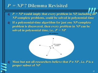
1
Lower Bounds
Lower bound: an estimate on a minimum amount of work
needed to solve a given problem
Examples:
 number of comparisons needed to find the largest element
in a set of n numbers
 number of comparisons needed to sort an array of size n
 number of comparisons necessary for searching in a sorted
array
 number of multiplications needed to multiply two n-by-n
matrices
2
Lower Bounds (cont.)
 Lower bound can be
• an exact count
• an efficiency class ()
 Tight lower bound: there exists an algorithm with the same
efficiency as the lower bound
Problem Lower bound Tightness
sorting (nlog n) yes
searching in a sorted array (log n) yes
element uniqueness (nlog n) yes
n-digit integer multiplication (n) unknown
multiplication of n-by-n matrices (n2) unknown
3
Methods for Establishing Lower Bounds
 trivial lower bounds
 information-theoretic arguments (decision trees)
 adversary arguments
 problem reduction
4
Trivial Lower Bounds
Trivial lower bounds: based on counting the number of items
that must be processed in input and generated as output
Examples
 finding max element
 polynomial evaluation
 sorting
 element uniqueness
 Hamiltonian circuit existence
Conclusions
 may and may not be useful
 be careful in deciding how many elements must be processed
5
Decision Trees
Decision tree — a convenient model of algorithms involving
comparisons in which:
 internal nodes represent comparisons
 leaves represent outcomes
Decision tree for 3-element insertion sort
a < b
b < c a < c
yes
yes no
no
yes
no
a < c b < c
a < b < c
c < a < b
b < a < c
b < c < a
no yes
abc
abc bac
bca
acb
yes
a < c < b c < b < a
no
6
Decision Trees and Sorting Algorithms
 Any comparison-based sorting algorithm can be represented
by a decision tree
 Number of leaves (outcomes)  n!
 Height of binary tree with n! leaves  log2n!
 Minimum number of comparisons in the worst case  log2n!
for any comparison-based sorting algorithm
 log2n!  n log2n
 This lower bound is tight (mergesort)
7
Adversary Arguments
Adversary argument: a method of proving a lower bound by
playing role of adversary that makes algorithm work the hardest
by adjusting input
Example 1: “Guessing” a number between 1 and n with yes/no
questions
Adversary: Puts the number in a larger of the two subsets
generated by last question
Example 2: Merging two sorted lists of size n
a1 < a2 < … < an and b1 < b2 < … < bn
Adversary: ai < bj iff i < j
Output b1 < a1 < b2 < a2 < … < bn < an requires 2n-1 comparisons
of adjacent elements
8
Lower Bounds by Problem Reduction
Idea: If problem P is at least as hard as problem Q, then a lower
bound for Q is also a lower bound for P.
Hence, find problem Q with a known lower bound that can
be reduced to problem P in question.
Example: P is finding MST for n points in Cartesian plane
Q is element uniqueness problem (known to be in (nlogn))
9
Classifying Problem Complexity
Is the problem tractable, i.e., is there a polynomial-time (O(p(n))
algorithm that solves it?
Possible answers:
 yes (give examples)
 no
• because it’s been proved that no algorithm exists at all
(e.g., Turing’s halting problem)
• because it’s been be proved that any algorithm takes
exponential time
 unknown
10
Problem Types: Optimization and Decision
 Optimization problem: find a solution that maximizes or
minimizes some objective function
 Decision problem: answer yes/no to a question
Many problems have decision and optimization versions.
E.g.: traveling salesman problem
 optimization: find Hamiltonian cycle of minimum length
 decision: find Hamiltonian cycle of length  m
Decision problems are more convenient for formal investigation
of their complexity.
11
Class P
P: the class of decision problems that are solvable in O(p(n))
time, where p(n) is a polynomial of problem’s input size n
Examples:
 searching
 element uniqueness
 graph connectivity
 graph acyclicity
 primality testing (finally proved in 2002)
12
Class NP
NP (nondeterministic polynomial): class of decision problems
whose proposed solutions can be verified in polynomial time
= solvable by a nondeterministic polynomial algorithm
A nondeterministic polynomial algorithm is an abstract two-stage
procedure that:
 generates a random string purported to solve the problem
 checks whether this solution is correct in polynomial time
By definition, it solves the problem if it’s capable of generating
and verifying a solution on one of its tries
Why this definition?
 led to development of the rich theory called “computational
complexity”
13
Example: CNF satisfiability
Problem: Is a boolean expression in its conjunctive normal
form (CNF) satisfiable, i.e., are there values of its
variables that makes it true?
This problem is in NP. Nondeterministic algorithm:
 Guess truth assignment
 Substitute the values into the CNF formula to see if it
evaluates to true
Example: (A | ¬B | ¬C) & (A | B) & (¬B | ¬D | E) & (¬D | ¬E)
Truth assignments:
A B C D E
0 0 0 0 0
. . .
1 1 1 1 1
Checking phase: O(n)
14
What problems are in NP?
 Hamiltonian circuit existence
 Partition problem: Is it possible to partition a set of n
integers into two disjoint subsets with the same sum?
 Decision versions of TSP, knapsack problem, graph
coloring, and many other combinatorial optimization
problems. (Few exceptions include: MST, shortest paths)
 All the problems in P can also be solved in this manner (no
guessing is necessary), so we have:
P  NP
 Big question: P = NP ?
15
NP-Complete Problems
A decision problem D is NP-complete if it’s as hard as any
problem in NP, i.e.,
 D is in NP
 every problem in NP is polynomial-time reducible to D
Cook’s theorem (1971): CNF-sat is NP-complete
NP-complete
problem
NP problems
16
NP-Complete Problems (cont.)
Other NP-complete problems obtained through polynomial-
time reductions from a known NP-complete problem
Examples: TSP, knapsack, partition, graph-coloring and
hundreds of other problems of combinatorial nature
know n
NP-complete
problem
NP problems
candidate
for NP -
completeness
17
P = NP ? Dilemma Revisited
 P = NP would imply that every problem in NP, including all
NP-complete problems, could be solved in polynomial time
 If a polynomial-time algorithm for just one NP-complete
problem is discovered, then every problem in NP can be
solved in polynomial time, i.e., P = NP
 Most but not all researchers believe that P  NP , i.e. P is a
proper subset of NP
NP-complete
problem
NP problems

Confidence interval two tail tests-lower bounds upperbounds

  • 1.
    1 Lower Bounds Lower bound:an estimate on a minimum amount of work needed to solve a given problem Examples:  number of comparisons needed to find the largest element in a set of n numbers  number of comparisons needed to sort an array of size n  number of comparisons necessary for searching in a sorted array  number of multiplications needed to multiply two n-by-n matrices
  • 2.
    2 Lower Bounds (cont.) Lower bound can be • an exact count • an efficiency class ()  Tight lower bound: there exists an algorithm with the same efficiency as the lower bound Problem Lower bound Tightness sorting (nlog n) yes searching in a sorted array (log n) yes element uniqueness (nlog n) yes n-digit integer multiplication (n) unknown multiplication of n-by-n matrices (n2) unknown
  • 3.
    3 Methods for EstablishingLower Bounds  trivial lower bounds  information-theoretic arguments (decision trees)  adversary arguments  problem reduction
  • 4.
    4 Trivial Lower Bounds Triviallower bounds: based on counting the number of items that must be processed in input and generated as output Examples  finding max element  polynomial evaluation  sorting  element uniqueness  Hamiltonian circuit existence Conclusions  may and may not be useful  be careful in deciding how many elements must be processed
  • 5.
    5 Decision Trees Decision tree— a convenient model of algorithms involving comparisons in which:  internal nodes represent comparisons  leaves represent outcomes Decision tree for 3-element insertion sort a < b b < c a < c yes yes no no yes no a < c b < c a < b < c c < a < b b < a < c b < c < a no yes abc abc bac bca acb yes a < c < b c < b < a no
  • 6.
    6 Decision Trees andSorting Algorithms  Any comparison-based sorting algorithm can be represented by a decision tree  Number of leaves (outcomes)  n!  Height of binary tree with n! leaves  log2n!  Minimum number of comparisons in the worst case  log2n! for any comparison-based sorting algorithm  log2n!  n log2n  This lower bound is tight (mergesort)
  • 7.
    7 Adversary Arguments Adversary argument:a method of proving a lower bound by playing role of adversary that makes algorithm work the hardest by adjusting input Example 1: “Guessing” a number between 1 and n with yes/no questions Adversary: Puts the number in a larger of the two subsets generated by last question Example 2: Merging two sorted lists of size n a1 < a2 < … < an and b1 < b2 < … < bn Adversary: ai < bj iff i < j Output b1 < a1 < b2 < a2 < … < bn < an requires 2n-1 comparisons of adjacent elements
  • 8.
    8 Lower Bounds byProblem Reduction Idea: If problem P is at least as hard as problem Q, then a lower bound for Q is also a lower bound for P. Hence, find problem Q with a known lower bound that can be reduced to problem P in question. Example: P is finding MST for n points in Cartesian plane Q is element uniqueness problem (known to be in (nlogn))
  • 9.
    9 Classifying Problem Complexity Isthe problem tractable, i.e., is there a polynomial-time (O(p(n)) algorithm that solves it? Possible answers:  yes (give examples)  no • because it’s been proved that no algorithm exists at all (e.g., Turing’s halting problem) • because it’s been be proved that any algorithm takes exponential time  unknown
  • 10.
    10 Problem Types: Optimizationand Decision  Optimization problem: find a solution that maximizes or minimizes some objective function  Decision problem: answer yes/no to a question Many problems have decision and optimization versions. E.g.: traveling salesman problem  optimization: find Hamiltonian cycle of minimum length  decision: find Hamiltonian cycle of length  m Decision problems are more convenient for formal investigation of their complexity.
  • 11.
    11 Class P P: theclass of decision problems that are solvable in O(p(n)) time, where p(n) is a polynomial of problem’s input size n Examples:  searching  element uniqueness  graph connectivity  graph acyclicity  primality testing (finally proved in 2002)
  • 12.
    12 Class NP NP (nondeterministicpolynomial): class of decision problems whose proposed solutions can be verified in polynomial time = solvable by a nondeterministic polynomial algorithm A nondeterministic polynomial algorithm is an abstract two-stage procedure that:  generates a random string purported to solve the problem  checks whether this solution is correct in polynomial time By definition, it solves the problem if it’s capable of generating and verifying a solution on one of its tries Why this definition?  led to development of the rich theory called “computational complexity”
  • 13.
    13 Example: CNF satisfiability Problem:Is a boolean expression in its conjunctive normal form (CNF) satisfiable, i.e., are there values of its variables that makes it true? This problem is in NP. Nondeterministic algorithm:  Guess truth assignment  Substitute the values into the CNF formula to see if it evaluates to true Example: (A | ¬B | ¬C) & (A | B) & (¬B | ¬D | E) & (¬D | ¬E) Truth assignments: A B C D E 0 0 0 0 0 . . . 1 1 1 1 1 Checking phase: O(n)
  • 14.
    14 What problems arein NP?  Hamiltonian circuit existence  Partition problem: Is it possible to partition a set of n integers into two disjoint subsets with the same sum?  Decision versions of TSP, knapsack problem, graph coloring, and many other combinatorial optimization problems. (Few exceptions include: MST, shortest paths)  All the problems in P can also be solved in this manner (no guessing is necessary), so we have: P  NP  Big question: P = NP ?
  • 15.
    15 NP-Complete Problems A decisionproblem D is NP-complete if it’s as hard as any problem in NP, i.e.,  D is in NP  every problem in NP is polynomial-time reducible to D Cook’s theorem (1971): CNF-sat is NP-complete NP-complete problem NP problems
  • 16.
    16 NP-Complete Problems (cont.) OtherNP-complete problems obtained through polynomial- time reductions from a known NP-complete problem Examples: TSP, knapsack, partition, graph-coloring and hundreds of other problems of combinatorial nature know n NP-complete problem NP problems candidate for NP - completeness
  • 17.
    17 P = NP? Dilemma Revisited  P = NP would imply that every problem in NP, including all NP-complete problems, could be solved in polynomial time  If a polynomial-time algorithm for just one NP-complete problem is discovered, then every problem in NP can be solved in polynomial time, i.e., P = NP  Most but not all researchers believe that P  NP , i.e. P is a proper subset of NP NP-complete problem NP problems