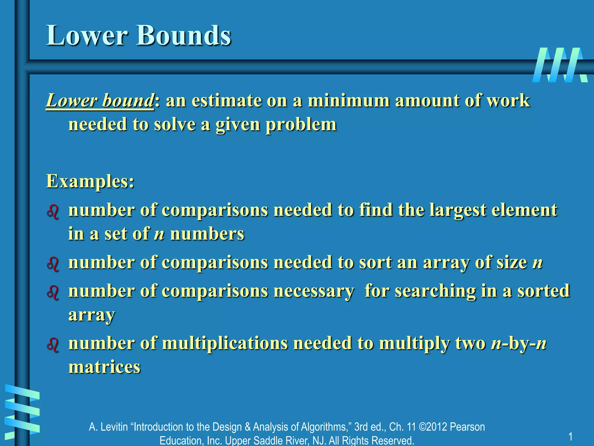
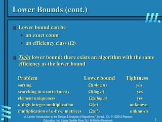
The document discusses lower bounds for algorithms. It defines lower bounds as estimates of the minimum amount of work needed to solve a problem. It then provides examples of problems and their known lower bounds, such as sorting requiring Ω(nlogn) comparisons. The document outlines several methods for establishing lower bounds, including trivial counting arguments, decision trees, adversary arguments, and reducing other problems. It focuses on using reductions to show that one problem is at least as hard as another known hard problem to prove a new lower bound. The summary concludes by briefly introducing the concept of NP-complete problems.

1. A. Levitin “Introduction to the Design & Analysis of Algorithms,” 3rd ed., Ch. 11 ©2012 Pearson
Education, Inc. Upper Saddle River, NJ. All Rights Reserved. 1
Lower Bounds
Lower bound: an estimate on a minimum amount of work
needed to solve a given problem
Examples:
 number of comparisons needed to find the largest element
in a set of n numbers
 number of comparisons needed to sort an array of size n
 number of comparisons necessary for searching in a sorted
array
 number of multiplications needed to multiply two n-by-n
matrices

2. A. Levitin “Introduction to the Design & Analysis of Algorithms,” 3rd ed., Ch. 11 ©2012 Pearson
Education, Inc. Upper Saddle River, NJ. All Rights Reserved. 2
Lower Bounds (cont.)
 Lower bound can be
• an exact count
• an efficiency class ()
 Tight lower bound: there exists an algorithm with the same
efficiency as the lower bound
Problem Lower bound Tightness
sorting (nlog n) yes
searching in a sorted array (log n) yes
element uniqueness (nlog n) yes
n-digit integer multiplication (n) unknown
multiplication of n-by-n matrices (n2) unknown

3. A. Levitin “Introduction to the Design & Analysis of Algorithms,” 3rd ed., Ch. 11 ©2012 Pearson
Education, Inc. Upper Saddle River, NJ. All Rights Reserved. 3
Methods for Establishing Lower Bounds
 trivial lower bounds
 information-theoretic arguments (decision trees)
 adversary arguments (SKIP)
 problem reduction

4. A. Levitin “Introduction to the Design & Analysis of Algorithms,” 3rd ed., Ch. 11 ©2012 Pearson
Education, Inc. Upper Saddle River, NJ. All Rights Reserved. 4
Trivial Lower Bounds
Trivial lower bounds: based on counting the number of items
that must be processed in input and generated as output
Examples
 finding max element
 polynomial evaluation
 sorting
 element uniqueness
 Hamiltonian circuit existence
Conclusions
 may and may not be useful
 be careful in deciding how many elements must be processed (min-max)

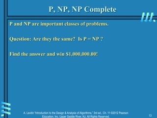
5. A. Levitin “Introduction to the Design & Analysis of Algorithms,” 3rd ed., Ch. 11 ©2012 Pearson
Education, Inc. Upper Saddle River, NJ. All Rights Reserved. 5
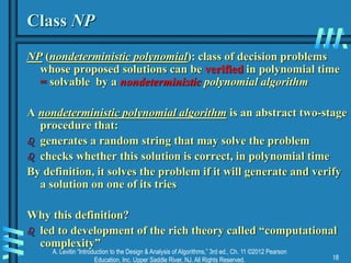
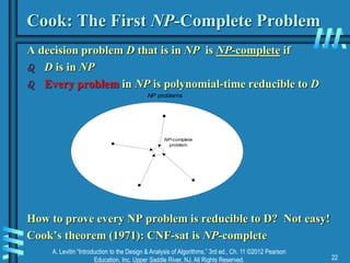
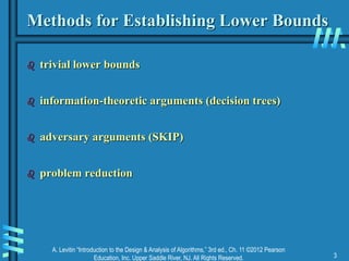
Decision Trees
Decision tree —model algorithms that use comparisons:
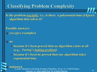
 internal nodes represent comparisons
 leaves represent outcomes
 How many orderings of 2 elements? Of 3? Of n?
 Tree for 3-element insertion sort [insert b in a, then c into ab]
a < b
b < c a < c
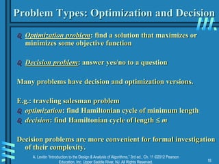
yes
yes no
no
yes
no
a < c b < c
a < b < c
c < a < b
b < a < c
b < c < a
no yes
abc
abc bac
bca
acb
yes
a < c < b c < b < a
no

6. A. Levitin “Introduction to the Design & Analysis of Algorithms,” 3rd ed., Ch. 11 ©2012 Pearson
Education, Inc. Upper Saddle River, NJ. All Rights Reserved. 6
Decision Trees and Sorting Algorithms
 Any comparison-based sorting algorithm can be represented
by a decision tree
 Number of leaves (outcomes)  n!
 Height of binary tree with n! leaves  log2n!
 Minimum number of comparisons in the worst case  log2n!
for any comparison-based sorting algorithm
 log23! = log2 6 = 3
 log2n!  n log2n, for large n
 This lower bound is tight (mergesort)

7. A. Levitin “Introduction to the Design & Analysis of Algorithms,” 3rd ed., Ch. 11 ©2012 Pearson
Education, Inc. Upper Saddle River, NJ. All Rights Reserved. 7
Adversary Arguments (SKIP)
Adversary argument: a method of proving a lower bound by
playing role of adversary that makes algorithm work the hardest
by adjusting input
Example 1: “Guessing” a number between 1 and n with yes/no
questions
Adversary: Puts the number in a larger of the two subsets
generated by last question
Example 2: Merging two sorted lists of size n
a1 < a2 < … < an and b1 < b2 < … < bn
Adversary: ai < bj iff i < j
Output b1 < a1 < b2 < a2 < … < bn < an requires 2n-1 comparisons
of adjacent elements

8. A. Levitin “Introduction to the Design & Analysis of Algorithms,” 3rd ed., Ch. 11 ©2012 Pearson
Education, Inc. Upper Saddle River, NJ. All Rights Reserved. 8
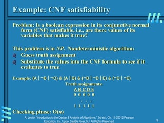
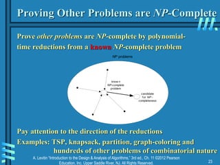
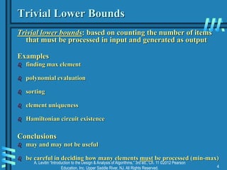
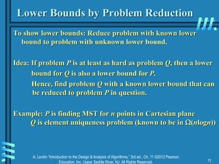
Lower Bounds by Problem Reduction
If we know a LB for alg A, can we use that knowledge to find a
LB for alg B? Remember reduction:
- Minheap reduces to maxheap
- Minimum reduces to sort
- Element uniqueness for pairs reduces to closest pair
Which would be most useful?
A [(f )] reduces to B [(? )]
B [(? )] reduces to A [(f )]
[Assume the reduction itself is fast (ie O(f)) ]

9. A. Levitin “Introduction to the Design & Analysis of Algorithms,” 3rd ed., Ch. 11 ©2012 Pearson
Education, Inc. Upper Saddle River, NJ. All Rights Reserved. 9
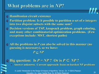
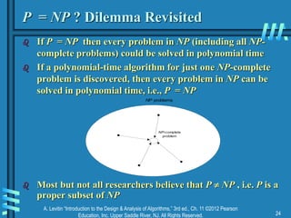
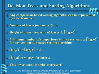
Lower Bounds by Problem Reduction
Which would be most useful?
A [(f )] reduces to B [(? )]
B [(? )] reduces to A [(f )]
Proc A [(f )] Proc B [(? )]
… …
B [(? )] A [(f )]
… …
A= [(? )] => ??? A = [(? )] => ???

10. A. Levitin “Introduction to the Design & Analysis of Algorithms,” 3rd ed., Ch. 11 ©2012 Pearson
Education, Inc. Upper Saddle River, NJ. All Rights Reserved. 10
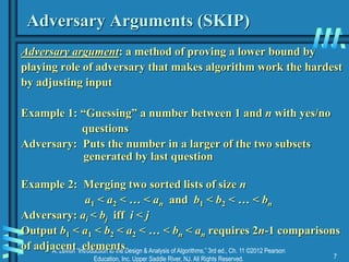
Lower Bounds by Problem Reduction
Which would be most useful?
A [(f )] reduces to B [(? )]
B [(? )] reduces to A [(f )]
Proc A [(f )] Proc B [(? )]
… …
B [(? )] A [(f )]
… …
A= [(f )] => B = [(f )] A = [(f )] => Nothing

11. A. Levitin “Introduction to the Design & Analysis of Algorithms,” 3rd ed., Ch. 11 ©2012 Pearson
Education, Inc. Upper Saddle River, NJ. All Rights Reserved. 11
Lower Bounds by Problem Reduction
To show lower bounds: Reduce problem with known lower
bound to problem with unknown lower bound.
Idea: If problem P is at least as hard as problem Q, then a lower
bound for Q is also a lower bound for P.
Hence, find problem Q with a known lower bound that can
be reduced to problem P in question.
Example: P is finding MST for n points in Cartesian plane
Q is element uniqueness problem (known to be in (nlogn))

12. A. Levitin “Introduction to the Design & Analysis of Algorithms,” 3rd ed., Ch. 11 ©2012 Pearson
Education, Inc. Upper Saddle River, NJ. All Rights Reserved. 12
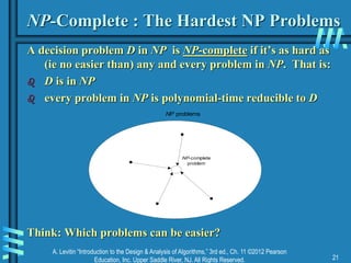
Lower Bounds by Problem Reduction
Example: P is finding MST for n points in Cartesian plane
Q is element uniqueness problem (known to be in (nlogn))
Reduce Element Uniqueness to MST:
Unique (S : IntSet = {x1, x2, …, xn}) [Known (nlogn)]
P : PairSet = {(x1, 0), (x2, 0), …, (xn, 0)}
T : Tree = MST (P)
D : Nat = min_length (edges of T)
return D = 0
Thus, MST is (nlogn)!

13. A. Levitin “Introduction to the Design & Analysis of Algorithms,” 3rd ed., Ch. 11 ©2012 Pearson
Education, Inc. Upper Saddle River, NJ. All Rights Reserved. 13
P, NP, NP Complete
P and NP are important classes of problems.
Question: Are they the same? Is P = NP ?
Find the answer and win $1,000,000.00!

14. A. Levitin “Introduction to the Design & Analysis of Algorithms,” 3rd ed., Ch. 11 ©2012 Pearson
Education, Inc. Upper Saddle River, NJ. All Rights Reserved. 14
Basic Concepts
- Classifying Problems
- Tractable and non-tractable
- Optimization and Decision Problems
- Problem Classes
- P
- NP
- NP Complete

15. A. Levitin “Introduction to the Design & Analysis of Algorithms,” 3rd ed., Ch. 11 ©2012 Pearson
Education, Inc. Upper Saddle River, NJ. All Rights Reserved. 15
Classifying Problem Complexity
Is the problem tractable, i.e., is there a polynomial-time (O(p(n))
algorithm that solves it?
Possible answers:
 yes (give examples)
 no
• because it’s been proved that no algorithm exists at all
(e.g., Turing’s halting problem)
• because it’s been be proved that any algorithm takes
exponential time
 unknown

16. A. Levitin “Introduction to the Design & Analysis of Algorithms,” 3rd ed., Ch. 11 ©2012 Pearson
Education, Inc. Upper Saddle River, NJ. All Rights Reserved. 16
Problem Types: Optimization and Decision
 Optimization problem: find a solution that maximizes or
minimizes some objective function
 Decision problem: answer yes/no to a question
Many problems have decision and optimization versions.
E.g.: traveling salesman problem
 optimization: find Hamiltonian cycle of minimum length
 decision: find Hamiltonian cycle of length  m
Decision problems are more convenient for formal investigation
of their complexity.

17. A. Levitin “Introduction to the Design & Analysis of Algorithms,” 3rd ed., Ch. 11 ©2012 Pearson
Education, Inc. Upper Saddle River, NJ. All Rights Reserved. 17
Class P
P: the class of decision problems that are solvable in O(p(n))
time, where p(n) is a polynomial of problem’s input size n
Examples:
 searching
 element uniqueness
 graph connectivity
 graph acyclicity
 primality testing (finally proved in 2002)

18. A. Levitin “Introduction to the Design & Analysis of Algorithms,” 3rd ed., Ch. 11 ©2012 Pearson
Education, Inc. Upper Saddle River, NJ. All Rights Reserved. 18
Class NP
NP (nondeterministic polynomial): class of decision problems
whose proposed solutions can be verified in polynomial time
= solvable by a nondeterministic polynomial algorithm
A nondeterministic polynomial algorithm is an abstract two-stage
procedure that:
 generates a random string that may solve the problem
 checks whether this solution is correct, in polynomial time
By definition, it solves the problem if it will generate and verify
a solution on one of its tries
Why this definition?
 led to development of the rich theory called “computational
complexity”

19. A. Levitin “Introduction to the Design & Analysis of Algorithms,” 3rd ed., Ch. 11 ©2012 Pearson
Education, Inc. Upper Saddle River, NJ. All Rights Reserved. 19
Example: CNF satisfiability
Problem: Is a boolean expression in its conjunctive normal
form (CNF) satisfiable, i.e., are there values of its
variables that makes it true?
This problem is in NP. Nondeterministic algorithm:
 Guess truth assignment
 Substitute the values into the CNF formula to see if it
evaluates to true
Example: (A | ¬B | ¬C) & (A | B) & (¬B | ¬D | E) & (¬D | ¬E)
Truth assignments:
A B C D E
0 0 0 0 0
. . .
1 1 1 1 1
Checking phase: O(n)

20. A. Levitin “Introduction to the Design & Analysis of Algorithms,” 3rd ed., Ch. 11 ©2012 Pearson
Education, Inc. Upper Saddle River, NJ. All Rights Reserved. 20
What problems are in NP?
 Hamiltonian circuit existence
 Partition problem: Is it possible to partition a set of n integers
into two disjoint subsets with the same sum?
 Decision versions of TSP, knapsack problem, graph coloring,
and many other combinatorial optimization problems. (Few
exceptions include: MST, shortest paths)
 All the problems in P can also be solved in this manner (no
guessing is necessary), so we have:
P  NP
 Big question: Is P = NP ? Or is P ⊂ NP ?
• Answer unknown. Current approach: focus on hardest NP problems

21. A. Levitin “Introduction to the Design & Analysis of Algorithms,” 3rd ed., Ch. 11 ©2012 Pearson
Education, Inc. Upper Saddle River, NJ. All Rights Reserved. 21
NP-Complete : The Hardest NP Problems
A decision problem D in NP is NP-complete if it’s as hard as
(ie no easier than) any and every problem in NP. That is:
 D is in NP
 every problem in NP is polynomial-time reducible to D
Think: Which problems can be easier?
NP-complete
problem
NP problems

22. A. Levitin “Introduction to the Design & Analysis of Algorithms,” 3rd ed., Ch. 11 ©2012 Pearson
Education, Inc. Upper Saddle River, NJ. All Rights Reserved. 22
Cook: The First NP-Complete Problem
A decision problem D that is in NP is NP-complete if
 D is in NP
 Every problem in NP is polynomial-time reducible to D
How to prove every NP problem is reducible to D? Not easy!
Cook’s theorem (1971): CNF-sat is NP-complete
NP-complete
problem
NP problems

23. A. Levitin “Introduction to the Design & Analysis of Algorithms,” 3rd ed., Ch. 11 ©2012 Pearson
Education, Inc. Upper Saddle River, NJ. All Rights Reserved. 23
Proving Other Problems are NP-Complete
Prove other problems are NP-complete by polynomial-
time reductions from a known NP-complete problem
Pay attention to the direction of the reductions
Examples: TSP, knapsack, partition, graph-coloring and
hundreds of other problems of combinatorial nature
know n
NP-complete
problem
NP problems
candidate
for NP -
completeness

24. A. Levitin “Introduction to the Design & Analysis of Algorithms,” 3rd ed., Ch. 11 ©2012 Pearson
Education, Inc. Upper Saddle River, NJ. All Rights Reserved. 24
P = NP ? Dilemma Revisited
 If P = NP then every problem in NP (including all NP-
complete problems) could be solved in polynomial time
 If a polynomial-time algorithm for just one NP-complete
problem is discovered, then every problem in NP can be
solved in polynomial time, i.e., P = NP
 Most but not all researchers believe that P  NP , i.e. P is a
proper subset of NP
NP-complete
problem
NP problems