Brain Structure
Brain Structure
Containsaround 10,000,000,000 neurons
Contains around 10,000,000,000 neurons
• Approx. the number of raindrops to fill an
Approx. the number of raindrops to fill an
olympic swimming pool
olympic swimming pool
Each of which is connected to around
Each of which is connected to around
10,000 others
10,000 others
Neurons communicate through synapses –
Neurons communicate through synapses –
effectively a configurable chemical
effectively a configurable chemical
junction between neurons
junction between neurons
3.
Neurons
Neurons
Neuron systemsfor signal processing and
memory
Connectionism was proposed based on the
research outcome in neuron science about how
the information is processed, stored and
communicated among neurons.
1. A brain is composed of trillions of cells which
interact with each other
2. A cell is composed of three parts
(a) Dendritic tree: receive signals
(b) Cell body: process signals
(c) Axon: transmit signals
Neuronal Function
Neuronal Function
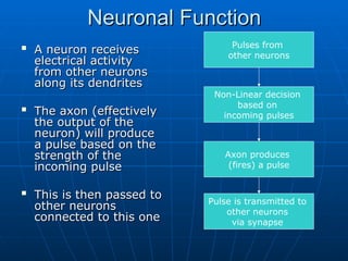
Aneuron receives
A neuron receives
electrical activity
electrical activity
from other neurons
from other neurons
along its dendrites
along its dendrites
The axon (effectively
The axon (effectively
the output of the
the output of the
neuron) will produce
neuron) will produce
a pulse based on the
a pulse based on the
strength of the
strength of the
incoming pulse
incoming pulse
This is then passed to
This is then passed to
other neurons
other neurons
connected to this one
connected to this one
Pulses from
other neurons
Non-Linear decision
based on
incoming pulses
Axon produces
(fires) a pulse
Pulse is transmitted to
other neurons
via synapse
6.
Creating Learning Machines
CreatingLearning Machines
There are a number of desirable properties we as
There are a number of desirable properties we as
humans possess
humans possess
However, clearly we have very different hardware
However, clearly we have very different hardware
to computers
to computers
Some (moderately successful) attempts have
Some (moderately successful) attempts have
been made to recreate neural architecture in
been made to recreate neural architecture in
hardware
hardware
However, the most popular method is to simulate
However, the most popular method is to simulate
neural processes on a standard computer –
neural processes on a standard computer –
neural networks
neural networks
7.
The Beginning
The Beginning
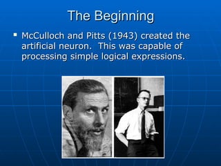
McCullochand Pitts (1943) created the
McCulloch and Pitts (1943) created the
artificial neuron. This was capable of
artificial neuron. This was capable of
processing simple logical expressions.
processing simple logical expressions.
Hebbian Learning (1949)
HebbianLearning (1949)
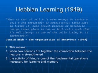
“When an axon of cell A is near enough to excite a
cell B and repeatedly or persistently takes part
in firing it, some growth process or metabolic
change takes place in one or both cells such that
A’s efficiency, as one of the cells firing B, is
increased.”1
Donald Hebb – The Organisation of Behaviour (1949)
This means:
1. when two neurons fire together the connection between the
neurons is strengthened
2. the activity of firing is one of the fundamental operations
necessary for learning and memory
10.
Rosenblatt’s Perceptron
Rosenblatt’s Perceptron
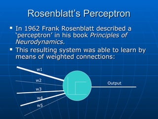
In 1962 Frank Rosenblatt described a
In 1962 Frank Rosenblatt described a
‘perceptron’ in his book
‘perceptron’ in his book Principles of
Principles of
Neurodynamics.
Neurodynamics.
This resulting system was able to learn by
This resulting system was able to learn by
means of weighted connections:
means of weighted connections:
Output
w1
w2
w3
w4
w5
11.
Problems with thePerceptron
Problems with the Perceptron
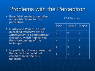
Rosenblatt made some rather
Rosenblatt made some rather
outlandish claims for the
outlandish claims for the
perceptron
perceptron
Minsky and Papert in 1969
Minsky and Papert in 1969
published
published Perceptrons: An
Perceptrons: An
Introduction to Computational
Introduction to Computational
Geometry
Geometry which highlighted
which highlighted
the shortcomings of the
the shortcomings of the
technique
technique
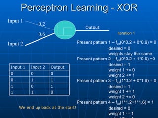
In particular, it was shown that
In particular, it was shown that
the perceptron could not
the perceptron could not
correctly solve the XOR
correctly solve the XOR
function:
function:
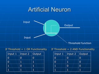
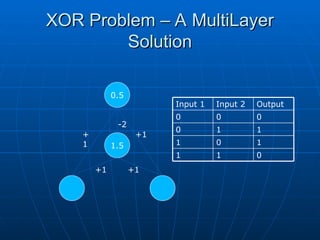
Input 1
Input 1 Input 2
Input 2 Output
Output
0
0 0
0 0
0
0
0 1
1 1
1
1
1 0
0 1
1
1
1 1
1 0
0
XOR Function
12.
Dark Ages forNeural Computing
Dark Ages for Neural Computing
Two paradigms of AI research presented
Two paradigms of AI research presented
themselves:
themselves:
• The classical symbolic method
The classical symbolic method
• The non-classical connectionist (neural)
The non-classical connectionist (neural)
method
method
Due to Minsky and Papert’s arguments,
Due to Minsky and Papert’s arguments,
hardly any research was conducted into
hardly any research was conducted into
neural computing until the 1980s….
neural computing until the 1980s….
13.
1986 - aResurgence in
1986 - a Resurgence in
Connectionism
Connectionism
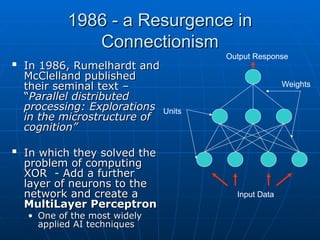
In 1986, Rumelhardt and
In 1986, Rumelhardt and
McClelland published
McClelland published
their seminal text –
their seminal text –
“
“Parallel distributed
Parallel distributed
processing: Explorations
processing: Explorations
in the microstructure of
in the microstructure of
cognition”
cognition”
In which they solved the
In which they solved the
problem of computing
problem of computing
XOR - Add a further
XOR - Add a further
layer of neurons to the
layer of neurons to the
network and create a
network and create a
MultiLayer Perceptron
MultiLayer Perceptron
• One of the most widely
One of the most widely
applied AI techniques
applied AI techniques
Units
Input Data
Output Response
Weights
14.
Applications of NeuralComputing
Applications of Neural Computing
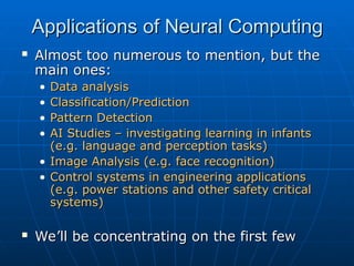
Almost too numerous to mention, but the
Almost too numerous to mention, but the
main ones:
main ones:
• Data analysis
Data analysis
• Classification/Prediction
Classification/Prediction
• Pattern Detection
Pattern Detection
• AI Studies – investigating learning in infants
AI Studies – investigating learning in infants
(e.g. language and perception tasks)
(e.g. language and perception tasks)
• Image Analysis (e.g. face recognition)
Image Analysis (e.g. face recognition)
• Control systems in engineering applications
Control systems in engineering applications
(e.g. power stations and other safety critical
(e.g. power stations and other safety critical
systems)
systems)
We’ll be concentrating on the first few
We’ll be concentrating on the first few
15.
Variations on thePerceptron
Variations on the Perceptron
Multi-Layer Perceptrons
Multi-Layer Perceptrons
Recurrent Neural Networks
Recurrent Neural Networks
Self-Organising Maps
Self-Organising Maps
Kohonen Networks
Kohonen Networks
Boltzmann Machines
Boltzmann Machines
Probabilistic Neural Networks
Probabilistic Neural Networks
Many more…
Many more…
16.
Neural Computing/Connectionism
Neural Computing/Connectionism
Summary
Summary
Computational paradigm based loosely on the
Computational paradigm based loosely on the
workings of the human brain – not exactly
workings of the human brain – not exactly
(temporal effects are ignored)
(temporal effects are ignored)
Have shown to have human-like qualities, also
Have shown to have human-like qualities, also
making similar mistakes (e.g. optical illusions)
making similar mistakes (e.g. optical illusions)
Have a significantly different method of
Have a significantly different method of
computation than traditional rule-based AI.
computation than traditional rule-based AI.
Have been successfully used in a huge number of
Have been successfully used in a huge number of
application areas
application areas
17.
Learning in NeuralNetworks
Learning in Neural Networks
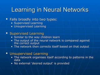
Falls broadly into two types:
Falls broadly into two types:
• Supervised Learning
Supervised Learning
• Unsupervised Learning
Unsupervised Learning
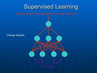
Supervised Learning
Supervised Learning
• Similar to the way children learn
Similar to the way children learn
• The output of the neural network is compared against
The output of the neural network is compared against
the correct output
the correct output
• The network then corrects itself based on that output
The network then corrects itself based on that output
Unsupervised Learning
Unsupervised Learning
• The network organises itself according to patterns in the
The network organises itself according to patterns in the
data
data
• No external 'desired output' is provided
No external 'desired output' is provided
18.
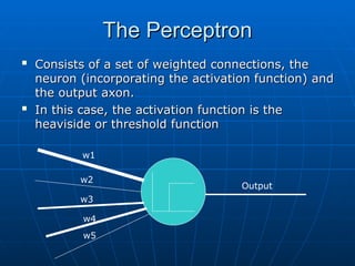
The Perceptron
The Perceptron
Consistsof a set of weighted connections, the
Consists of a set of weighted connections, the
neuron (incorporating the activation function) and
neuron (incorporating the activation function) and
the output axon.
the output axon.
In this case, the activation function is the
In this case, the activation function is the
heaviside or threshold function
heaviside or threshold function
Output
w1
w2
w3
w4
w5
19.
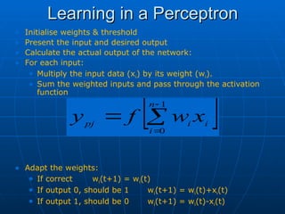
Learning in aPerceptron
Learning in a Perceptron
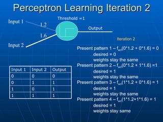
• Initialise weights & threshold
• Present the input and desired output
• Calculate the actual output of the network:
• For each input:
• Multiply the input data (xi) by its weight (wi).
• Sum the weighted inputs and pass through the activation
function
• Adapt the weights:
• If correct wi(t+1) = wi(t)
• If output 0, should be 1 wi(t+1) = wi(t)+xi(t)
• If output 1, should be 0 wi(t+1) = wi(t)-xi(t)
1
0
n
i
i
i
pj
x
w
f
y
Modified Versions ofLearning
Modified Versions of Learning
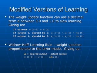
The weight update function can use a decimal
The weight update function can use a decimal
term
term η
η between 0.0 and 1.0 to slow learning.
between 0.0 and 1.0 to slow learning.
Giving us:
Giving us:
If correct
If correct w
wi
i(t+1) = w
(t+1) = wi
i(t)
(t)
If output 0, should be 1:
If output 0, should be 1: w
wi
i(t+1) = w
(t+1) = wi
i(t) +
(t) + η
ηx
xi
i(t)
(t)
If output 1, should be 0:
If output 1, should be 0: w
wi
i(t+1) = w
(t+1) = wi
i(t) -
(t) - η
ηx
xi
i(t)
(t)
Widrow-Hoff Learning Rule – weight updates
Widrow-Hoff Learning Rule – weight updates
proportionate to the error made. Giving us:
proportionate to the error made. Giving us:
Δ
Δ = desired output – actual output
= desired output – actual output
w
wi
i(t+1) = w
(t+1) = wi
i(t) +
(t) + η
ηΔ
Δx
xi
i(t)
(t)
24.
Limitations of thePerceptron
Limitations of the Perceptron
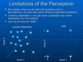
No matter what we do with the learning rule in
No matter what we do with the learning rule in
perceptrons, we can only solve linearly separable problems
perceptrons, we can only solve linearly separable problems
Linearly separable = we can draw a straight line which
Linearly separable = we can draw a straight line which
separates our two classes
separates our two classes
Can we do this for XOR?
Can we do this for XOR?
Linearly Separable
Input 1
Input
2
0 1
0
1
XOR
Input 1
Input
2
25.
MultiLayer Perceptron
MultiLayer Perceptron
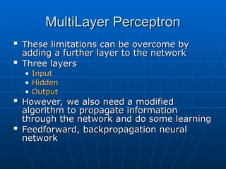
Theselimitations can be overcome by
These limitations can be overcome by
adding a further layer to the network
adding a further layer to the network
Three layers
Three layers
• Input
Input
• Hidden
Hidden
• Output
Output
However, we also need a modified
However, we also need a modified
algorithm to propagate information
algorithm to propagate information
through the network and do some learning
through the network and do some learning
Feedforward, backpropagation neural
Feedforward, backpropagation neural
network
network
26.
Activation Functions
Activation Functions
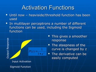
Thisgives a smoother
This gives a smoother
response
response
The steepness of the
The steepness of the
curve is changed by z
curve is changed by z
The derivative can be
The derivative can be
easily computed
easily computed
Sigmoid Function
Input Activation
Output
Response
Until now – heaviside/threshold function has been
Until now – heaviside/threshold function has been
used
used
In mutlilayer perceptrons a number of different
In mutlilayer perceptrons a number of different
functions can be used, including the Sigmoid
functions can be used, including the Sigmoid
function
function
z
e
z
P
1
1
)
(
Weights
Weights
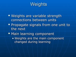
Weights are variablestrength
Weights are variable strength
connections between units
connections between units
Propagate signals from one unit to
Propagate signals from one unit to
the next
the next
Main learning component
Main learning component
• Weights are the main component
Weights are the main component
changed during learning
changed during learning
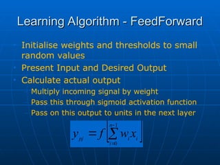
Learning Algorithm -FeedForward
Learning Algorithm - FeedForward
• Initialise weights and thresholds to small
random values
• Present Input and Desired Output
• Calculate actual output
– Multiply incoming signal by weight
– Pass this through sigmoid activation function
– Pass on this output to units in the next layer
1
0
n
i
i
i
pj
x
w
f
y
31.
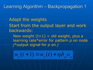
Learning Algorithm –Backpropagation 1
Learning Algorithm – Backpropagation 1
• Adapt the weights
• Start from the output layer and work
backwards:
– New weight (t+1) = old weight, plus a
learning rate*error for pattern p on node
j*output signal for p on j
pj
pj
ij
ij
o
t
w
t
w
)
(
)
1
(
32.
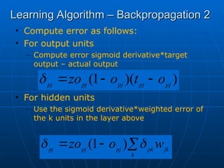
Learning Algorithm –Backpropagation 2
Learning Algorithm – Backpropagation 2
• Compute error as follows:
• For output units
– Compute error sigmoid derivative*target
output – actual output
• For hidden units
– Use the sigmoid derivative*weighted error of
the k units in the layer above
)
)(
1
( pj
pj
pj
pj
pj
o
t
o
zo
k
jk
pk
pj
pj
pj
w
o
zo
)
1
(
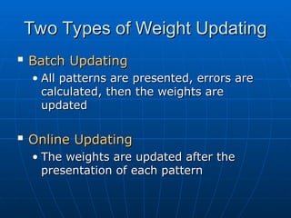
Two Types ofWeight Updating
Two Types of Weight Updating
Batch Updating
Batch Updating
• All patterns are presented, errors are
All patterns are presented, errors are
calculated, then the weights are
calculated, then the weights are
updated
updated
Online Updating
Online Updating
• The weights are updated after the
The weights are updated after the
presentation of each pattern
presentation of each pattern
Neural Network Properties
NeuralNetwork Properties
Able to relate input variables to required output
Able to relate input variables to required output
e.g.
e.g.
• Input car attributes and predict MPG
Input car attributes and predict MPG
• Predict stock market based on historical information
Predict stock market based on historical information
• Classify individuals as ‘cancerous’ and ‘non-cancerous’
Classify individuals as ‘cancerous’ and ‘non-cancerous’
based on their genes
based on their genes
• Many other control and learning tasks
Many other control and learning tasks
Is able to
Is able to generalise
generalise between samples
between samples
Shows
Shows ‘graceful degradation’
‘graceful degradation’ – removing one or
– removing one or
more units results in reduced performance, not
more units results in reduced performance, not
complete failure
complete failure


![[IJET V2I2P20] Authors: Dr. Sanjeev S Sannakki, Ms.Anjanabhargavi A Kulkarni](https://cdn.slidesharecdn.com/ss_thumbnails/ijet-v2i2p20-160609043318-thumbnail.jpg?width=640&height=640&fit=bounds)