Download to read offline


![Introduction to Algorithms & Algorithm
Analysis 11
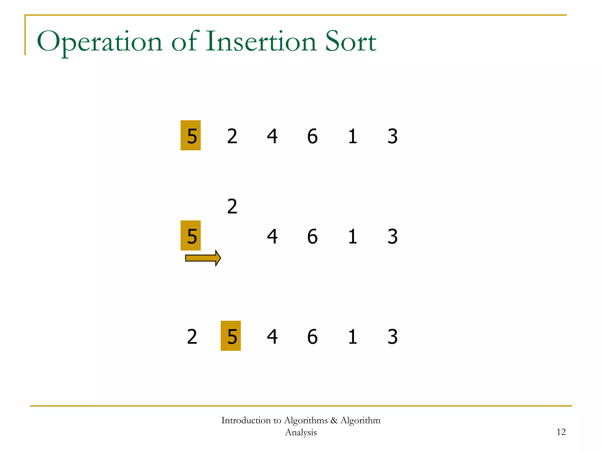
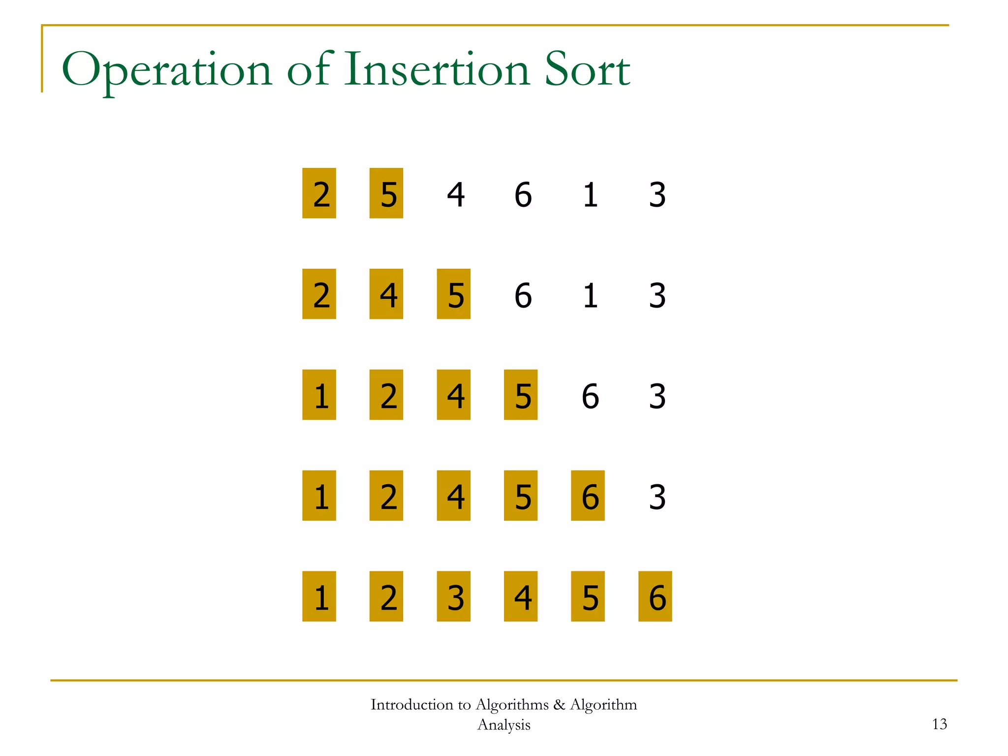
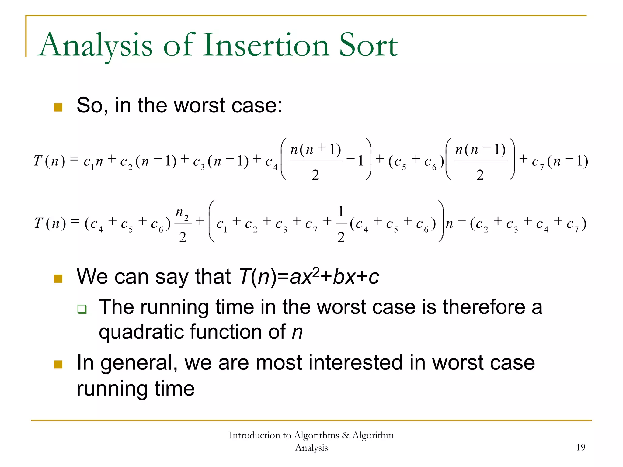
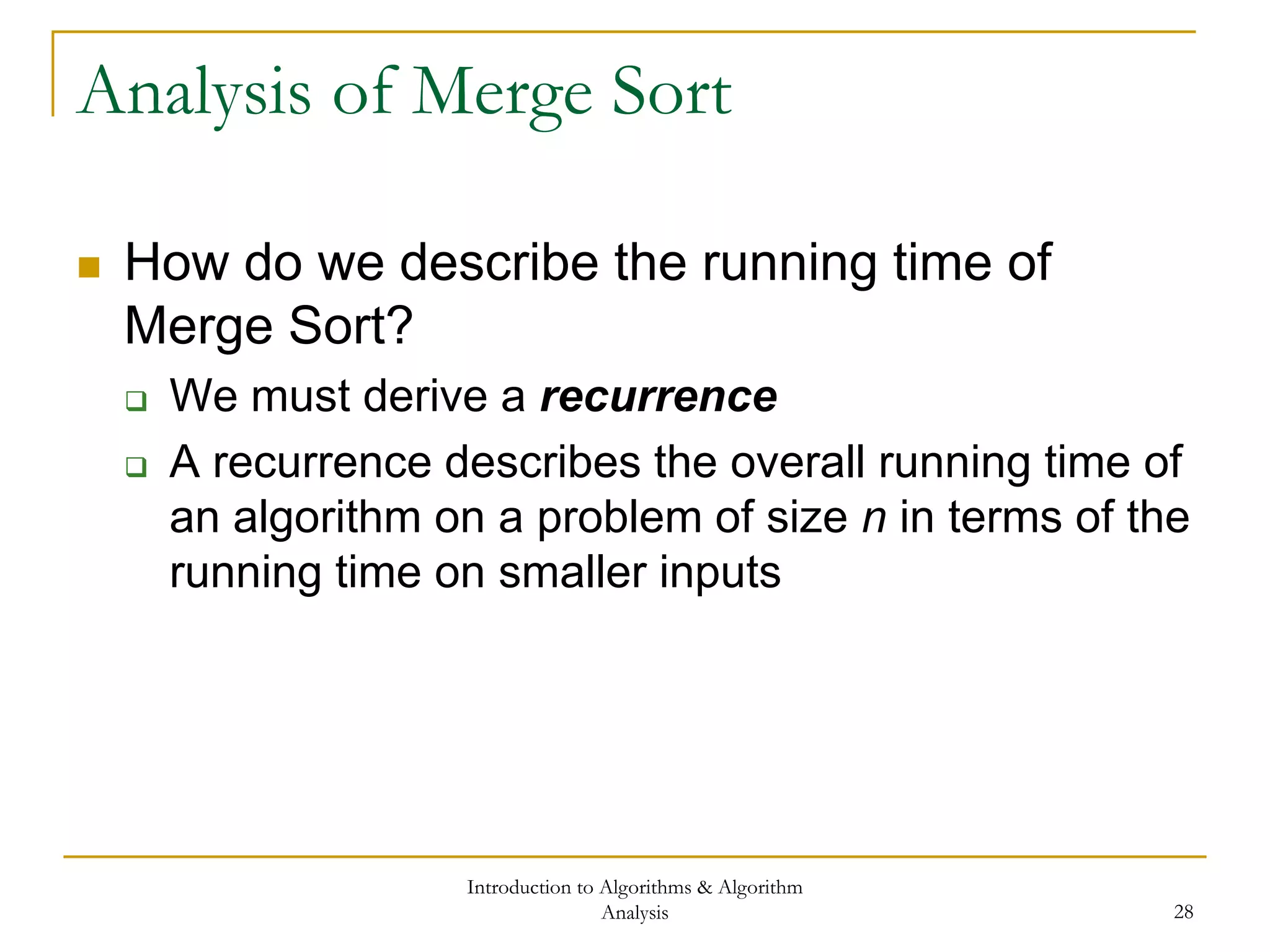
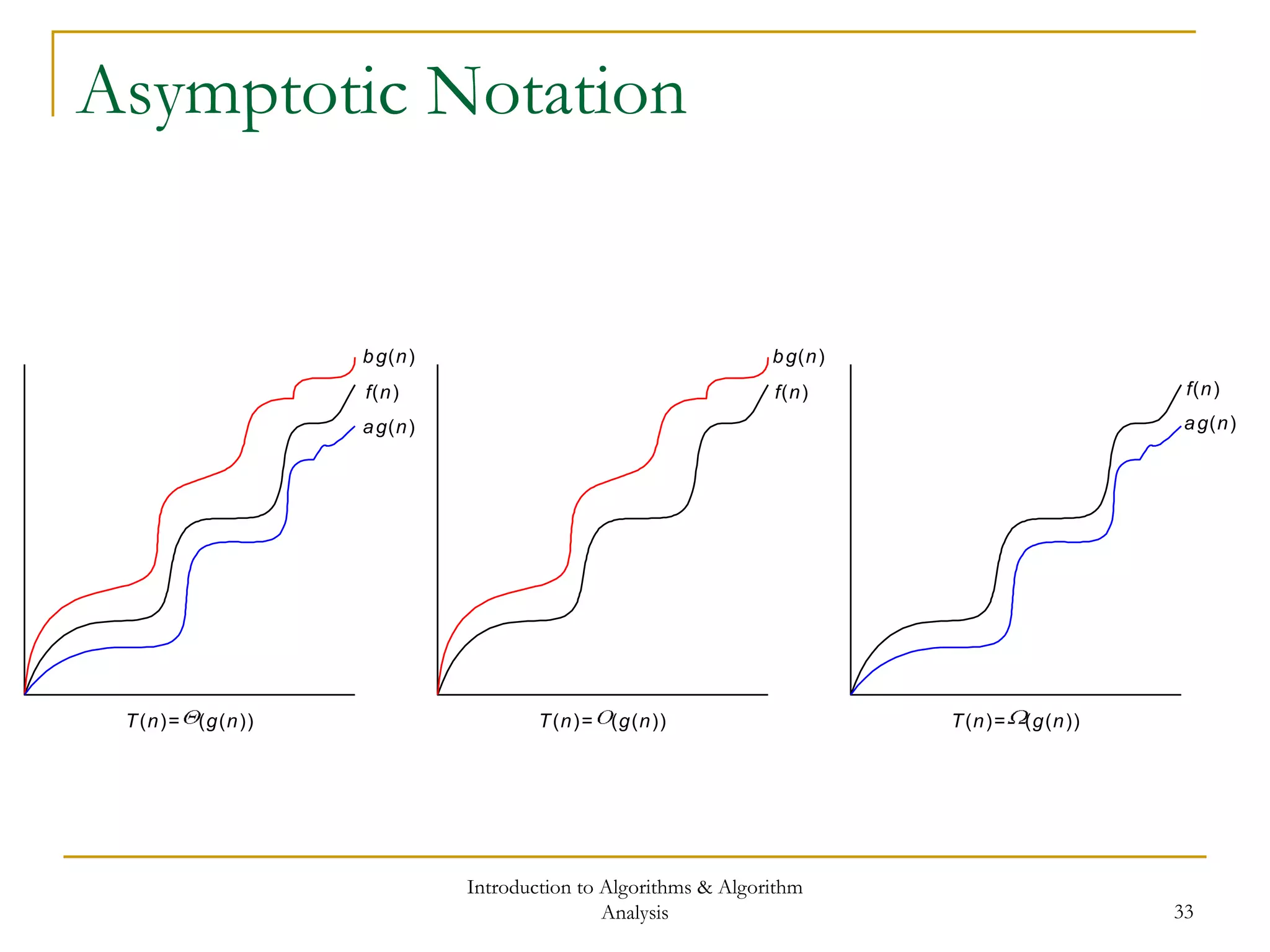
Insertion Sort: Algorithm
void InsertionSort(ArrayType A[], unsigned size)
{
for ( unsigned j = 1 ; j < size ; ++j )
{
ArrayType key = A[j];
int i = j-1;
while ( i >= 0 && A[i] > key )
{
A[i+1] = A[i];
--i;
}
A[i+1] = key;
}
}](https://image.slidesharecdn.com/cis435week01-140325170012-phpapp02/75/Cis435-week01-11-2048.jpg)
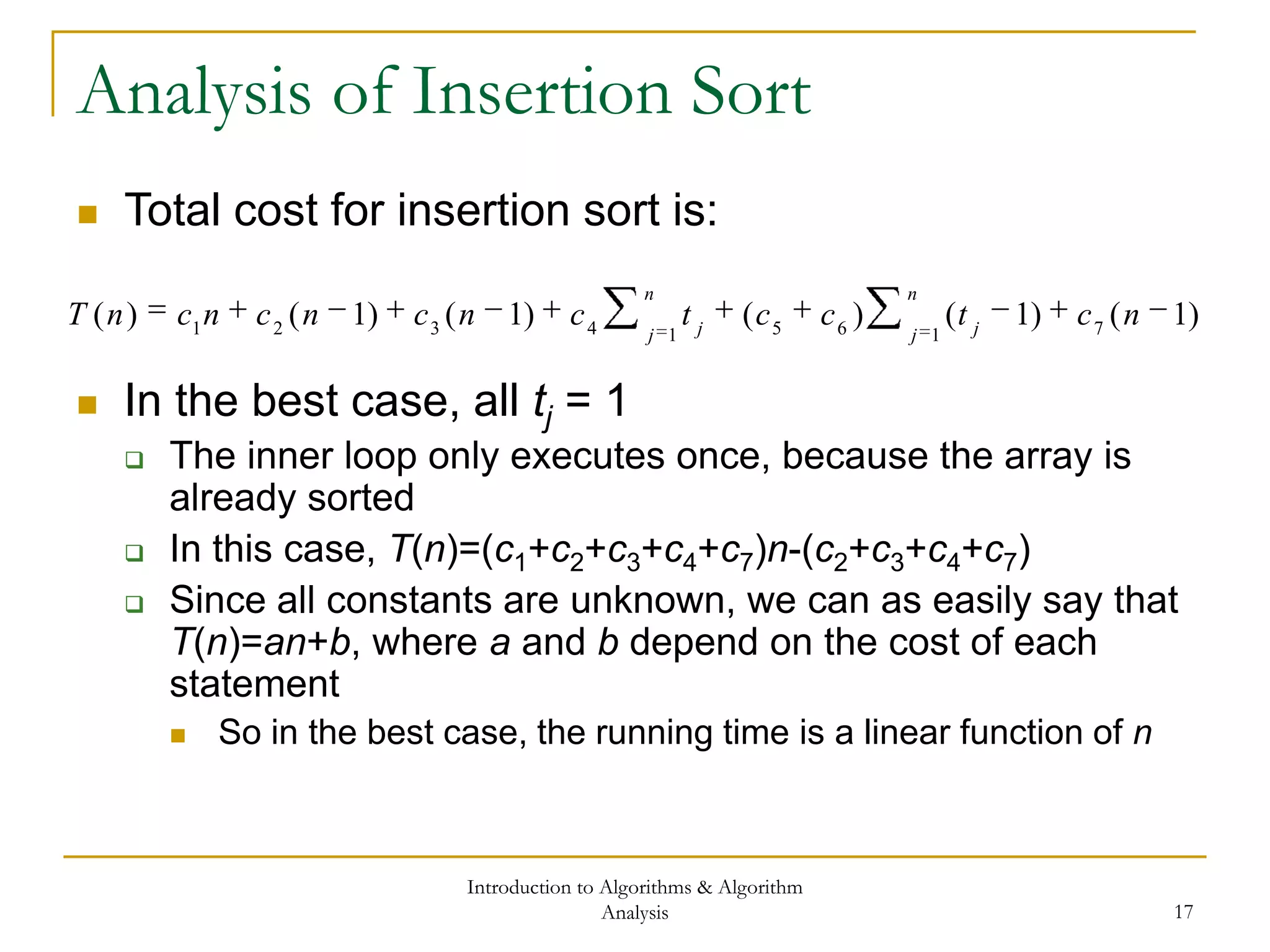
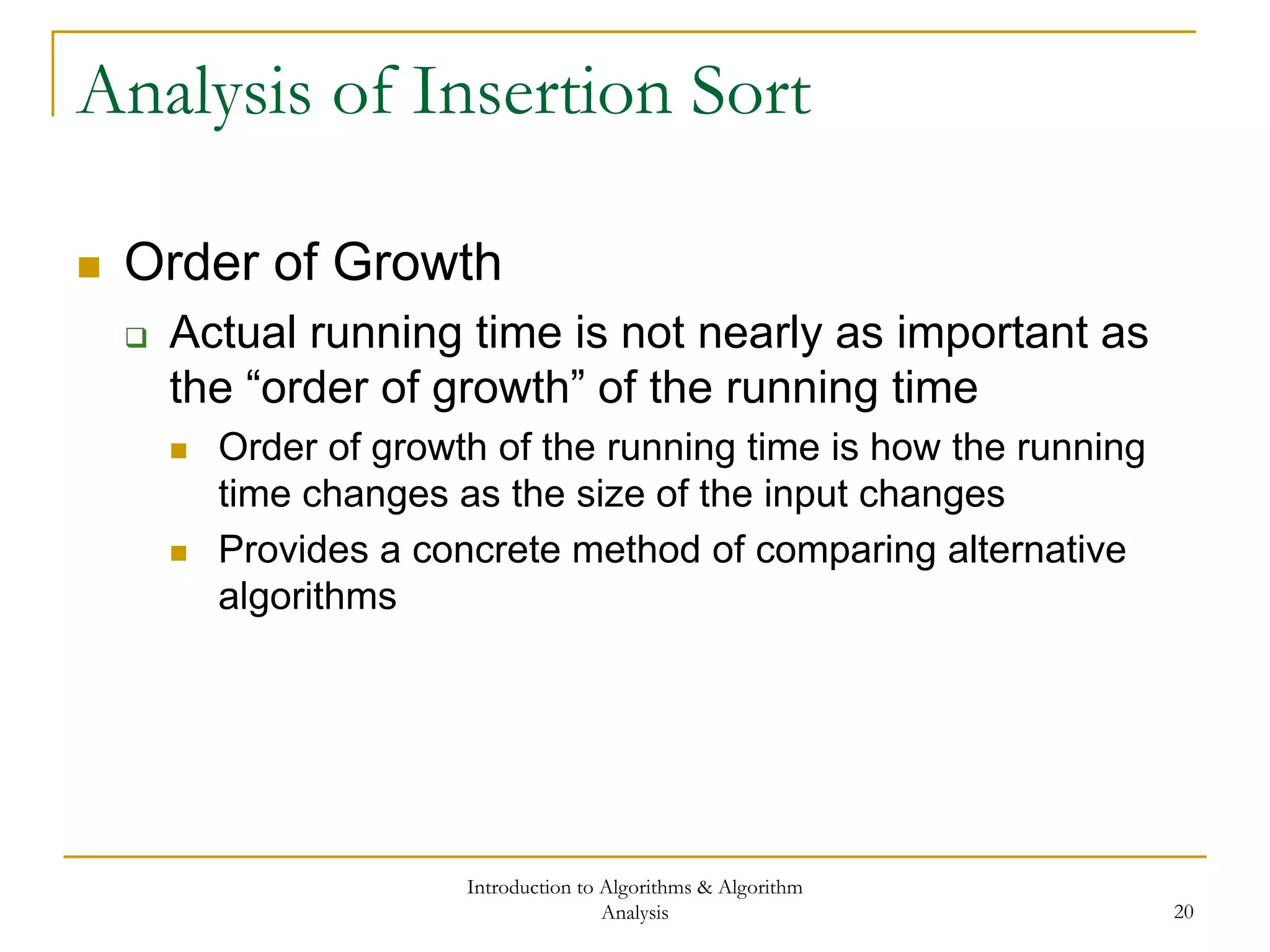
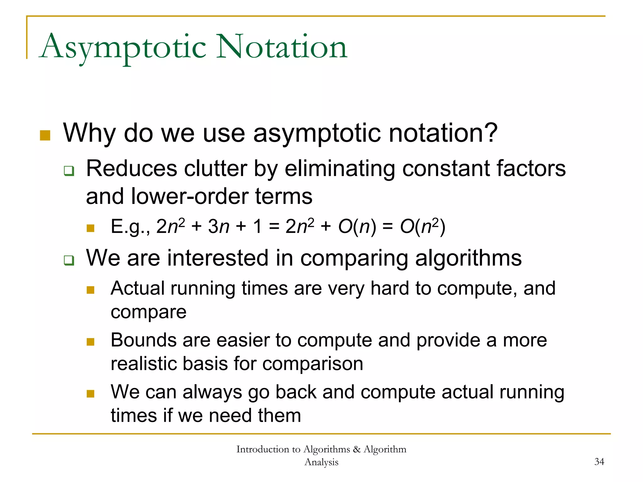
![Introduction to Algorithms & Algorithm
Analysis 16
Analysis of Insertion Sort
What is the “cost” of Insertion Sort?
Total cost = the sum of the cost of each statement *
number of times statement is executed
Statem ent Cost Tim es
for ( unsigned j = 1 ; j < size ; ++j ) c1 n
ArrayType key = A[j]; c2 n-1
int i = j-1; c3 n-1
while ( i >= 0 && A[i] > key ) c4
n
j j
t
1
A[i+1] = A[i]; c5
n
j
t j1
)1(
--i; c6
n
j
t j1
)1(
A[i+1] = key; c7 n-1](https://image.slidesharecdn.com/cis435week01-140325170012-phpapp02/75/Cis435-week01-16-2048.jpg)
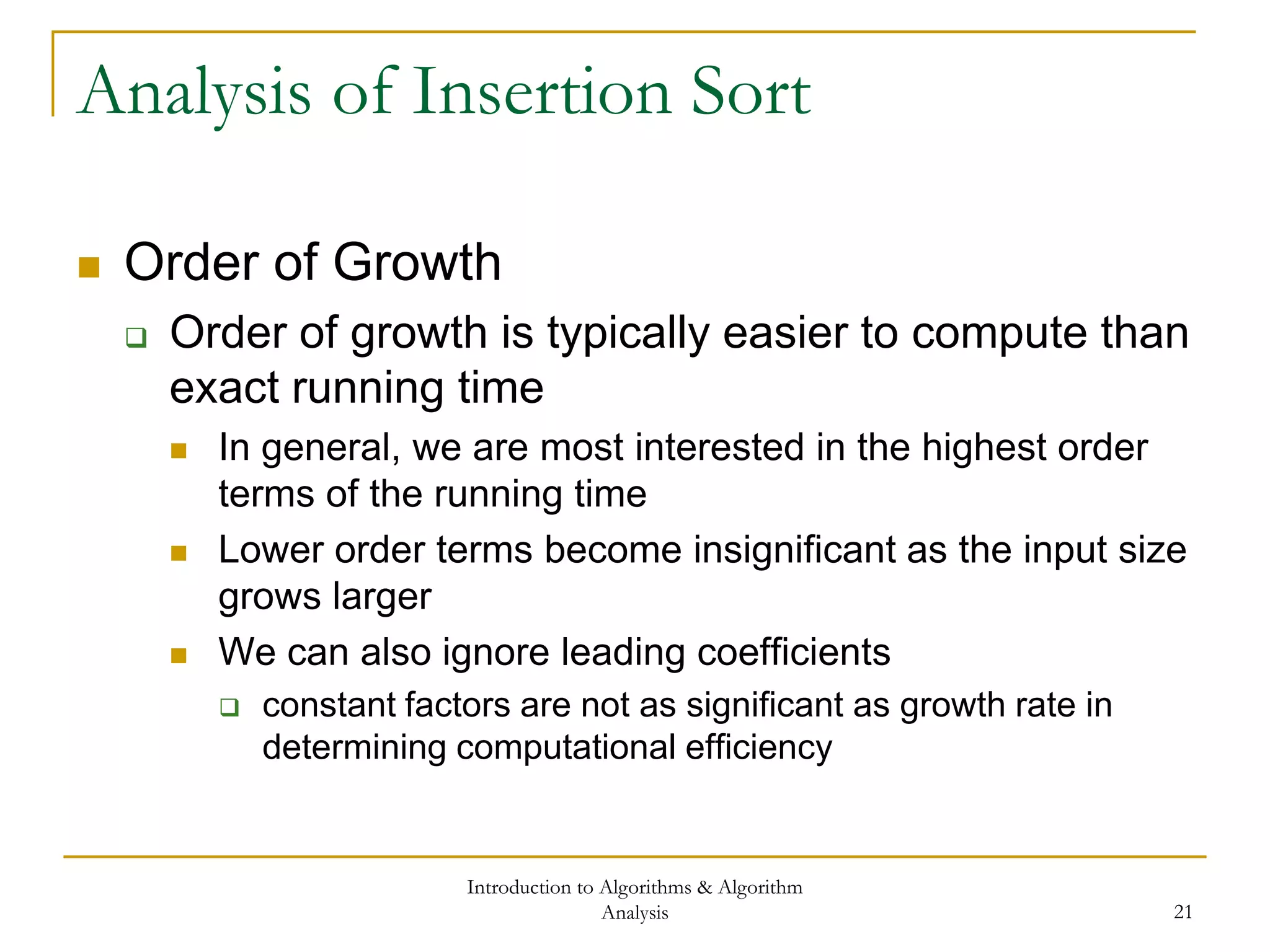
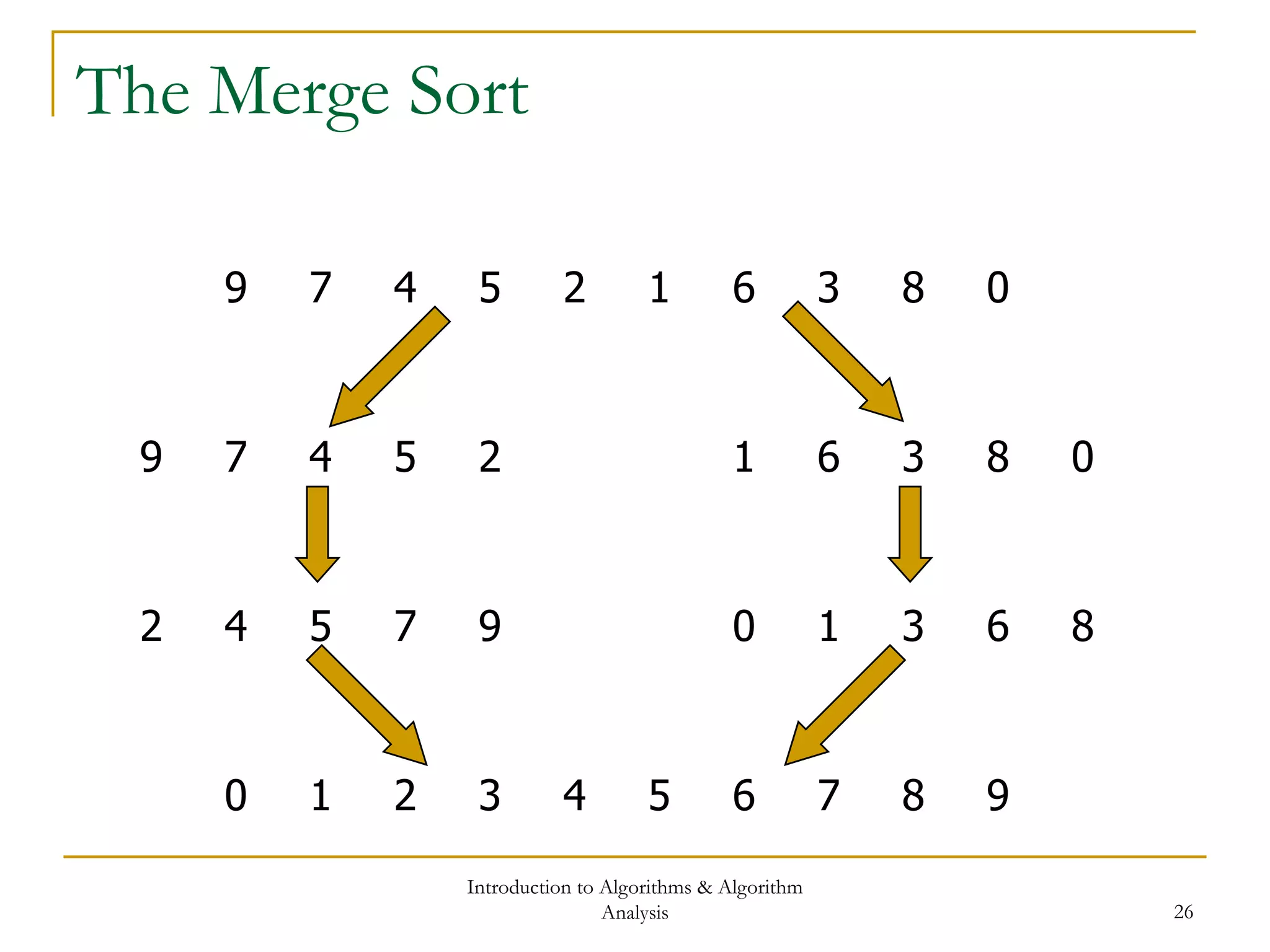
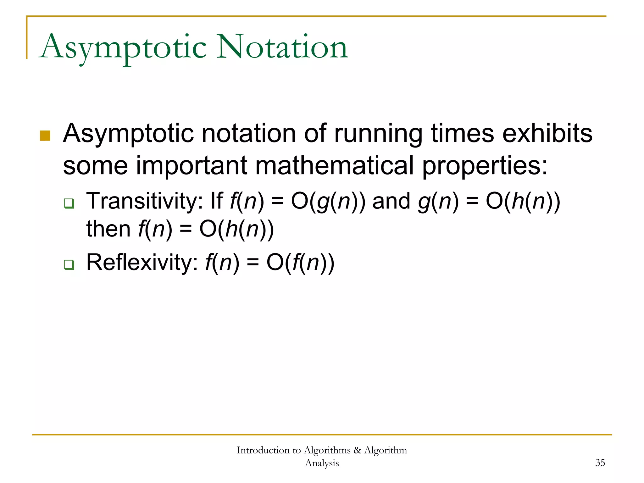
![Introduction to Algorithms & Algorithm
Analysis 27
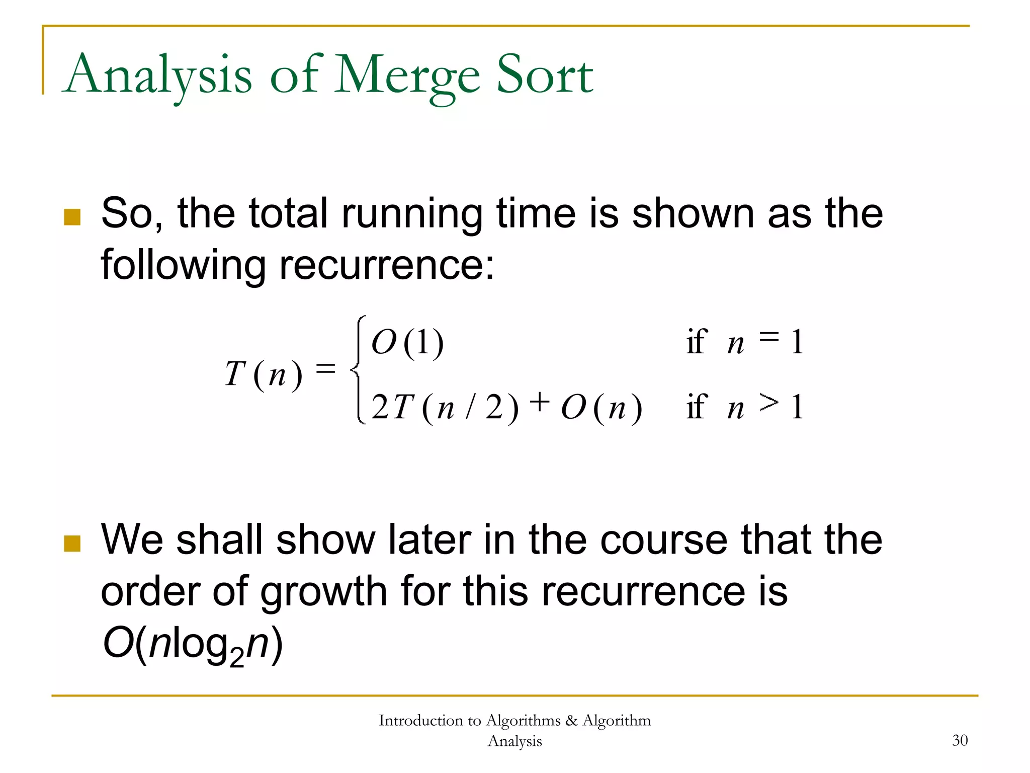
The Merge Sort
void MergeSort(ArrayType A[], int p, int r)
{
if ( p < r )
{
int q = (p+r)/2; // Divide
MergeSort(A, p, q); // Conquer left
MergeSort(A, q+1, r); // Conquer right
Merge(A, p, q, r); // Combine
}
}](https://image.slidesharecdn.com/cis435week01-140325170012-phpapp02/75/Cis435-week01-27-2048.jpg)


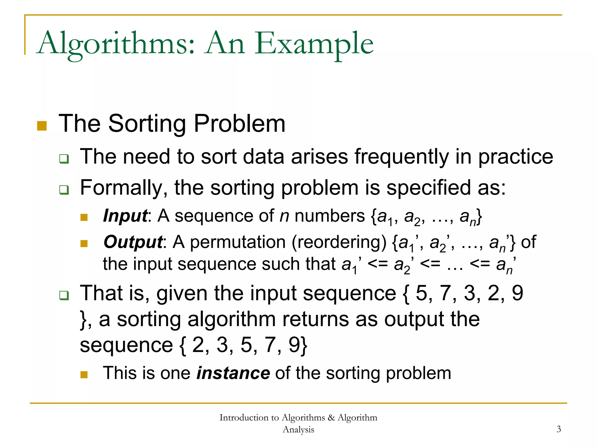
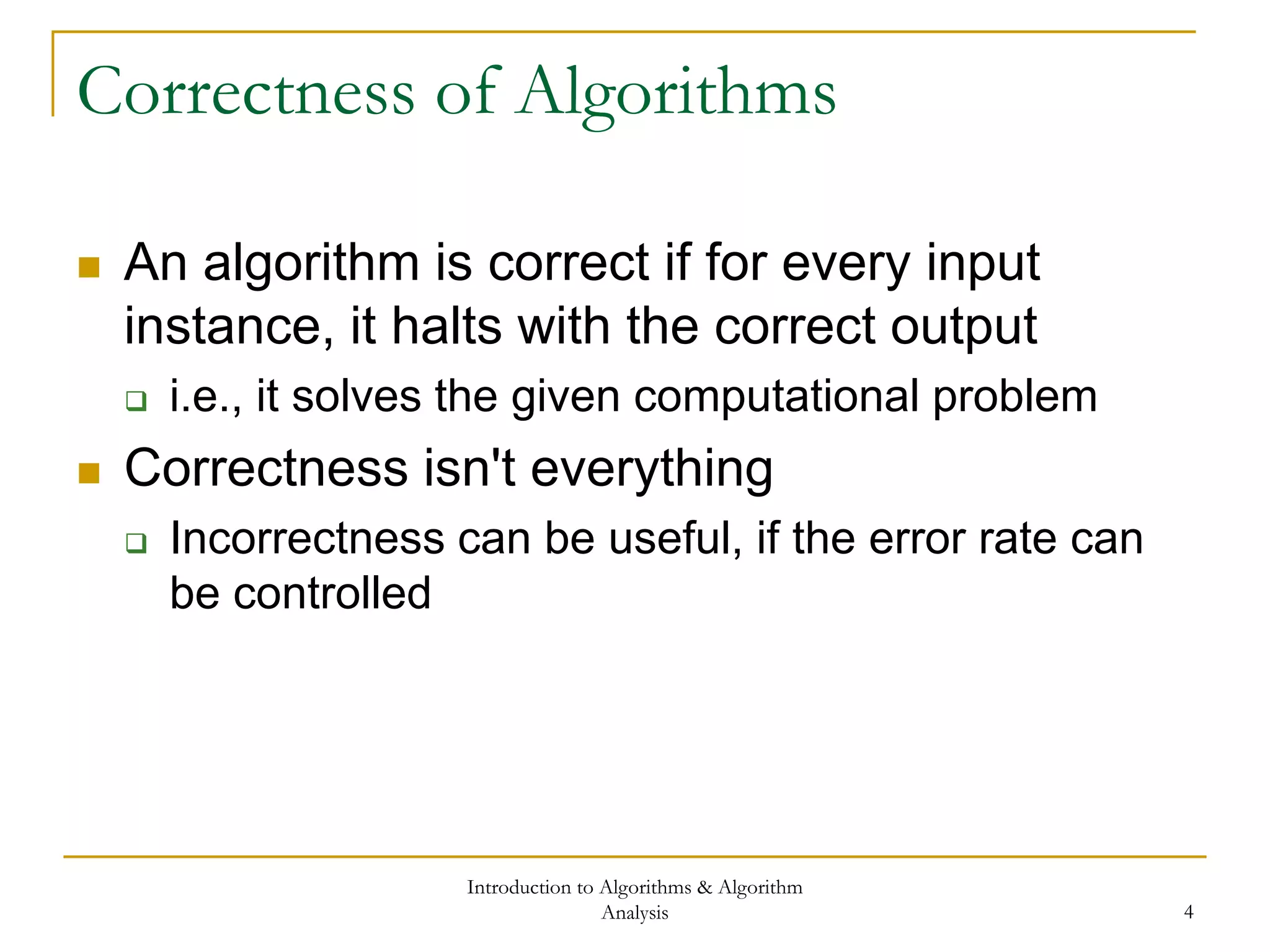
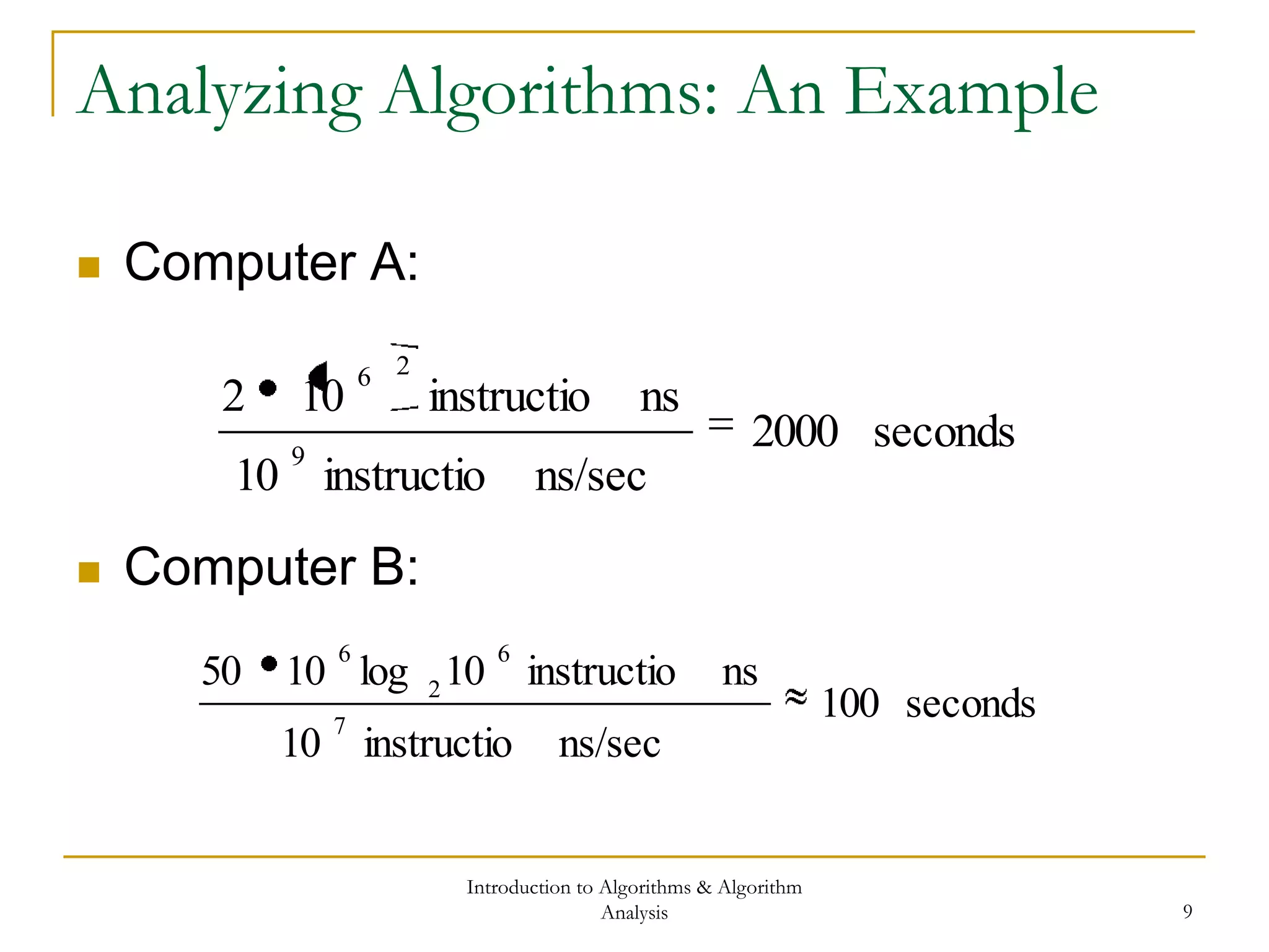
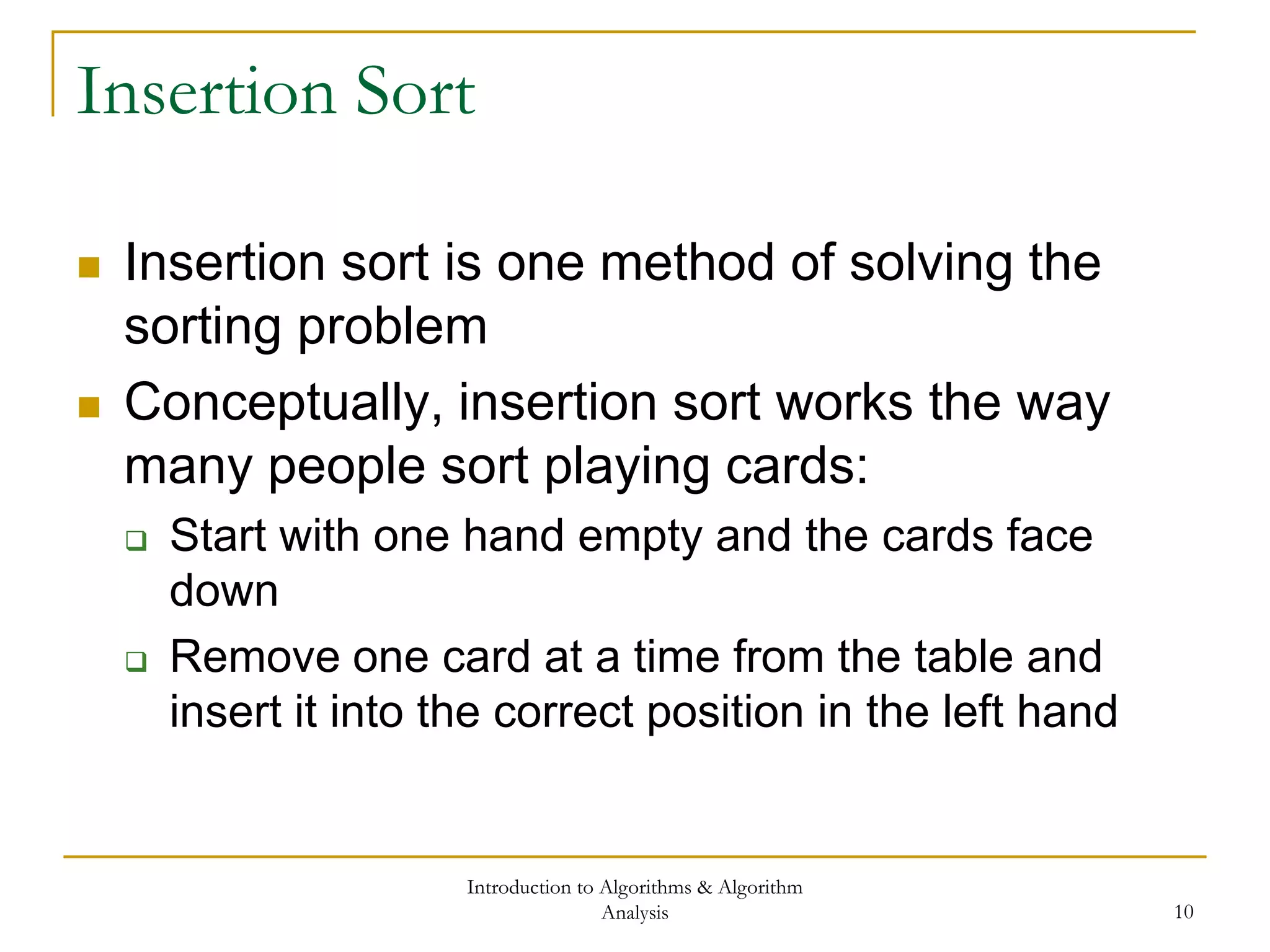
This document provides an introduction to algorithms and algorithm analysis. It defines what an algorithm is, provides examples, and discusses analyzing algorithms to determine their efficiency. Insertion sort and merge sort are presented as examples and their time complexities are analyzed. Asymptotic notation is introduced to describe an algorithm's order of growth and provide bounds on its running time. Key points covered include analyzing best-case and worst-case time complexities, using recurrences to model algorithms, and the properties of asymptotic notation. Homework problems are assigned from the textbook chapters.