Chapter 7 discusses methods for establishing causal inference in data analysis, focusing on irrelevant and proxy variables, with applications provided for each type. The chapter includes data challenges, learning objectives, and pedagogical features designed to enhance understanding and communication of analytical findings in business strategy. Additionally, it emphasizes the importance of predictive analytics in forming actionable knowledge for future managers and analysts.


![pri91516_ch03_055-082.indd 59 10/31/17 3:10 PM
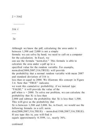
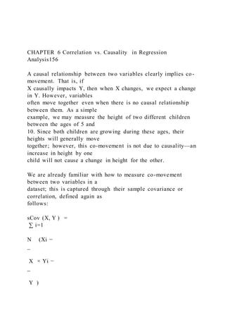
CHAPTER 3 Reasoning from Sample to Population60
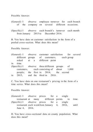
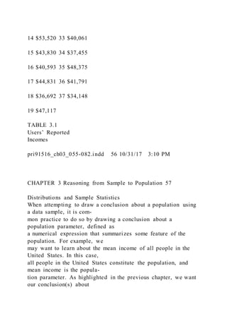
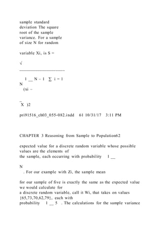
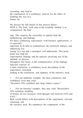
For any given distribution of a random variable, we are often
interested in two key
features—its center and its spread. Roughly speaking, we may
ask what, on average, is
the value we should expect to observe when taking a single
draw for a random variable.
And we may ask how varied (or spread out) we should expect
the observed values to be
when we take multiple draws for a random variable. A common
measure for the center of
a distribution is the expected value. We denote the expected
value of Xi (also called the
population mean) as E[Xi] and define it as the summation of
each possible realization of
Xi multiplied by the probability of that realization.
A common measure for the spread of a distribution is the
variance. We define the
variance of Xi as Var[Xi] = E[(Xi – E[Xi])
2]. Another common measure of spread is the
standard deviation. The standard deviation of Xi is si mply the
square root of the variance:
s.d.[Xi] = √
_______
Var [Xi] . As can be seen from these formulas, the variance
and standard devia-](https://image.slidesharecdn.com/chapter7-220921134402-19885515/85/Chapter-7-Basic-Methods-for-Establishing-Causal-Inference-Text-203-320.jpg)
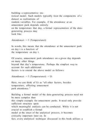
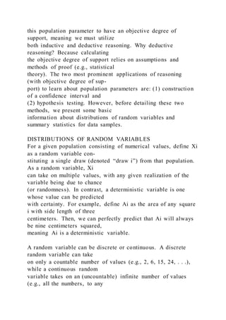
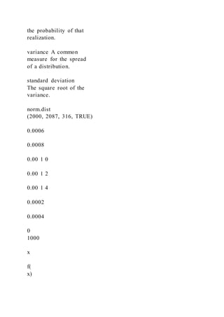
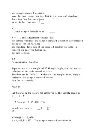
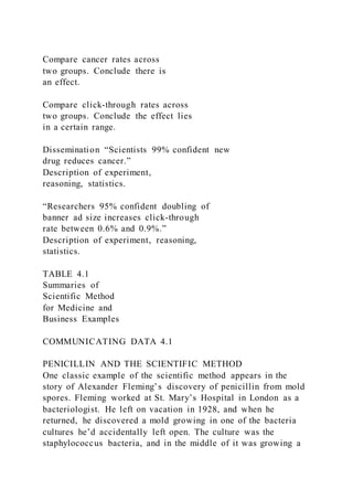
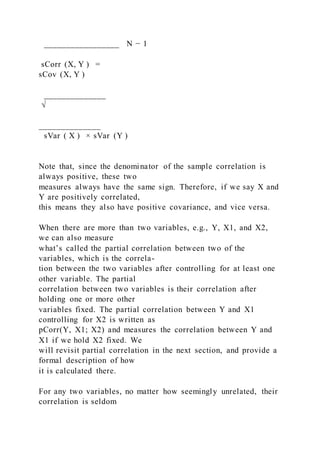
![tion are very similar measures of spread, so why do we bother
to construct both of them?
The short answer is that each plays a useful role in constructing
different statistics that are
commonly used for data analysis. The statistics we will be using
in this book generally
rely on standard deviation.
All three of the above features for a distribution—the expected
value, variance, and
standard deviation—are examples of population parameters, as
each summarizes a feature
of the population. Using our definitions, we can calculate each
parameter for our random
variables Yi and Zi. For Yi, we have:
E [Yi] = 0.3 × 25 + 0.4 × 30 + 0.2 × 40 + 0.1 × 45 = 32
Var [Yi] = 0.3 × (25 – 32)
2 + 0.4 × (30 – 32)2 + 0.2 × (40 – 32)2 + 0.1 × (45 – 32)2 = 46
s.d.[Yi] = √
__
46 = 6.78
For Zi, the calculations are analogous, but a bit more
complicated. Both the expected
value and variance involve solving integrals using the pdf (i.e.,
calculating the area
expected value
(population mean)
The summation of each
possible realization
of Xi multiplied by](https://image.slidesharecdn.com/chapter7-220921134402-19885515/85/Chapter-7-Basic-Methods-for-Establishing-Causal-Inference-Text-204-320.jpg)
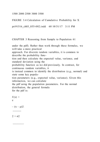
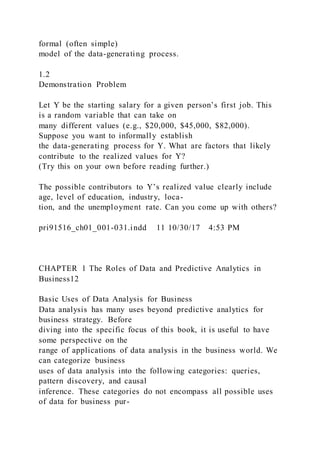
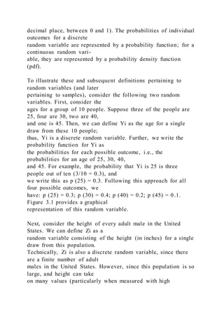
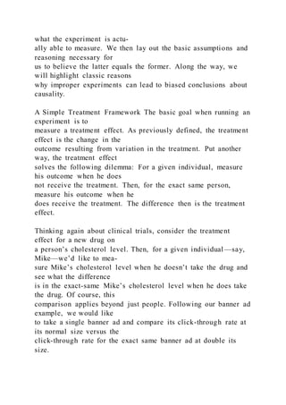
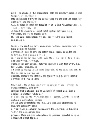
![σ √
___
2π
Here, μ is E[Xi] and σ is s.d.[Xi]. Therefore, if we specify the
expected value and stan-
dard deviation, we also know the pdf for any normal
distribution. Consequently, we often
see normal random variables represented as their distribution
type (normal), along with
their expected value and standard deviation, e.g., Xi ∼ N (μ, σ).
For Zi, the expected value
is 70 and the standard deviation is 2, and so we can write it as:
Zi ∼ N (70, 2). Using this
information, we were able to derive the pdf—f (z), which we
wrote out above—and use it
to calculate probabilities.
DATA SAMPLES AND SAMPLE STATISTICS
Now that we have described some fundamental characteristics
of distributions, we turn to
features of samples. For a random variable Xi, we define a
sample of size N as a collection of
N realizations of Xi, i.e., {x1, x2,…xN}. For example, consider
again our random variable Zi,
the height of a man in the United States, which is normally
distributed with expected value of
70 and standard deviation of 2. Suppose now we measure the
heights of five American men.
In this case, we have a sample size of five (i.e., N = 5) for the
random variable Zi. We may
represent these five measurements as a set of five numbers, e.g.,
{65,73,70,62,79}.](https://image.slidesharecdn.com/chapter7-220921134402-19885515/85/Chapter-7-Basic-Methods-for-Establishing-Causal-Inference-Text-207-320.jpg)
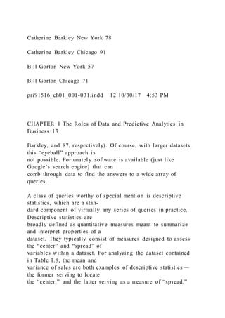
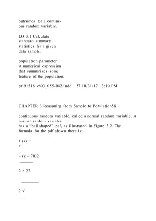
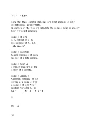
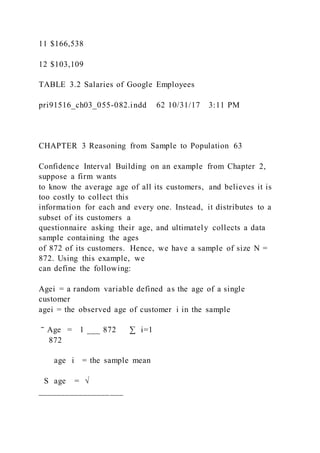
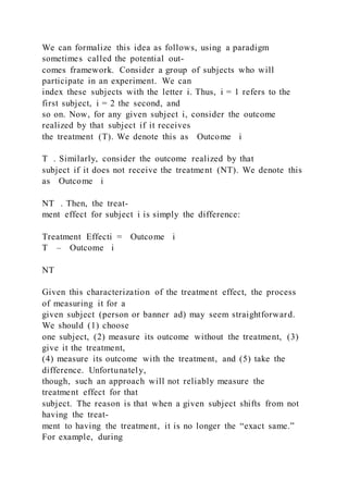
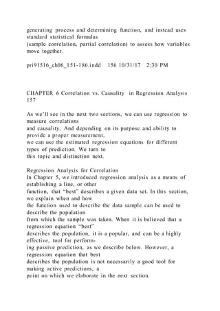
![Once we have a sample, we can calculate several sample
statistics, defined as single
measures of some feature of a data sample. As with
distributions of random variables, we
are often interested in the center and spread of a sample. A
common measure of the center
of a sample is the sample mean. The sample mean of a sample
of size N for random vari-
able Xi is X
–
= 1 __
N
[x1 + x2 + . . . + xN] =
1 __
N
∑
i = 1
N
xi. The sample mean for our sample size
of five for Zi is: Z
–
= 1 __ 5 ∑ i = 1
5
zi =
1 __ 5 [65 + 73 + 70 + 62 + 79] = 69.8.
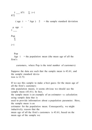
Common measures of the spread of a sample are the sample](https://image.slidesharecdn.com/chapter7-220921134402-19885515/85/Chapter-7-Basic-Methods-for-Establishing-Causal-Inference-Text-208-320.jpg)
![variance and sample
standard deviation. The sample variance of a sample of size N
for random variable Xi is
S2 = 1 __
N–1 ∑ i = 1
N
(xi – X
–
)2. The sample standard deviation of a sample of size N for ran-
dom variable Xi is the square root of the sample variance: S =
√
__________________
1 __
N – 1 ∑ i = 1
N (xi – X
–)2 .
Using our sample of size five for Zi again, we can calculate the
sample variance as
S2 = 1 __ 5 – 1 ∑ i = 1
5
(zi – Z
–
)2 = 1 __ 4 . [65 – 69.8)
2 + . . . + (79 – 69.8)2] = 44.7. Also, the sample
standard deviation for this sample is √](https://image.slidesharecdn.com/chapter7-220921134402-19885515/85/Chapter-7-Basic-Methods-for-Establishing-Causal-Inference-Text-209-320.jpg)


![and identically
distributed (i.i.d)
The distribution of one
random variable does
not depend on the
realization of another
and each has identical
distribution.
pri91516_ch03_055-082.indd 64 10/31/17 3:11 PM
CHAPTER 3 Reasoning from Sample to Population 65
Still assuming a random sample, it can be shown that the mean
of X ̅ (that is, the mean
of the sample mean) is the population mean, μ. Mathematically,
we have: E [ X ̅ ] = μ . Rather
than provide a formal proof, consider the following intuition.
Let Xi be the weight of an
adult American, and suppose we weigh two Americans. Hence,
we observe a value for X1
and X2. Suppose we knew E[Xi] = 180 pounds. In words, we
know the mean weight of all
American adults is 180 pounds. If we then randomly pick and
weigh two American adults,
and average their weights, what should we expect that average
to be? If, on average, the
first measurement is 180 and the second measurement is 180,
then we should expect the
average of these two measures to be 180 (i.e., 180 + 180
_______ 2 = 180).
An estimator whose mean is equal to the population parameter it
is used to estimate is](https://image.slidesharecdn.com/chapter7-220921134402-19885515/85/Chapter-7-Basic-Methods-for-Establishing-Causal-Inference-Text-221-320.jpg)
![known as an unbiased estimator. Since the mean of X ̅ is
equal to the population mean,
we say that the sample mean is an unbiased estimator for the
population mean. This justi-
fies using the sample mean as a “best guess” for the population
mean and the center for
any confidence interval we will use. One could also formally
show that the mean of the
sample variance is the variance you would calculate if you
collected the entire population,
i.e., the population variance formally, ( E [ S 2 ] = σ 2 ). In
addition, the mean of the sample
standard deviation is the population standard deviation, the
square root of the population
variance formally, ( E [S] = σ ) . Hence, each sample measure
is an unbiased estimator of
its population counterpart.
In order to construct a confidence interval for the population
mean and know its objec-
tive degree of support, we must learn more about the
distribution of the sample mean
beyond just its expected value. In particular, we must know
something about its standard
deviation and its type of distribution. Regarding the former, the
assumption that a data
sample is a random sample implies the standard deviation of the
sample mean is σ __
√
__
N
.
More succinctly, we have: s . d. [ X ̅ ] = σ __](https://image.slidesharecdn.com/chapter7-220921134402-19885515/85/Chapter-7-Basic-Methods-for-Establishing-Causal-Inference-Text-222-320.jpg)


![The above cutoffs are worth committing to memory. However, it
is useful to note that they
are reasonably close to cutoffs of 1.5, 2, and 2.5, respectively.
Although these rougher
cutoff values are less precise and should not be used in general,
they can be helpful when
quickly and roughly assessing statistical outputs if the more
precise cutoffs do not imme-
diately come to mind.
Since the sample mean is normally distributed when there is a
large, random sample,
the above probabilities apply. We can write these probabilities
more formally and suc-
cinctly for the sample mean as follows.
For a random data sample of size N > 30,
Pr ( X ̅ ∈ [μ ± 1.65 (
σ __
√
__
N
) ] ) ≈ 0.9
Pr ( X ̅ ∈ [μ ± 1.96 (
σ __
√
__
N
) ] ) ≈ 0.95](https://image.slidesharecdn.com/chapter7-220921134402-19885515/85/Chapter-7-Basic-Methods-for-Establishing-Causal-Inference-Text-226-320.jpg)
![Pr ( X ̅ ∈ [μ ± 2.58 (
σ __
√
__
N
) ] ) ≈ 0.99
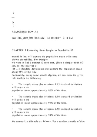
This idea is illustrated in Figure 3.5 for the case of 95%
probability. (For 90%, the range is
narrower, and for 99% the range is wider.)
For the above probabilities, we are taking the population mean
and creating an interval
around it to capture a certain percentage (e.g., 90%, 95%) of all
possible draws for the
sample mean. For example, we have that, given a population
mean of, say, 10, the sample
mean will fall within 1.96 standard deviations of 10 about 95%
of the time.
Although we now have substantial information about the sample
mean, our objective is
not to predict where the sample mean will fall; we observe the
sample mean when we col-
lect a data sample. Instead, we want to take an observed sample
mean and create an interval
THE DISTRIBUTION OF THE SAMPLE MEAN
If a sample of size N is a random sample and N is “large” (>
30), then X ̅ ∼ N (μ,
σ __](https://image.slidesharecdn.com/chapter7-220921134402-19885515/85/Chapter-7-Basic-Methods-for-Establishing-Causal-Inference-Text-227-320.jpg)
![N > 30,
Pr (μ ∈ [ X ̅ ± 1.65 (
σ __
√
__
N
) ] ) ≈ 0.9
Pr (μ ∈ [ X ̅ ± 1.96 (
σ __
√
__
N
) ] ) ≈ 0.95
Pr (μ ∈ [ X ̅ ± 2.58 (
σ __
√
__
N
) ] ) ≈ 0.99
At this point, we now have formulas for confidence intervals
that have objective degrees of
support. For example, if we take the sample mean and then add
and subtract 1.96 standard
deviations, we know this will contain the population mean
approximately 95% of the time.
Or, put another way, we are 95% confident this interval will](https://image.slidesharecdn.com/chapter7-220921134402-19885515/85/Chapter-7-Basic-Methods-for-Establishing-Causal-Inference-Text-229-320.jpg)
![pri91516_ch03_055-082.indd 67 10/31/17 3:11 PM
CHAPTER 3 Reasoning from Sample to Population68
looks like a normal distribution but requires larger numbers of
standard deviations to
achieve the same probabilities as the normal distribution (e.g.,
2, 2.5, and 4 standard
deviations might be necessary to attain 90%, 95%, and 99%
probabilities, respectively).
However, when N > 30 (which we already are assuming in order
to apply the central limit
theorem), the difference between a t-distribution and normal
distribution becomes trivial,
and so the same probability formulas apply. Consequently, the
confidence interval formu-
las become as follows. For a random sample of size N > 30,
Pr (μ ∈ [ X ̅ ± 1.65 (
S __
√
__
N
) ] ) ≈ 0.9
Pr (μ ∈ [ X ̅ ± 1.96 (
S __
√
__](https://image.slidesharecdn.com/chapter7-220921134402-19885515/85/Chapter-7-Basic-Methods-for-Establishing-Causal-Inference-Text-231-320.jpg)
![N
) ] ) ≈ 0.95
Pr (μ ∈ [ X ̅ ± 2.58 (
S __
√
__
N
) ] ) ≈ 0.99
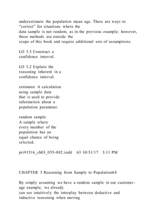
Revisiting our initial example involving mean customer ages,
we can construct all three
confidence intervals immediately using the provided sample
information. Therefore, using
the sample mean of 43.61, sample standard deviation of 12.72,
and sample size of 872,
we have the following confidence intervals for the mean age of
all the firm’s customers:
90% confidence interval: (43.61 ± 1.65 ( 12.72 _____ √ ____
872 ) ) = (42.90, 44.32)
95% confidence interval: (43.61 ± 1.96 ( 12.72 _____ √ ____
872 ) ) = (42.77, 44.45)
99% confidence interval: (43.61 ± 2.58 ( 12.72 _____ √ ____
872 ) ) = (42.50, 44.72)
We summarize the reasoning associated with confidence
intervals in Reasoning Box 3.2.
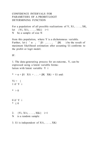
CONFIDENCE INTERVALS
Deductive reasoning:
IF:](https://image.slidesharecdn.com/chapter7-220921134402-19885515/85/Chapter-7-Basic-Methods-for-Establishing-Causal-Inference-Text-232-320.jpg)

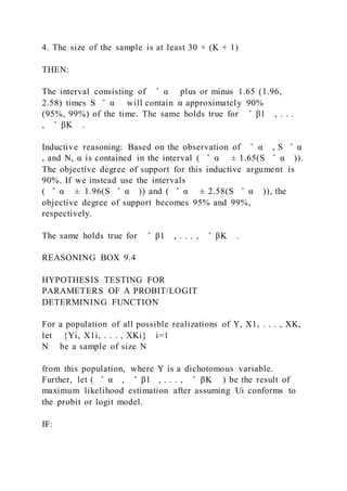
![THE DISTRIBUTION OF THE SAMPLE MEAN
FOR HYPOTHESIZED POPULATION MEAN
REASONING BOX 3.3
If a sample of size N is a random sample, N is “large” (> 30),
and μ = K, then X ̅ ∼ N (K,
σ __
√
__
N
) .
pri91516_ch03_055-082.indd 71 10/31/17 3:11 PM
CHAPTER 3 Reasoning from Sample to Population72
For a random data sample of size N > 30, and population mean
= K,
Pr ( X ̅ ∈ [K ± 1.65 (
σ __
√
__
N
) ] ) ≈ 0.9
Pr ( X ̅ ∈ [K ± 1.96 (
σ __](https://image.slidesharecdn.com/chapter7-220921134402-19885515/85/Chapter-7-Basic-Methods-for-Establishing-Causal-Inference-Text-242-320.jpg)
![√
__
N
) ] ) ≈ 0.95
Pr ( X ̅ ∈ [K ± 2.58 (
σ __
√
__
N
) ] ) ≈ 0.99
This idea is illustrated in Figure 3.6 for the case of 95%. In
contrast to Figure 3.5, the
sample mean centers on an assumed value of K, rather than an
unknown value of μ.
Notice that, by assuming our null hypothesis along with a large
random sample, we
have arrived at an empirically testable conclusion, i.e., a
random variable with known
distribution and consequently known probabilities for various
outcomes. In fact, hypoth-
esis tests fall exactly into the reasoning framework described in
Chapter 2 for evaluating
assumptions. Here, the null hypothesis is the assumption we
would like to evaluate. Recall
that the general process for evaluating assumptions is to: (1)
Use deductive reasoning to
arrive at an empirically testable conclusion, (2) Collect a data
sample and use inductive
reasoning to decide whether or not to reject the empirically](https://image.slidesharecdn.com/chapter7-220921134402-19885515/85/Chapter-7-Basic-Methods-for-Establishing-Causal-Inference-Text-243-320.jpg)


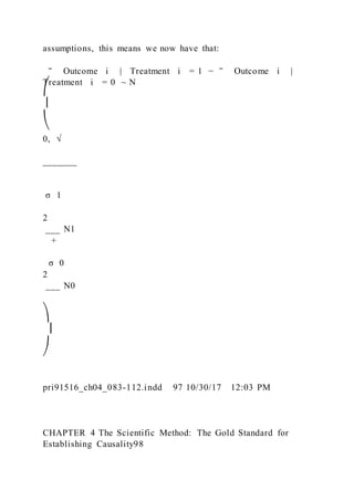
![treatment effect for a
randomly drawn subject from the population, written as
E[Treatment Effecti]. Expanding
on this, we have:
ATE = E [Treatment Effecti] = E [ Outcome i
T – Outcome i
NT ]
With the estimation of the ATE for a given treatment as our
objective, we now turn to how
experiments can help up accomplish this goal.
From Experiments to Treatment Effects How can an experiment
provide us with an
estimate of the average treatment effect? The answer to this
question is best understood by
considering an experiment with a dichotomous treatment—that
is, a treatment in which
participants are split into two groups where one receives the
treatment (takes a drug) and
the other does not (takes a placebo).
To begin, we define two more variables, whose values are
determined by the experi-
ment. The first is a dichotomous variable, Treatedi. This
variable equals 1 if subject i actu-
average treatment
effect (ATE) The
average difference in the
treated and untreated
outcome across all sub-
jects in a population.](https://image.slidesharecdn.com/chapter7-220921134402-19885515/85/Chapter-7-Basic-Methods-for-Establishing-Causal-Inference-Text-292-320.jpg)
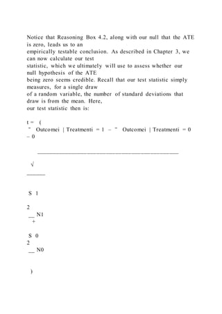
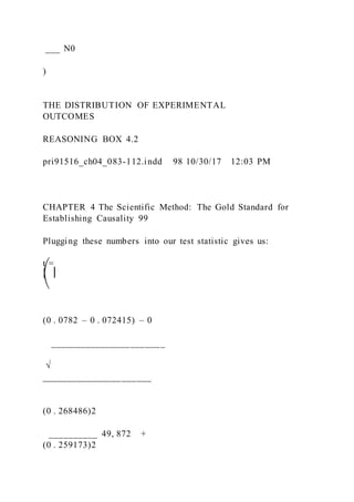
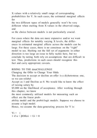
![then we may conclude the ATE = –18 – (–3) = –15.
However, would we arrive at such a conclusion if we were told
all of the subjects were
men? Or, what if the drug were administered only to people
weighing over 230 pounds?
If either case were true, we may have serious doubt as to
whether –15 is a good estimate
of the true ATE. The key question then emerges: When does the
difference in the mean
outcomes across the treated and untreated groups yield an
unbiased estimate of the ATE?
Or, when does the following relationship hold?
E [ ‾ Outcomei | Treatedi = 1 – ‾ Outcomei | Treatedi = 0
] = ATE
We propose that this relationship holds for a given experiment
when two conditions are
satisfied by that experiment:
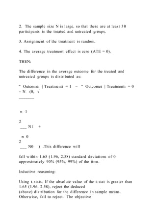
1. Participants are a random sample of the population.
2. Assignment into the treated group is random.
As we showed in Chapter 3, if participants are a random sample
of the population, then
means for the data sample are unbiased estimators for their
population counterparts. This
relationship is true for conditional means as well. Thus, in our
case, we have:
E [ ‾ Outcomei | Treatedi = 1 ] = E [Outcomei | Treatedi = 1]
pri91516_ch04_083-112.indd 91 10/30/17 12:03 PM](https://image.slidesharecdn.com/chapter7-220921134402-19885515/85/Chapter-7-Basic-Methods-for-Establishing-Causal-Inference-Text-295-320.jpg)
![CHAPTER 4 The Scientific Method: The Gold Standard for
Establishing Causality92
and
E [ ‾ Outcomei | Treatedi = 0 ] = E [Outcomei | Treatedi = 0].
In words, the mean outcomes for those assigned the treatment
and those that weren’t
in the experiment are unbiased estimates of the mean outcomes
in the population
for those that would have received the treatment and those that
wouldn’t. Hence, our
first condition is straightforward. It ensures that the sample
averages we collect are
good estimates of the population parameters to which they
naturally correspond. It
also leads to the following result: If participants are a random
sample of the popula-
tion, then
E [ ‾ Outcomei | Treatedi = 1 – ‾ Outcomei | Treatedi = 0 ]
=
E [Outcomei | Treatedi = 1] – E [Outcomei | Treatedi = 0]
That is, the expected difference in the mean outcome for the
treated and untreated groups
(top part) equals the difference in the mean outcome in the
population between those that
would have received the treatment and those that wouldn’t
(bottom part).
Based on our result from condition #1, we now just need
condition #2 to ensure that
E [Outcomei | Treatedi = 1] – E[Outcomei | Treatedi = 0] = ATE](https://image.slidesharecdn.com/chapter7-220921134402-19885515/85/Chapter-7-Basic-Methods-for-Establishing-Causal-Inference-Text-296-320.jpg)
![in order for the two con-
ditions to imply E [ ‾ Outcomei | Treatedi = 1 – ‾ Outcomei
| Treatedi = 0 ] = ATE. In other
words, we need random treatment assignment to ensure that the
difference in expected
outcome between those who are treated and untreated equals the
expected difference in
outcome when a given individual goes from being untreated to
treated (ATE).
To assess whether this is the case, let’s consider reasons why
the mean outcome for
those who received the treatment might differ from the mean
outcome for those who did
not receive the treatment. In fact, there are two reasons this
might be the case. First, those
receiving the treatment may respond to it; that is, there is a non-
zero average treatment effect
at least for the group who were given the treatment. This non-
zero average treatment effect
for the group given the treatment is called the effect of the
treatment on the treated (ETT).
Using our notation, and this definition, we have:
ETT = E [ Outcome i T – Outcome i NT | Treatedi = 1]
If an ETT exists, then even if both groups have the same mean
outcome when not given
the treatment, a difference emerges once the group chosen to get
the treatment receives it.
Second, the treated and untreated groups may be starting from
different places. In par-
ticular, the mean outcome for the treated group may be different
from the mean outcome for
the untreated group, even if neither actually received the](https://image.slidesharecdn.com/chapter7-220921134402-19885515/85/Chapter-7-Basic-Methods-for-Establishing-Causal-Inference-Text-297-320.jpg)
![treatment. In such a situation, we
say there is a selection bias in the experiment. Again using our
notation and this definition,
we have: Selection Bias = E [ Outcome i
NT | Treatedi = 1] – E [ Outcome i
NT | Treatedi = 0].
If a selection bias exists, then even if the treated group showed
no response to the treat-
ment, their mean outcomes would differ due to differences in
their mean outcomes before
any treatment was received.
To further illustrate these points, consider again our experiment
with the cholesterol
drug. Suppose we have 500 subjects who receive the drug and
500 subjects who do not
receive the drug. Suppose again that the average change in
cholesterol level for those who
took the drug was –18, and the average change in cholesterol
level for those who did not
effect of the treat-
ment on the treated
(ETT) Average treat-
ment effect for the group
given the treatment.
selection bias The
mean outcome for the
treated group would
differ from the mean out-
come for the untreated
group in the case where
neither receives the](https://image.slidesharecdn.com/chapter7-220921134402-19885515/85/Chapter-7-Basic-Methods-for-Establishing-Causal-Inference-Text-298-320.jpg)
![ETT and selection bias. For example, the drug may lower
cholesterol by 7 for the treated
group, and their cholesterol would have gone down by 11 even
without the drug. In that
case, the ETT is –7, and selection bias is –8 (–11 – (–3)).
We can now express the difference in mean outcomes for treated
and untreated subjects
as follows:
E [Outcomei ∣ Treatedi = 1] – E [Outcomei ∣ Treatedi = 0] =
ETT + Selection Bias
Consequently, we must determine whether random treatment
assignment implies ETT +
Selection Bias = ATE. To answer this question, we highlight the
key implication of ran-
dom treatment assignment. If treatment is assigned randomly,
then the group to which a
participant is assigned will provide no information about (1)
how he responds to the treat-
ment, or (2) his outcome if he were not to get the treatment. To
make this more concrete,
suppose group assignment for our cholesterol example is
determined by the flip of a coin,
and all those who land heads get the treatment and those who
land tails do not. Under such
a system, should we expect those who land heads to respond to
the treatment differently?
Or, should we expect those who land heads to have different
untreated cholesterol levels
than those who land tails? The answer to both questions is
certainly “No.” The result of a
coin toss has nothing to do with either of these measures.
Let’s now consider the implication of random treatment](https://image.slidesharecdn.com/chapter7-220921134402-19885515/85/Chapter-7-Basic-Methods-for-Establishing-Causal-Inference-Text-300-320.jpg)
![assignment for ETT and
Selection Bias in turn. To begin, we know ETT = E [ Outcome
i
T – Outcome i
NT | Treatedi = 1].
However, with random treatment assignment, we know
assignment to the treatment group
provides no information about a subject’s response to the
treatment. Hence, conditioning
on group assignment is completely uninformative, and so we
have:
ETT = E [ Outcome i T – Outcome i NT | Treatedi = 1] =
E [ Outcome i T – Outcome i NT ] = ATE
That is, with random treatment assignment, the effect of the
treatment on the treated is
equal to the average treatment effect.
Next, recall that:
Selection Bias = E [ Outcome i
NT | Treatedi = 1] – E [ Outcome i NT | Treatedi = 0]
Again, with random treatment assignment, we know assignment
to either group (treated
or untreated) provides no information about a subject’s outcome
were he not to receive
pri91516_ch04_083-112.indd 93 10/30/17 12:03 PM
CHAPTER 4 The Scientific Method: The Gold Standard for](https://image.slidesharecdn.com/chapter7-220921134402-19885515/85/Chapter-7-Basic-Methods-for-Establishing-Causal-Inference-Text-301-320.jpg)
![Establishing Causality94
the treatment. Consequently, it is again the case that
conditioning on group assignment is
completely uninformative, meaning we have:
Selection Bias = E [ Outcome i
NT | Treatedi = 1] – E [ Outcome i NT | Treatedi = 0]
= E [ Outcome i
NT ] – E [ Outcome i NT ] = 0
In short, random treatment assignment means there is not
selection bias. Putting both of
these results together, we have that ETT + Selection Bias =
ATE + 0 = ATE.
In Reasoning Box 4.1, we detail the reasoning that leads us
from an experiment to ulti-
mately measuring a treatment effect.
THE TREATMENT EFFECT
If experiment participants are a random sample from the
population and the treatment is randomly
assigned, then the difference in the mean outcomes for the
treated group and untreated group is an
unbiased estimate of the average treatment effect.
REASONING BOX 4.1
4.1
Demonstration Problem
Suppose a grocery store is interested in learning the effect of
promoting (via a standing sign) a candy](https://image.slidesharecdn.com/chapter7-220921134402-19885515/85/Chapter-7-Basic-Methods-for-Establishing-Causal-Inference-Text-302-320.jpg)


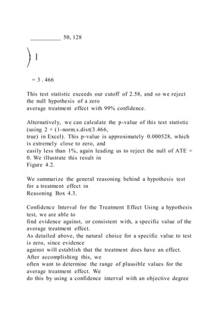
![H0: Changing an ad’s placement from fourth to first position
has (on average)
no impact on click-through rates.
If we define the incidence of a click (= 0 or 1) as the outcome
and the movement of an
ad from fourth to first position as the treatment, then we have
the standard null hypothesis
when testing for a treatment effect, namely, that the average
treatment effect is zero:
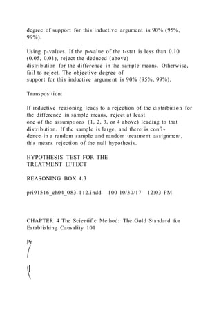
H0: ATE = E [ Outcome i T – Outcome i NT ] = 0
The data from our experiment will provide us with the average
incidence of a click
(the click-through rate) for ads in top position and the click-
through rate for ads
in fourth position. Hence, the data provide us with ‾
Outcomei | Treatmenti = 1 and
‾ Outcomei | Treatmenti = 0 .
Following Reasoning Box 3.1, we know that, for a large,
random sample (as we have
here), these sample means have the following distributions:
‾ Outcomei | Treatmenti = 1 ~ N (
μ1,
σ1 ____
√
___
N1
)](https://image.slidesharecdn.com/chapter7-220921134402-19885515/85/Chapter-7-Basic-Methods-for-Establishing-Causal-Inference-Text-310-320.jpg)
![‾ Outcomei | Treatmenti = 0 ~ N (
μ0,
σ0 ____
√
___
N0
)
Here we define: μ1 = E [Outcomei | Treatmenti = 1], μ0 = E
[Outcomei | Treatmenti = 0],
σ1 = √
__________________________
Var [Outcomei | Treatmenti = 1] , σ0 = √
__________________________
Var [Outcomei | Treatmenti = 0] , N1 = the
number of treated observations, and N0 = the number of
untreated observations.
A well-known property in statistics is that the sum, or
difference, of normal random variables
is also a normal random variable—adding or subtracting does
not change the shape of the dis-
tribution. As a result, we know that the difference in the click-
through rates between the treated
and untreated observations is normally distributed, since each
click-through rate is normally dis-
tributed. Using this fact along with basic formulas for expected](https://image.slidesharecdn.com/chapter7-220921134402-19885515/85/Chapter-7-Basic-Methods-for-Establishing-Causal-Inference-Text-311-320.jpg)
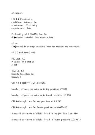
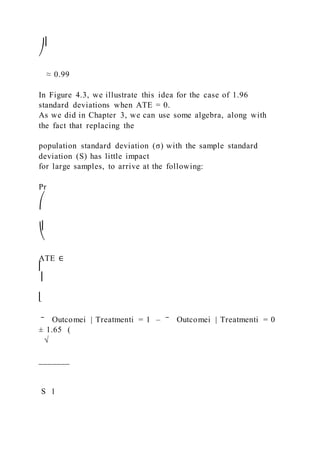
![value and variance, we now have:
‾ Outcomei | Treatmenti = 1 – ‾ Outcomei | Treatmenti =
0 ~ N
⎛
⎜
⎝
μ1 – μ0, √
_______
σ 1
2
___
N1
+
σ 0
2
___
N0
⎞
⎟
⎠
Lastly, as we proved earlier in this chapter, we know that
random treatment assignment
implies E [Outcomei ∣ Treatmenti = 1] – E [Outcomei ∣](https://image.slidesharecdn.com/chapter7-220921134402-19885515/85/Chapter-7-Basic-Methods-for-Establishing-Causal-Inference-Text-312-320.jpg)
![Treatmenti = 0] = ATE. Thus, given
our definitions for μ1 and μ0, we have μ1 – μ0 = ATE and
‾ Outcomei | Treatmenti = 1 – ‾ Outcomei | Treatmenti =
0 ~ N
⎛
⎜
⎝
ATE, √
_______
σ 1
2
___
N1
+
σ 0
2
___
N0
⎞
⎟
⎠
Following Reasoning Box 4.2, if we add our null hypothesis
that ATE = 0 to our set of](https://image.slidesharecdn.com/chapter7-220921134402-19885515/85/Chapter-7-Basic-Methods-for-Establishing-Causal-Inference-Text-313-320.jpg)


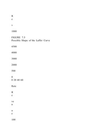
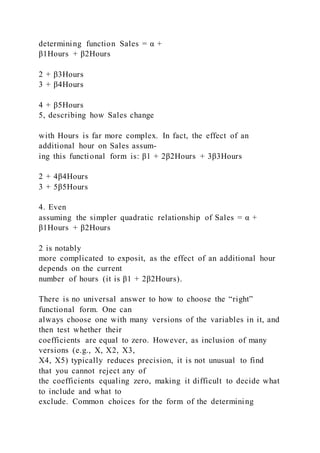
![and Sales
pri91516_ch04_083-112.indd 106 10/30/17 12:03 PM
CHAPTER 4 The Scientific Method: The Gold Standard for
Establishing Causality 107
CONSEQUENCES OF USING NONEXPERIMENTAL
DATA TO ESTIMATE TREATMENT EFFECTS
With nonexperimental data, there is a high likelihood that the
treatment is not randomly
assigned. Earlier in this chapter, we showed that:
E [Outcomei | Treatedi = 1] – E [Outcomei | Treatedi = 0] =
ETT + Selection Bias
This means that, by finding the difference in the mean outcome
for the treated and untreat-
ed in our random sample, we get an estimator for ETT +
Selection Bias. Further, we know
random treatment assignment ensures that the effect of the
treatment on the treated (ETT)
equals the average treatment effect (ATE), and the selection
bias equals zero. Thus, the dif-
ference in the mean outcomes between the treated and untreated
serves as an estimator for the
ATE. If treatment assignment is nonrandom, then we risk the
possibility that ETT ≠ ATE,
Selection Bias ≠ 0, or both. If this is the case, comparing the
means between the treated
and untreated groups is no longer a proper estimator for the
ATE.
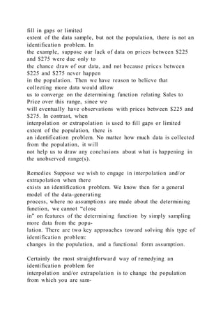
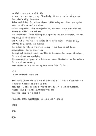
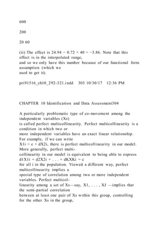
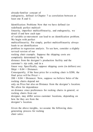
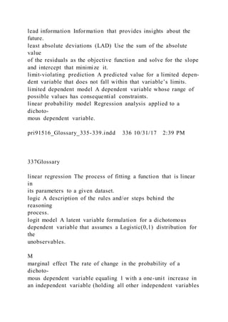
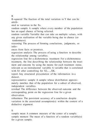
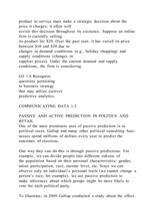
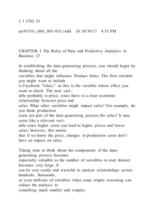
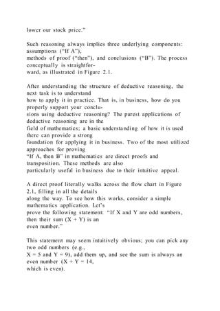
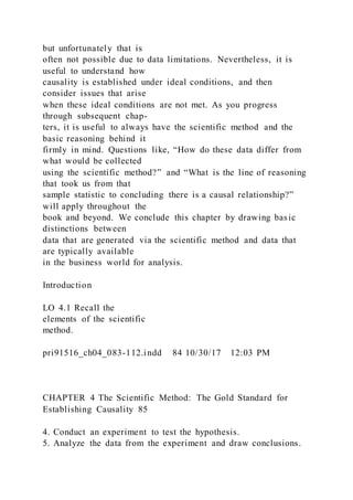
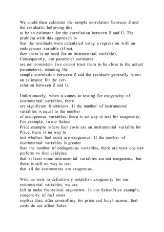
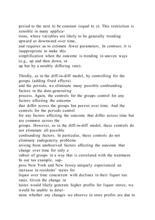
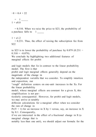
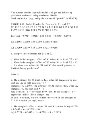
Consider again our pricing example. Here, price assignment is](https://image.slidesharecdn.com/chapter7-220921134402-19885515/85/Chapter-7-Basic-Methods-for-Establishing-Causal-Inference-Text-349-320.jpg)


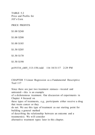


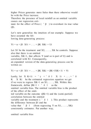
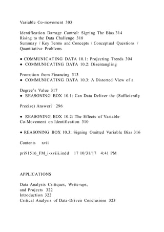
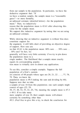
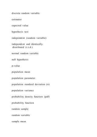
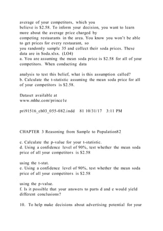
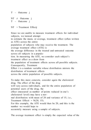
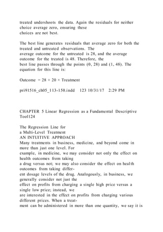
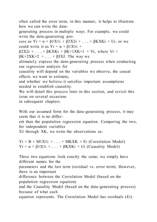
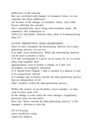
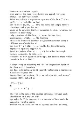
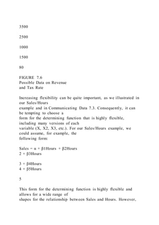
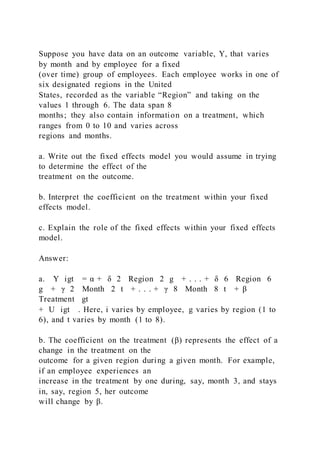
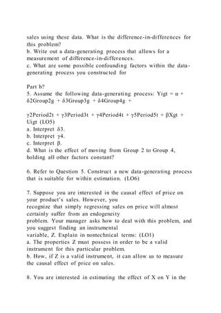
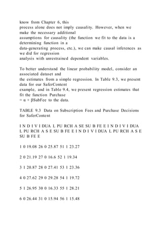
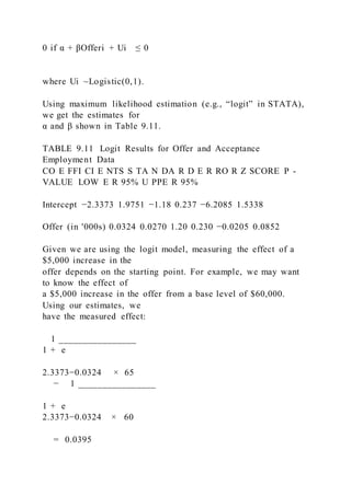
![180
170
160
150
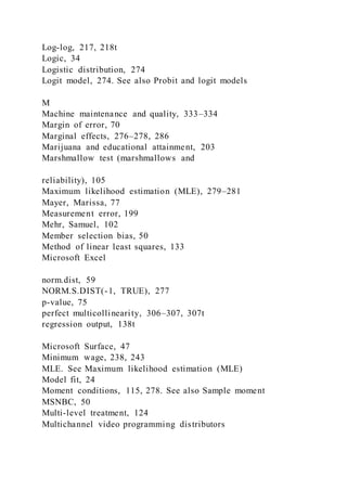
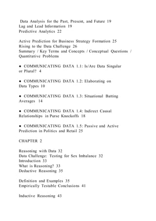
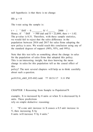
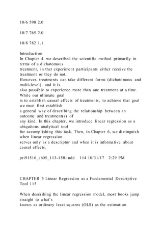
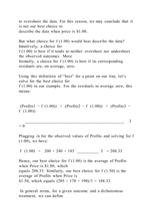
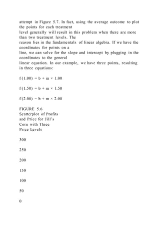
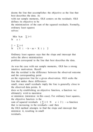
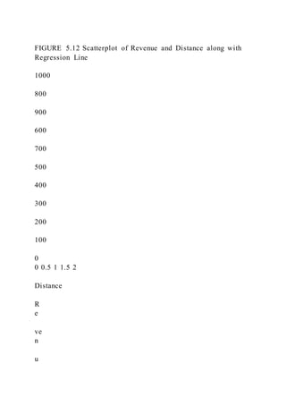
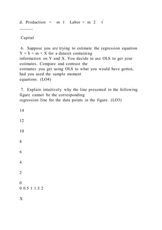
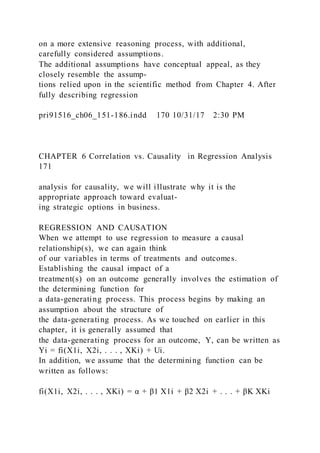
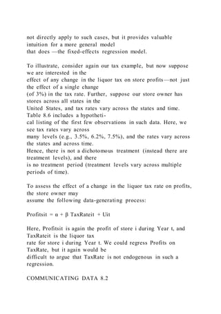
0.8 0.85 0.9 0.95 1 1.05 1.1 1.15
Price
P
ro
fi
ts
1.2
f (1.00) = 220
e1 = 20
e2 = –20
e3 = –35
pri91516_ch05_113-150.indd 121 10/31/17 2:29 PM
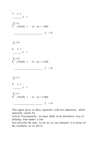
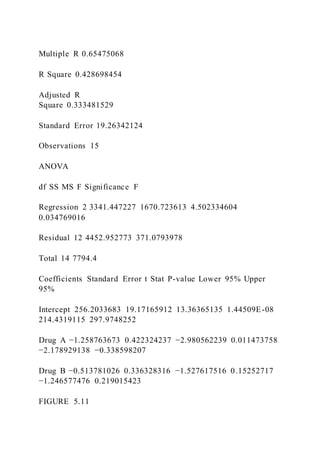
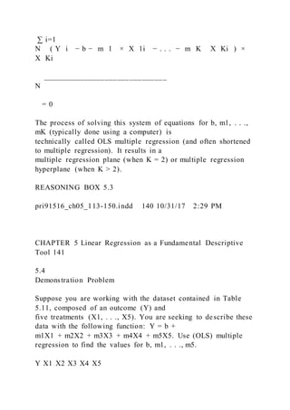
CHAPTER 5 Linear Regression as a Fundamental Descriptive
Tool122
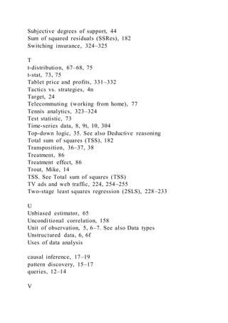
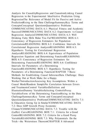
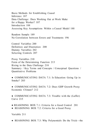
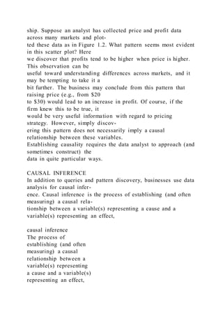
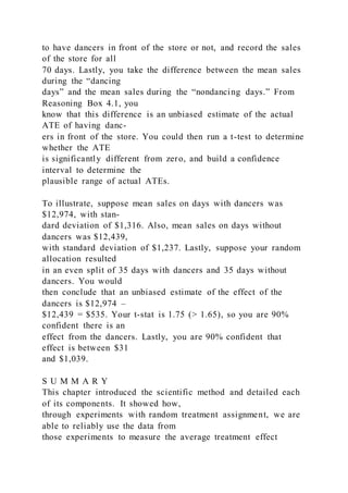
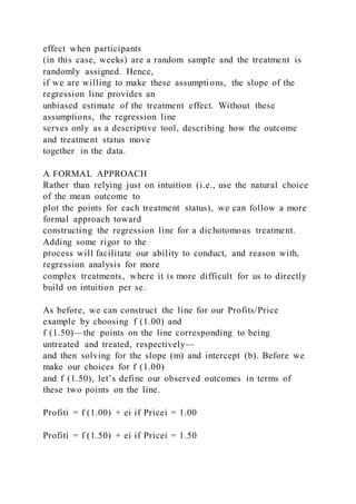
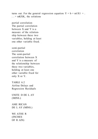
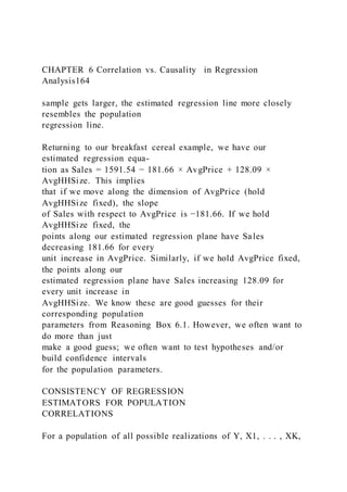
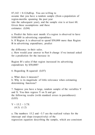
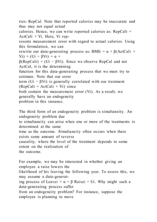
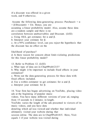
We can see from Table 5.4 that if f (1.00) = 220, then the
average residual is [20 + (−20) +
(−35)]/3 = −11.67. This implies that, on average, the point
we’ve chosen for the line tends](https://image.slidesharecdn.com/chapter7-220921134402-19885515/85/Chapter-7-Basic-Methods-for-Establishing-Causal-Inference-Text-385-320.jpg)


![pri91516_ch06_151-186.indd 152 10/31/17 2:30 PM
CHAPTER 6 Correlation vs. Causality in Regression Analysis
153
the average change in sales for those who used the program and
the average change in
sales for those who did not use the program is 15%. As a
potential client of OnlineEd, we
are likely to be interested in whether there is a causal impact of
the training program on a
firm’s subsequent sales. Here, SalesChng is the outcome,
TrainProg is the treatment, and
we would like to measure the average treatment effect (ATE) of
TrainProg on SalesChng,
where A TE = E [ SalesChng i T − SalesChng i NT ] , as
we discussed in Chapter 4. That is, we
would like to know, for a given firm, what is the expected
difference in its sales growth
between receiving the treatment (sales training) and not
receiving the treatment. We know
from Chapter 4 that assuming a random sample of firms from
the population and random
treatment assignment allows us to use the statistic given to us,
‾ SalesChng | TrainProg = 1 −
‾ SalesChng | TrainProg = 0 , as an unbiased estimate of the
ATE.
Thus far, our discussion of causality (from Chapter 4) has been
entirely in the context
of a single, dichotomous treatment, for which we measure the
ATE. However, as we dis-
cussed in Chapter 5, treatments can take on many levels and](https://image.slidesharecdn.com/chapter7-220921134402-19885515/85/Chapter-7-Basic-Methods-for-Establishing-Causal-Inference-Text-470-320.jpg)
![role of X. So, we have the
following data-generating process for the change in sales:
SalesChngi = fi(TrainProgi) + Ui
This formulation indicates that a firm i’s change in sales for a
given year is equal to a func-
tion of whether it used the sales training program, plus the
combined effect of all other
factors influencing its change in sales. The causal effect of the
training program for a given
firm is the difference in its sales growth when TrainProg
changes from 0 to 1. Using our
framework for the data-generating process, the causal effect of
the training program is:
fi(1) + Ui − (fi(0) + Ui) = fi(1) − fi(0)
Hence, when working with the data-generating process, the
causal effect for a given vari-
able on the outcome boils down to its impact on the determining
function.
There are two noteworthy features of our data-generating
process as a framework for
modeling causality. First, note that the reasoning we established
to measure an average
treatment effect using sample means easily maps into this
framework. For the OnlineEd
example, consider the following:
1. ATE = E [ SalesChng i T − SalesChng i NT ] = E [ f i
(1) + U i − ( f i (0) + U i ) ] =
E [ f i (1) − f i (0) ] . Hence, the average treatment effect
is just the expected change in
the determining function (across all individuals) when changing](https://image.slidesharecdn.com/chapter7-220921134402-19885515/85/Chapter-7-Basic-Methods-for-Establishing-Causal-Inference-Text-473-320.jpg)
![the treatment status.
2. If we assume a random sample, we know ‾ SalesChng |
TrainProg = 1 is an
unbiased estimator for E[SalesChng|TrainProg=1], which equals
E[ fi(1)] +
E[Ui|TrainProg=1] after some simple substitution and algebra.
3. If we assume a random sample, we also know ‾ SalesChng
| TrainProg = 0 is an
unbiased estimator for E[SalesChng|TrainProg=0], which equals
E[ fi(0)] +
E[Ui|TrainProg=0] again after some simple substitution and
algebra.
4. Combining 2 and 3 above, we have that ‾ SalesChng |
TrainProg = 1 −
‾ SalesChng | TrainProg = 0 is an unbiased estimator of E[
fi(1)] +
E[Ui|TrainProg=1] − E[ fi(0)] − E[Ui|TrainProg=0].
5. If we assume random treatment assignment, then conditioning
on whether the
training program was used has no impact. Consequently,
E[Ui|TrainProg=1] =
E[Ui] and E[Ui|TrainProg=0] = E[Ui]. Combining this fact with
some simple
substitution and algebra, we have E[ fi(1)] + E[Ui|TrainProg=1]
− E[ fi(0)] −
E[Ui|TrainProg=0] = E[ fi(1) − fi(0)].
6. Combining points 1–5, assuming a random sample and
random treatment
assignment implies that ‾ SalesChng | TrainProg = 1 − ‾
SalesChng | TrainProg = 0
is an unbiased estimator of the expected difference in the](https://image.slidesharecdn.com/chapter7-220921134402-19885515/85/Chapter-7-Basic-Methods-for-Establishing-Causal-Inference-Text-474-320.jpg)
![determining function
(E[ fi(1) − fi(0)]), which is the average treatment effect (ATE).
The second noteworthy feature of our data-generating process as
a framework for causal
analysis is that this framework easily extends into modeling
causality for multi-level treat-
ments and multiple treatments. If, for example, TrainProg
instead measured the number of
sales training courses taken, and so took on values of 0, 1, 2,
etc., we no longer can utilize
pri91516_ch06_151-186.indd 154 10/31/17 2:30 PM
CHAPTER 6 Correlation vs. Causality in Regression Analysis
155
the idea of the average treatment effect to measure the causal
effect of the program. In
this scenario, we have a multi-level treatment, and must then
consider the causal impacts
of different dosage levels (number of courses taken), not just
the effect of a single dose
(whether a course was taken).
However, we can easily model the causal effect of a multi -level
treatment with a
determining function in a data-generating process. Here, the
model looks just as before:
SalesChngi = fi(TrainProgi) + Ui. The causal effect of the
training program is completely
captured by fi(.); if we know this function, we can assess the
causal impact on SalesChng
for any change in TrainProg. For example, if the number of](https://image.slidesharecdn.com/chapter7-220921134402-19885515/85/Chapter-7-Basic-Methods-for-Establishing-Causal-Inference-Text-475-320.jpg)

![XK that affect Y have mean zero and are uncorrelated with X1
through XK. Then, if we
believe these assumptions, the regression equation that has the
same form as our deter-
mining function, and that best describes the population, is
equivalent to that determining
function. Reasoning Box 6.4 is highly intuitive. The population
regression equation that
best fits the data is defined by the fact that its residuals have
mean zero and are uncor-
related with the Xs. When assumption #2 holds, this means that
this feature mirrors that
of the data-generating process—the equation that best describes
the data concerning how
variables move together (correlations) also best describes the
data-generating process
(causation).
It is now practical to combine Reasoning Box 6.1 and
Reasoning Box 6.4 in order to
summarize how we can use a sample to estimate a data-
generating process. We do this in
Reasoning Box 6.5.
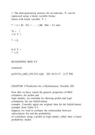
EQUIVALENCE OF POPULATION
REGRESSION EQUATION AND
DETERMINING FUNCTION
IF:
1. The data-generating process for an outcome, Y, can be
expressed as:
Yi = α + β1X1i + . . . + βKXKi + Ui
2. E [U ] = E [U × X1] = . . . = E [U × XK ] = 0](https://image.slidesharecdn.com/chapter7-220921134402-19885515/85/Chapter-7-Basic-Methods-for-Establishing-Causal-Inference-Text-530-320.jpg)
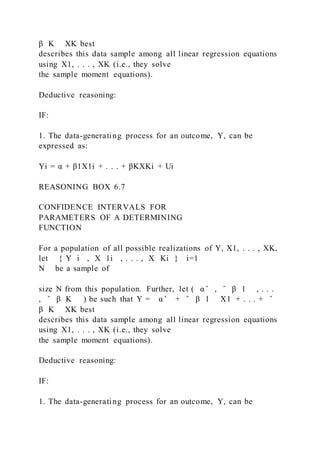
![IF:
1. The data-generating process for an outcome, Y, can be
expressed as:
Yi = α + β1 X1i + . . . + βKXKi + Ui
2. { Y i , X 1i , . . . , X Ki } i=1
N is a random sample
3. E [U ] = E [U × X1] = . . . = E [U × XK] = 0
THEN
( α ̂ , ̂ β 1 , . . . , ̂ β K ) are consistent estimators
of their corresponding parameters for the determining
function, (α, β1, . . . , βK). We write this result as:
α ̂ →α
̂ β 1 →β1
. . .
̂ β K →βK
REASONING BOX 6.5
Note that we have made one notational change within Reasoning
Box 6.5, in that we
now label the estimators from our sample as ( α ̂ , ̂ β 1 ,
. . . , ̂ β K ) rather than (b, m1, . . . , mK).
This is to highlight that, when conducting analyses of causality,
they are estimating the
parameters of a determining function, and not just the
parameters of the population regres-
sion equation. Consequently, we will use this notation for these](https://image.slidesharecdn.com/chapter7-220921134402-19885515/85/Chapter-7-Basic-Methods-for-Establishing-Causal-Inference-Text-532-320.jpg)
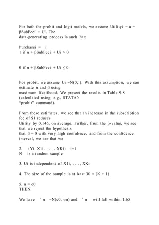
![expressed as:
Yi = α + β1X1i + . . . + βKXKi + Ui
2. { Y i , X 1i , . . . , X Ki } i=1
N is a random sample
3. E [U ] = E [U × X1] = . . . = E [U × XK ] = 0
4. The size of the sample is at least 30 × (K + 1)
5. Var(Y |X) = σ2
THEN:
The interval consisting of α ̂ plus or minus 1.65 (1.96, 2.58)
times S α ̂ will contain α approximately 90%
(95%, 99%) of the time. The same holds true for ̂ β 1 , . . .
, ̂ β K .
Inductive reasoning: Based on the observation of α ̂ , S α ̂
, and N, α is contained in the interval
( α ̂ ± 1.65 ( S α ̂ ) ) . The objective degree of support for
this inductive argument is 90%. If we instead
use the intervals ( α ̂ ± 1.96( S α ̂ ) ) and ( α ̂ ± 2.58( S
α ̂ ) ), the objective degree of support becomes 95%
and 99%, respectively.
The same holds true for ̂ β 1 , . . . , ̂ β K
REASONING BOX 6.6
pri91516_ch06_151-186.indd 176 10/31/17 2:30 PM](https://image.slidesharecdn.com/chapter7-220921134402-19885515/85/Chapter-7-Basic-Methods-for-Establishing-Causal-Inference-Text-535-320.jpg)
![CHAPTER 6 Correlation vs. Causality in Regression Analysis
177
We illustrate how to practically apply this reasoning pertaining
to causal relationships in
Demonstration Problem 6.4.
2. { Y i , X 1i , . . . , X Ki } i=1
N is a random sample
3. E [U ] = E [U × X1] = . . . = E [U × XK] = 0
4. The size of the sample is at least 30 × (K + 1)
5. Var(Y | X ) = σ2
6. α = c0
THEN:
We have α ̂ ~N ( c 0 , σ α ) and α ̂ will fall within
1.65 (1.96, 2.58) standard deviations of c0 approximately
90% (95%, 99%) of the time. This also means that α ̂ will
differ by more than 1.65 (1.96, 2.58) stan-
dard deviations from c0 (in absolute value) approximately 10%
(5%, 1%) of the time.
The same holds true for each of ̂ β 1 , . . . , ̂ β K
when assuming, e.g., βj = cj.
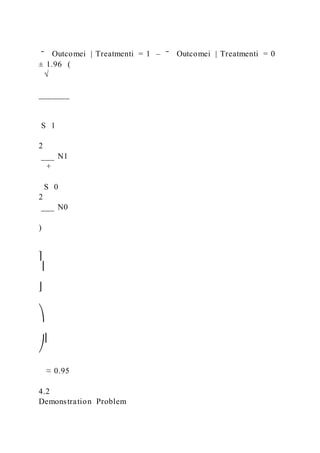
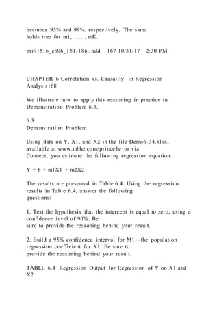
Inductive reasoning:
Using t-stats. If the absolute value of the t-stat for α ̂ ( = |
α − c0 ____ S α ̂ | ) is greater than 1.65 (1.96, 2.58), reject
the deduced (above) distribution for α ̂ . Otherwise, fail to
reject. The objective degree of support for
this inductive argument is 90% (95%, 99%).](https://image.slidesharecdn.com/chapter7-220921134402-19885515/85/Chapter-7-Basic-Methods-for-Establishing-Causal-Inference-Text-536-320.jpg)
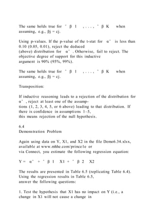
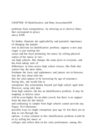
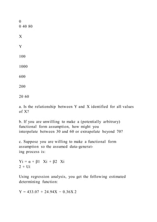
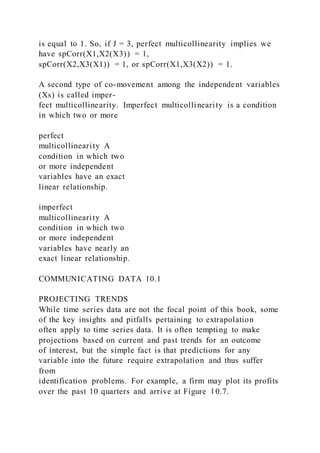
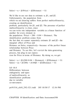
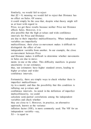
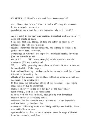
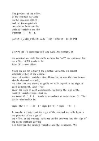
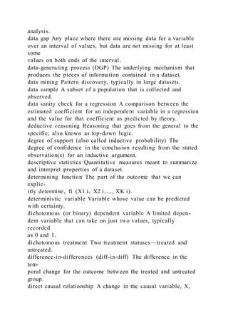
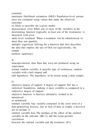
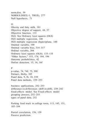
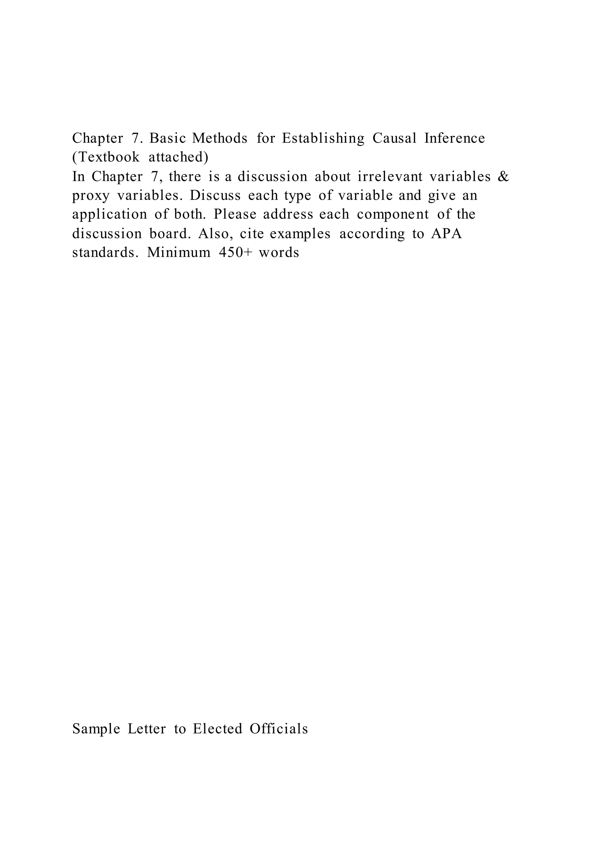
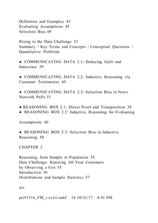
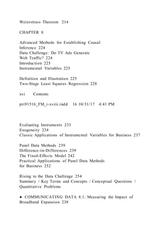
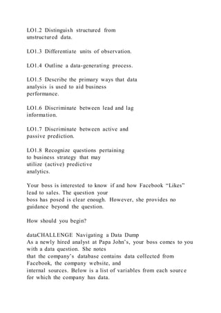
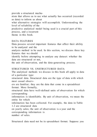
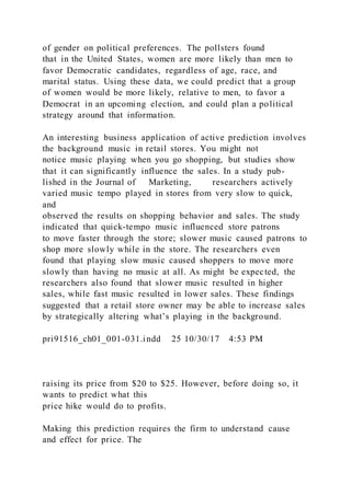
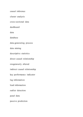
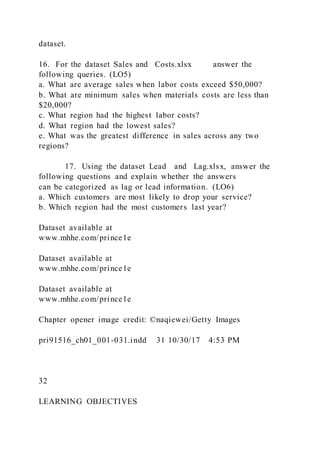
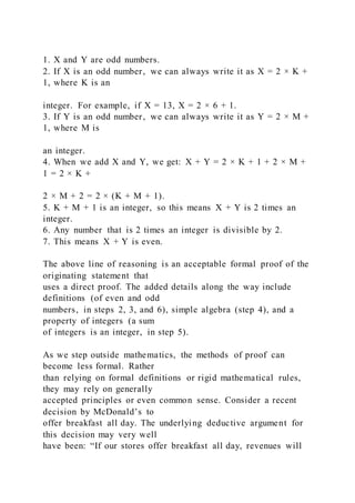
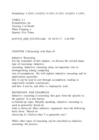
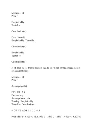
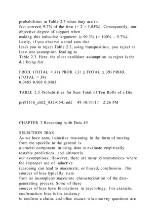
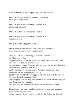
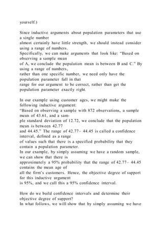
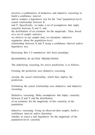
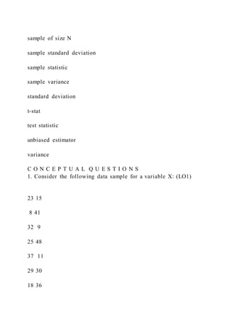
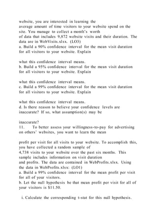
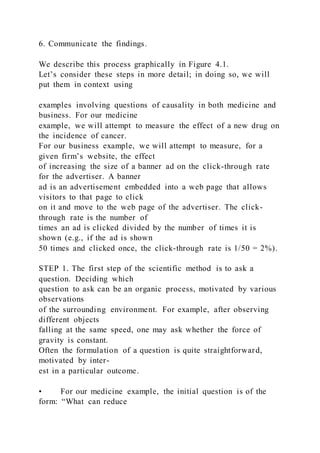
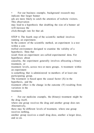
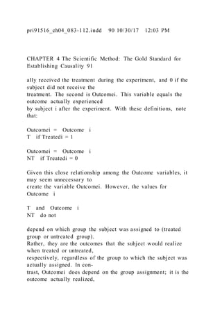
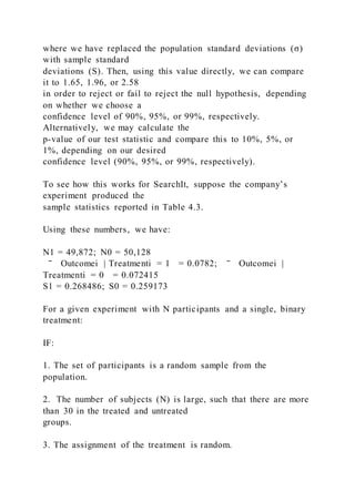
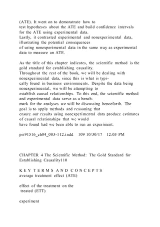
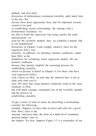
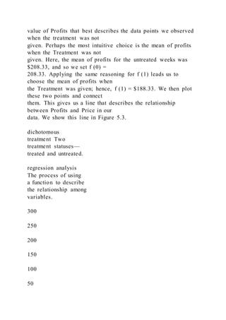
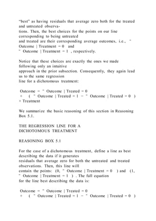
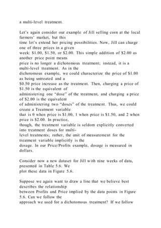
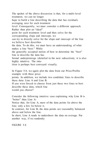
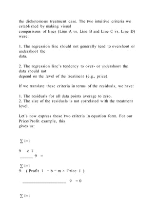
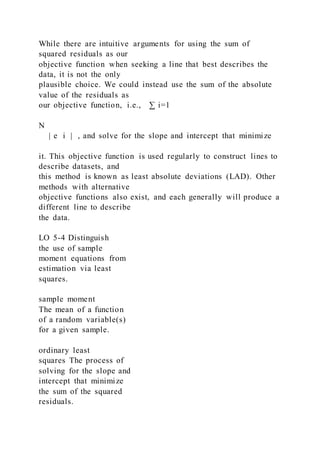
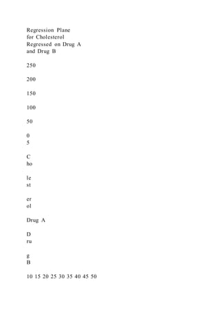
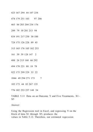
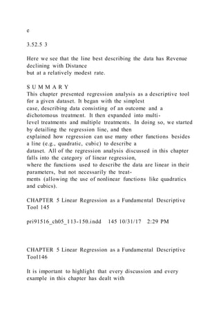
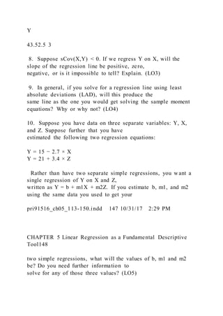
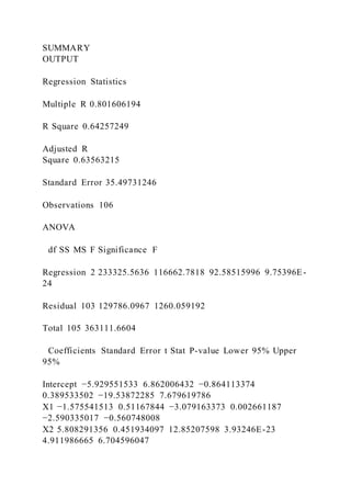
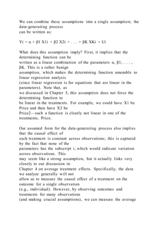
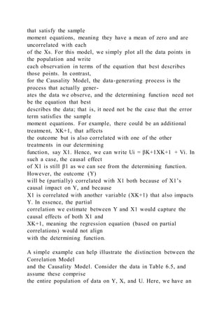
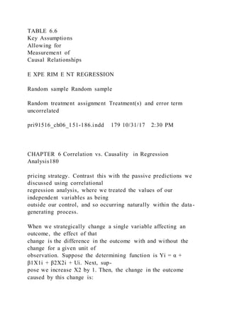
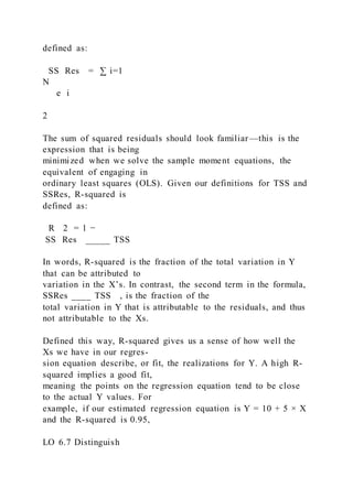
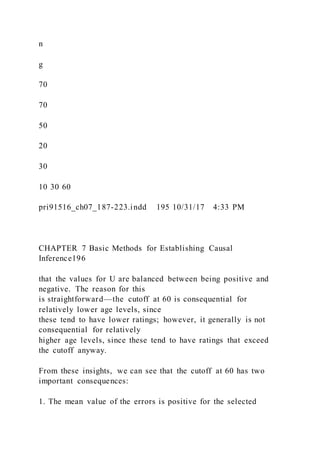
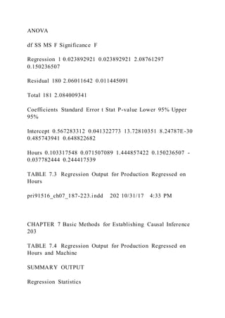
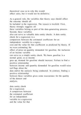
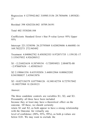
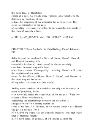
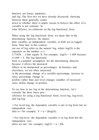
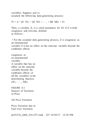
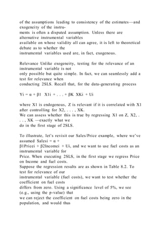
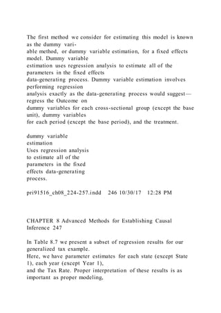
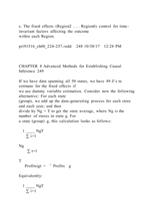
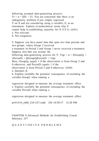
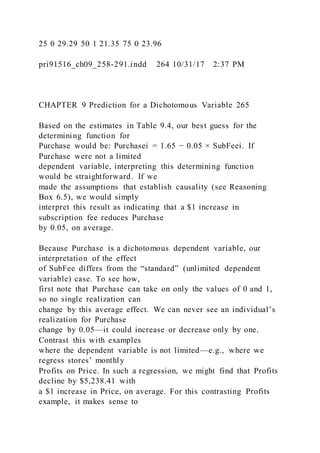
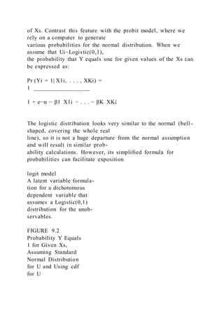
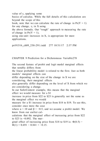
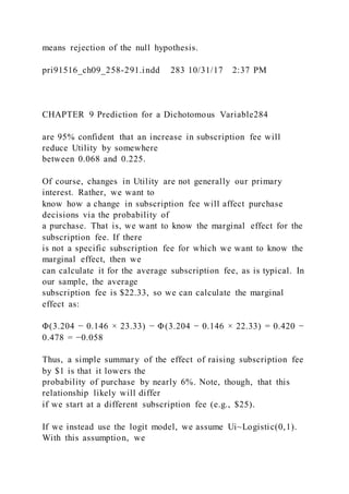
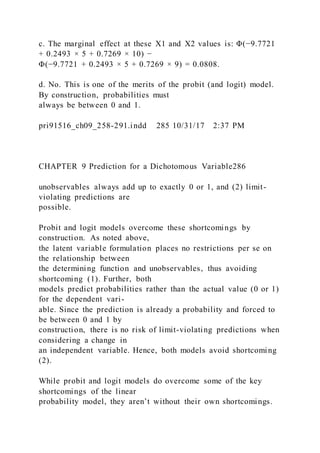
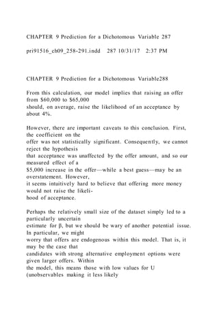
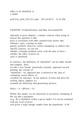
![ANOVA
df SS MS F Significance F
Regression 2 233325.5636 116662.7818 92.58515996 9.75396E-
24
Residual 103 129786.0967 1260.059192
Total 105 363111.6604
Coefficients Standard Error t Stat P-value Lower 95% Upper
95%
Intercept −5.929551533 6.862006432 −0.864113374
0.389533502 −19.53872285 7.679619786
X1 −1.575541513 0.51167844 −3.079163373 0.002661187
−2.590335017 −0.560748008
X2 5.808291356 0.451934097 12.85207598 3.93246E-23
4.911986665 6.704596047
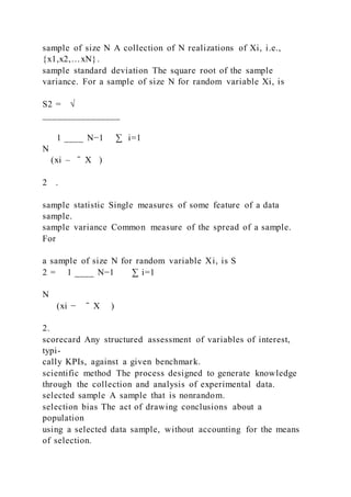
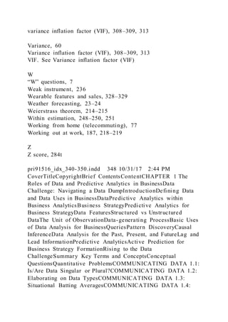
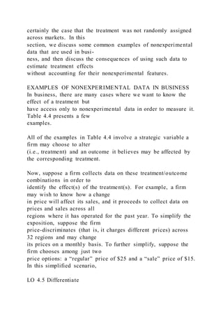
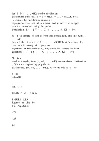
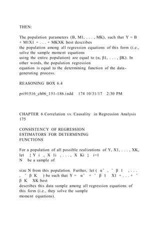
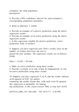
TABLE 6.5 Regression Output
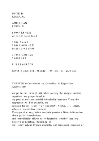
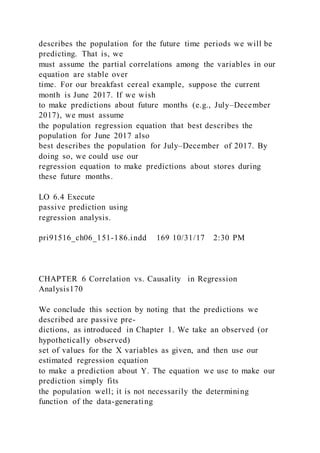
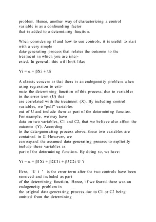
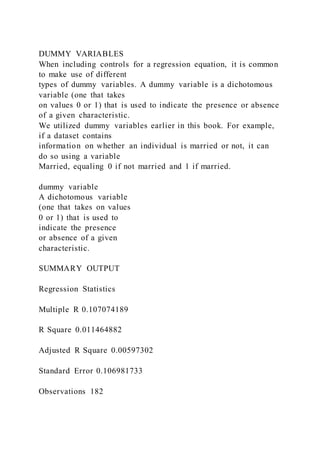
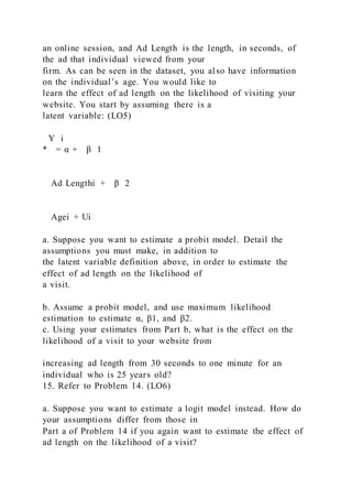
Answer:
1. We assume that: the data-generating process for Y can be
expressed as: Yi = α + β 1 X1 i +
β2X2i + Ui, we have a random sample, E [U ] = E [U × X1] = .
. . = E [U × XK ] = 0, the sample
size is at least (2 + 1) × 30 = 90, there is homoscedasticity.
Note that our fourth assumption
is immediately verified since N = 106. Note also that the first
and third assumptions are key to
ensuring our regression estimates pertain to causality rather](https://image.slidesharecdn.com/chapter7-220921134402-19885515/85/Chapter-7-Basic-Methods-for-Establishing-Causal-Inference-Text-539-320.jpg)
![than correlation only. Given these
assumptions, using a 99% confidence level, we reject the
hypothesis that X1 has no impact on Y,
since the p-value is below 0.01 (it is 0.00266).
2. We assume that: the data-generating process for Y can be
expressed as: Yi = α + β 1X 1 i +
β2X2i + Ui, we have a random sample, E [U ] = E [U × X1] = .
. . = E [U × XK] = 0, the sample
size is at least (2 + 1) × 30 = 90, there is homoscedasticity.
Note that our fourth assumption
is immediately verified since N = 106. Note also that the first
and third assumptions are key to
ensuring our regression estimates pertain to causality rather
than correlation only. Given these
assumptions, we are 95% confident that β2 is between 4.91 and
6.70.
pri91516_ch06_151-186.indd 178 10/31/17 2:30 PM
CHAPTER 6 Correlation vs. Causality in Regression Analysis
179
LINKING CAUSAL REGRESSION TO THE EXPERIMENTAL
IDEAL
Now that we have established the assumptions that allow us to
estimate the parameters of a
determining function, we can draw parallels between regression
analysis establishing cau-
sality and the experimental ideal. In Chapter 4, we showed that
having a random sample
and random treatment assignment allowed us to use differences
in mean outcomes between
the treated and untreated to measure the average treatment](https://image.slidesharecdn.com/chapter7-220921134402-19885515/85/Chapter-7-Basic-Methods-for-Establishing-Causal-Inference-Text-540-320.jpg)
![and vice versa.
A simplified version of this experiment would involve
developing a rating system indicating whether a news feed was
positive or not (e.g., PosFeed = 1 if news feed is positive and 0
if negative), and indicating whether an individual’s status
was positive or not (e.g., PosStat = 1 if status is positive and 0
if negative). For the experiment, we can randomly assign
news feeds with different positivity ratings across individuals
(treatment) and observe the positivity rating of the individuals’
statuses (outcome). Then, we know that if we assume the
individuals in the study are a random sample and treatment was
randomly assigned, the difference in the positivity in status
across the two groups is a reliable measure of the causal effect
of news feed positivity.
Consider the same analysis within a regression framework for
estimating causality. Here, we assume the data-generat-
ing process is PosStati = α + β PosFeedi + Ui. We’ve already
assumed we have a random sample, and random treatment
assignment ensures no correlation between unobserved factors
affecting status (U ) and the news feed (PosFeed). If we
further assume that E [U] = 0 (easily satisfied when there is a
constant term, i.e., α, in the data-generating process), then
from Reasoning Box 6.5, we know α ̂ and β ̂ —the
intercept and slope that best describe the sample data—are
consistent
estimators for the parameters of the determining function.
Hence, we see again how running an experiment with random
treatment assignment allows us to measure causal relationships.
pri91516_ch06_151-186.indd 180 10/31/17 2:30 PM
CHAPTER 6 Correlation vs. Causality in Regression Analysis](https://image.slidesharecdn.com/chapter7-220921134402-19885515/85/Chapter-7-Basic-Methods-for-Establishing-Causal-Inference-Text-545-320.jpg)
![181
with a change in a treatment—something we did not directly
observe for any element of
the population, even those in the sample.
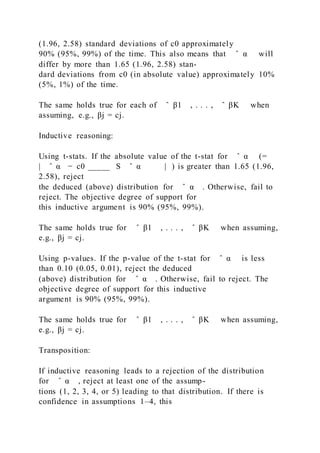
For our prediction that sales will increase by 181.66 when
average price declines by one
dollar to be accurate, we must believe that our estimated
regression equation is a consis-
tent estimate of the determining function. A key assumption for
this to be true is that our
independent variables are uncorrelated with the error term. This
means that average price
must be uncorrelated with other factors that influence sales.
In the previous section, we conjectured that average age of a
store’s customers may impact
sales and the average price for that store. When conducting
passive prediction, this rela-
tionship among average age, average price, and sales is not
consequential—our estimated
regression equation still provides a consistent estimate of
partial correlations, which is all
we are seeking for passive prediction. However, when
conducting active prediction, this
relationship is highly consequential. It implies that, within our
assumed data-generating
process (Sales = α + β1AvgPrice + β2AvgHHSize + U), we have
E[AvgPrice × U] ≠ 0.
As a result, ̂ β 1 is not a consistent estimator for β1,
meaning an increase of 181.66 is not a
consistent prediction for the change in sales when price
exogenously declines by one dollar.
This is because ̂ β 1 captures a combination of the causal
effect of price and the causal effect](https://image.slidesharecdn.com/chapter7-220921134402-19885515/85/Chapter-7-Basic-Methods-for-Establishing-Causal-Inference-Text-546-320.jpg)
![sum of squared residuals
total sum of squares
unconditional correlation
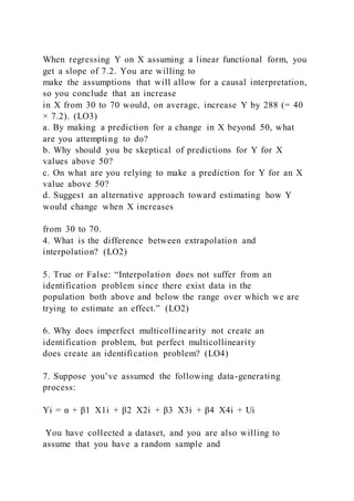
C O N C E P T U A L Q U E S T I O N S
1. The unconditional correlation between Y and X1 is 0.72, but
the semi-partial correlation between Y and
X1 controlling for X2 is 0.03. What does this imply about the
unconditional correlation between: (LO2)
a. Y and X2?
b. X1 and X2?
c. Given the above information, does the sign of the
unconditional correlation between Y and X2 have
any relationship with the sign of the unconditional correlation
between X1 and X2? (If Corr(Y, X2) > 0,
does this tell us that Corr(X1, X2) > 0?)
2. What additional assumptions are needed to conclude that the
regression estimators are consistent
estimates of the parameters of a determining function, beyond
those needed to conclude they are
consistent estimators of the parameters of a population
regression equation? (LO5)
2. { Revenue i , Distance i } i=1
N is a random sample
3. E [U] = E [U × Distance] = 0
If these assumptions hold, −56.18 is a consistent estimate of the](https://image.slidesharecdn.com/chapter7-220921134402-19885515/85/Chapter-7-Basic-Methods-for-Establishing-Causal-Inference-Text-555-320.jpg)
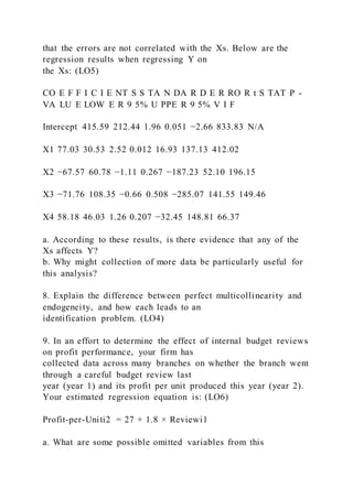
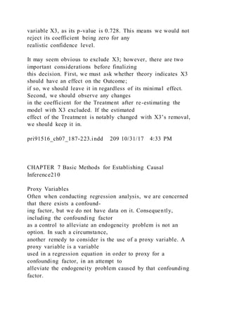
![satisfaction. In an attempt to
improve job satisfaction, you have conducted a survey of all
employees, collecting informa-
tion on: job satisfaction (0–100), years of education, sex, hours
per week at the company
gym, and pay grade (1–5). Management is considering providing
incentives for employees
to exercise more during work hours, but is unsure whether doing
so is likely to make a
difference in employee job satisfaction.
How can you use your survey to inform this decision?
pri91516_ch07_187-223.indd 187 10/31/17 4:33 PM
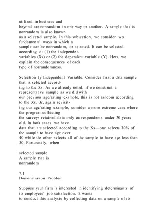
CHAPTER 7 Basic Methods for Establishing Causal
Inference188
Assessing Key Assumptions Within
a Causal Model
Recall from Reasoning Box 6.5 the assumptions that imply our
regression estimators con-
sistently estimate the parameters of a determining function.
These assumptions are:
1. The data-generating process for an outcome, Y, can be
expressed as:
Yi = α + β1X1i + . . . + βKXKi + Ui
2. {Yi, X1i, . . . , XKi} i=1
N is a random sample.
3. E[U] = E[U × X1] = . . . = E[U × XK] = 0](https://image.slidesharecdn.com/chapter7-220921134402-19885515/85/Chapter-7-Basic-Methods-for-Establishing-Causal-Inference-Text-563-320.jpg)


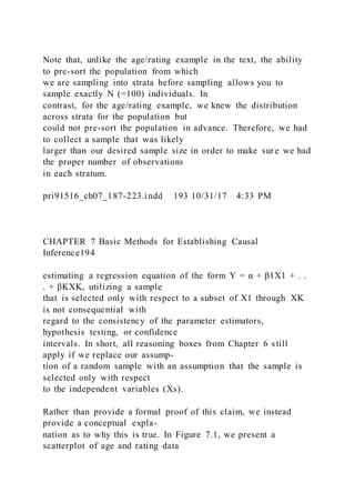
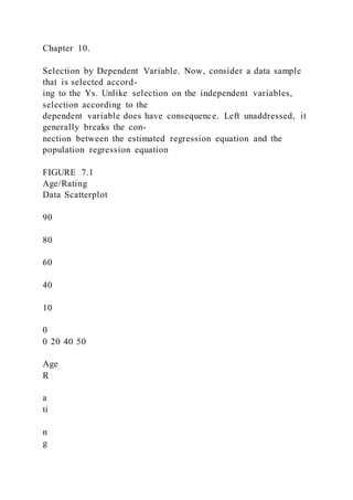
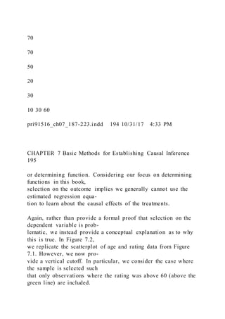
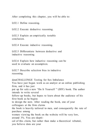
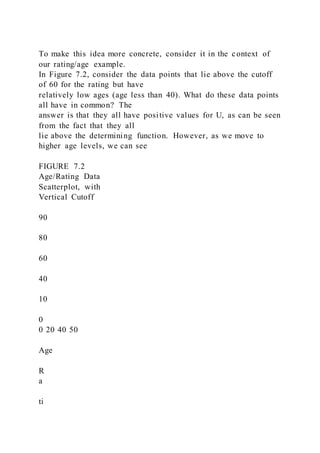
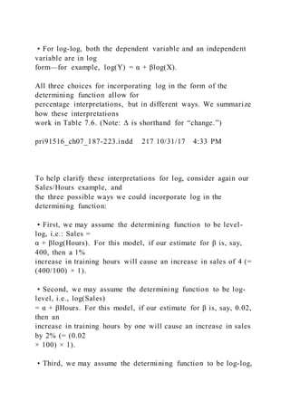
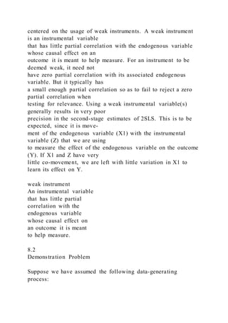
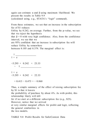
![In addition to the vertical cutoff at 60, we also include the
actual determining function
for the data-generating process that produced these data (the
black line). In fact, the data-
generating process that produced these data is: Ratingi = 40 +
0.5Agei + Ui, where each
Ui is independent (of all other Us and Age) and normal with
mean zero and variance of
25. Hence this data-generating process has E[Ui] = E[AgeiUi] =
0, and so with a random
sample, the estimated regression line is a consistent estimator of
the determining function.
We’ll now show how selection on rating (the dependent
variable) can cause a problem
when attempting to use these data to estimate a determining
function (conduct causal anal-
ysis). We’ll show how selection on the dependent variable tends
to create a situation where
E[Ui] = E[XiUi] = 0 may hold true for the full population, but
E[Ui] ≠ 0 and E[XiUi] ≠ 0
for the selected subset of the population. That is, the errors do
not have mean zero or
zero correlation with the independent variables for the selected
subset of the population.
Consequently, when we solve the moment equations by forcing
the residuals to have zero
mean and zero correlation with the independent variables for the
selected sample, these
conditions do not match what is happening for the
corresponding selected subset of the
population from which the sample was drawn. Hence, our
estimators no longer consis-
tently estimate the parameters of the determining function,
meaning they are no longer
reliable for causal analysis.](https://image.slidesharecdn.com/chapter7-220921134402-19885515/85/Chapter-7-Basic-Methods-for-Establishing-Causal-Inference-Text-583-320.jpg)
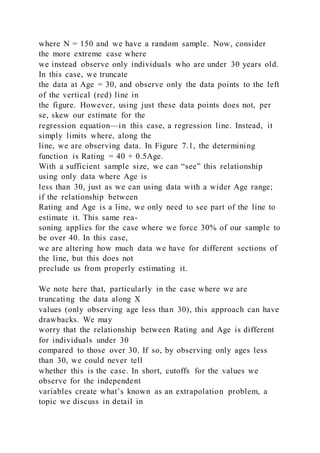
![subset.
2. The errors and age are negatively correlated.
We know consequence 1 is true since the errors have mean zero
for relatively high ages but
tend to be positive for relatively low ages. We know
consequence 2 is true since relatively
low ages tend to correspond to relatively high errors.
We conclude by noting there are corrective measures one can
take to address selection
issues, particularly the highly problematic issue of selection on
outcomes. For example,
we can make assumptions about the method of selection and
adjust our estimation
procedure(s) accordingly. Such estimation techniques are
outside the scope of this book,
but for our purposes, it is an important step to be aware of
whether a sample is selected
and whether the type of selection is consequential toward your
findings.
NO CORRELATION BETWEEN ERRORS AND
TREATMENTS
The third assumption we make to ensure our regression
estimates are good guesses for
the parameters of the determining function is that E[Ui] =
E[X1iUi] = . . . = E[XKiUi] = 0
for the data-generating process Yi = α + β1X1i + . . . + βKXKi
+ Ui. That is, we assume the
errors have mean zero and are not correlated with the treatments
in the population. As we
noted when first presenting this assumption, the part that
assumes the errors have zero mean
is generally satisfied when there is an intercept term in the
determining function. In some](https://image.slidesharecdn.com/chapter7-220921134402-19885515/85/Chapter-7-Basic-Methods-for-Establishing-Causal-Inference-Text-586-320.jpg)

![makes good sense since we
expect fewer people to buy a product as its price rises.
So, how is it that our estimates violate the law of demand,
rendering them clearly inaccu-
rate? Here, we likely have a violation of assumption 3; it is
likely the case that unobserved
factors affecting quantity demanded are correlated with Price
(i.e., E[PriceiUi] ≠ 0).
There are many possible confounding factors: one candidate
would be local income levels.
In particular, we don’t expect managers to set prices for their
products randomly. Instead,
they observe the local demand conditions and try to set a price
they believe will be most
profitable. One local demand condition on which they may base
their price decision is
local income levels. They may choose to set a higher price when
local income is high and
a lower price when local income is low. If this is the case, we
then have our violation,
since local income likely affects quantity demanded (it is part
of U), and it is correlated
with the price, meaning we have E[PriceiUi] ≠ 0. The presence
of this other factor gives
the illusion that customers like higher prices. When local
demand is “good” (local income
levels are high), people tend to buy more of the product and the
price tends to be higher,
and vice versa.
Consider an alternative version of this example where we also
have data on local income
levels (measured as average income among households in the
region); that is, we now have
the data in the fourth column of Table 7.2 as well. We can then](https://image.slidesharecdn.com/chapter7-220921134402-19885515/85/Chapter-7-Basic-Methods-for-Establishing-Causal-Inference-Text-590-320.jpg)


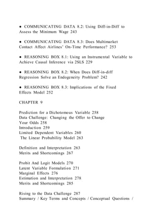
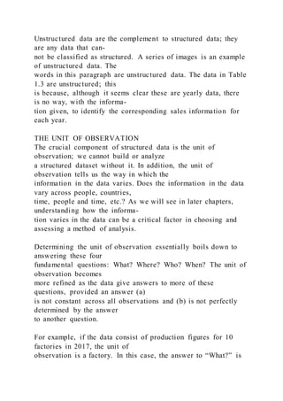
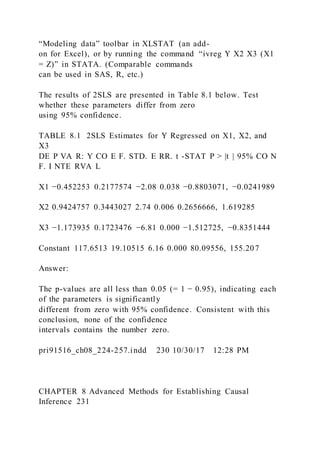
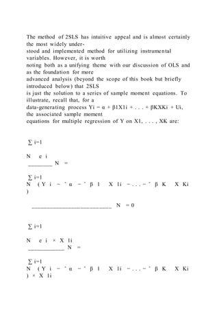
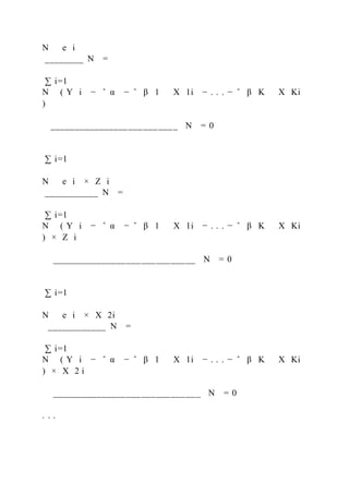
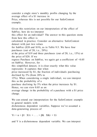
![As described above, the execution of 2SLS is quite
straightforward—simply run two
consecutive regressions, using the predictions from the first as
an independent variable
in the second. In practice, we seldom see analysts run each
regression separately, for two
reasons: (1) Virtually all statistical software combines this
process into a single com-
mand. (2) 2SLS, as described in Reasoning Box 8.1, provides
only consistent estimates; it
does not ensure our ability to run hypothesis tests and build
confidence intervals. It may
be tempting to simply use the p-values, t-stats, etc., from the
second-stage regression to
perform these tasks; however, these will tend to be inaccurately
measured unless corrective
procedures are taken.
USING AN INSTRUMENTAL VARIABLE TO
ACHIEVE CAUSAL INFERENCE VIA 2SLS
IF:
1. The data-generating process for an outcome, Y, can be
expressed as:
Yi = α + β1 X1i + . . . + βK XKi + Ui
2. { Y i , X 1i , . . . , X Ki , Z i } i=1
N is a random sample
3. E [U] = E [U × X2] = . . . = E [U × XK] = 0
4. The size of the sample is at least 30 × (K + 1)](https://image.slidesharecdn.com/chapter7-220921134402-19885515/85/Chapter-7-Basic-Methods-for-Establishing-Causal-Inference-Text-671-320.jpg)
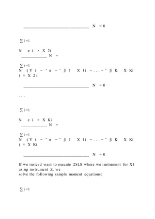


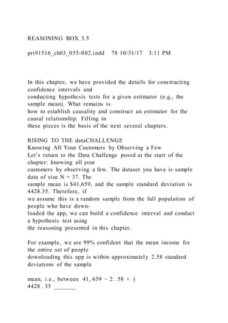
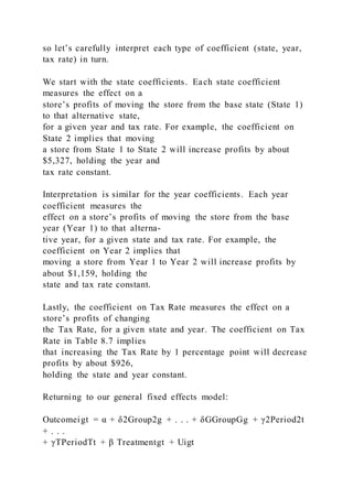
![conclude it is relevant.
It is important to note that, when testing for relevance of an
instrument in the first stage
of 2SLS, we are not testing for a causal effect of the
instrumental variable (Z) on the out-
come (Y). An instrument, Z, is still relevant even if the
relationship with the endogenous
variable, say X1, is purely correlational and not causal.
Consequently, as was noted in
Reasoning Boxes 6.2 and 6.3, we can build confidence intervals
and run hypothesis tests
concerning partial correlations by just assuming: (1) a random
sample, (2) a large sample
[30 × (K + 1)], and (3) homoscedasticity (Var(Y | X) = σ2). We
then test for relevance just
as we test for population correlations with regression.
Testing for relevance when there are multiple instrumental
variables is similar to the
case with just one. For simplicity, consider a data-generating
process
Yi = α + β1X1i + . . . + βKXKi + Ui
where X1 is endogenous and we are considering Z1 and Z2 as
instrumental variables for X1.
Again, we test for relevance using the first-stage regression,
where we’ve regressed X1 on
Z1, Z2, X2, . . . , XK. Just as with a single instrumental
variable, we can test whether either of
the coefficients on Z1 and Z2 differs from zero by, for instance,
looking at their p-values. In
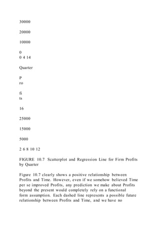
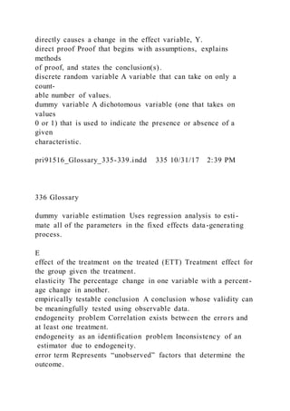
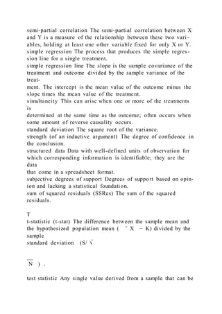
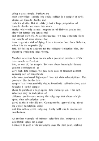
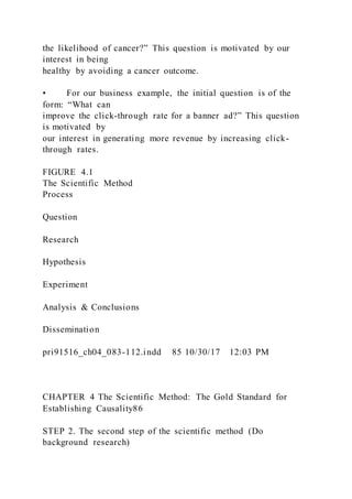
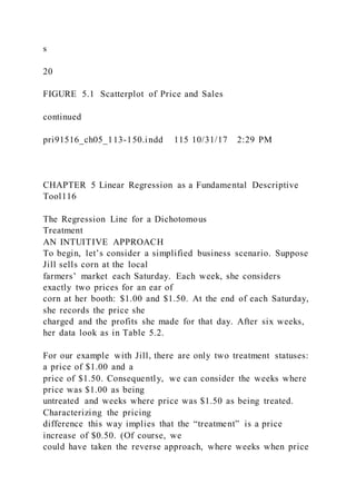
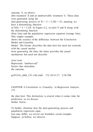
TABLE 8.2 Regression Output for Price Regressed on Income
and Fuel Costs](https://image.slidesharecdn.com/chapter7-220921134402-19885515/85/Chapter-7-Basic-Methods-for-Establishing-Causal-Inference-Text-690-320.jpg)


![) + Ui
This alternative functional form may seem helpful toward
limiting the associated values
for Purchase, since 1 _____ SubFee will be between 0 and 1
for any subscription fee more than $1.
However, there is no restriction on β (or α), so we could still
end up with limit-violating
predictions, e.g., predictions above 1 for Purchase if β is a large
number.
9.1
Demonstration Problem
An outcome variable, Y, can take on only the values 0 or 1. In
attempting to measure the effects of X1 and
X2 on Y, you’ve collected a sample of size 200 on these three
variables, and assumed the following:
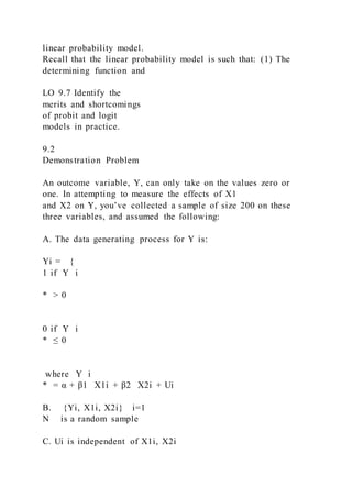
A. The data-generating process for Y is: Yi = α + β1X1i +
β2X2i + Ui
B. {Yi, X1i, X2i} i=1
200 is a random sample
C. E [U ] = E [U × X1] = E [U × X2] = 0
You regress Y on X1 and X2, which yields the results in Table
9.6.
TABLE 9.6 Regression Results for Y Regressed on X1 and X2
CO E F F I C I E NT S
S TA N DA R D
E R R O R t S TAT P -VA LU E LOW E R 9 5% U PPE R 9 5%](https://image.slidesharecdn.com/chapter7-220921134402-19885515/85/Chapter-7-Basic-Methods-for-Establishing-Causal-Inference-Text-778-320.jpg)


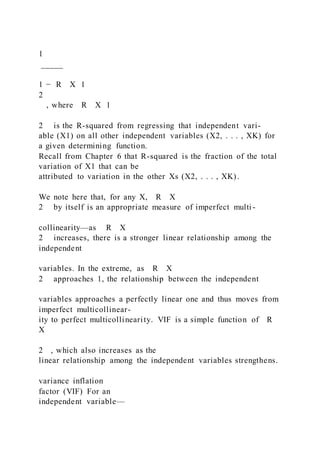
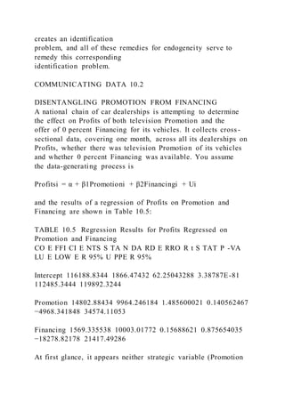
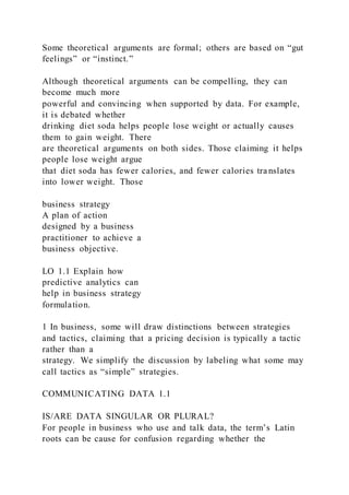
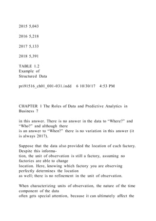
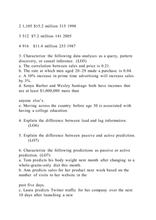
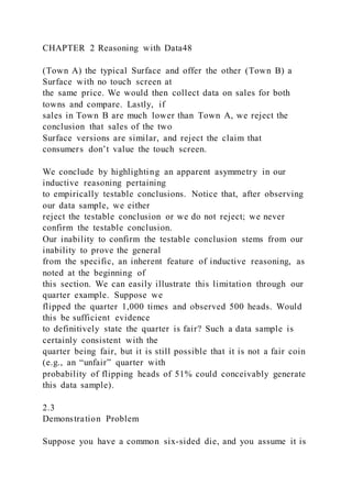
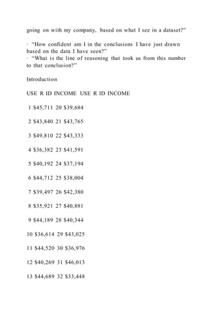
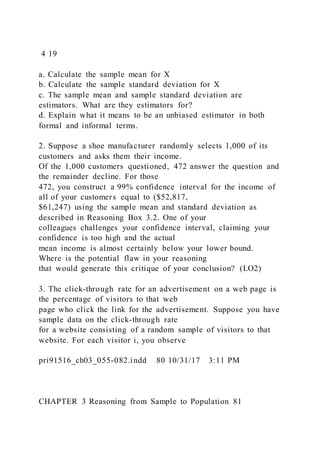
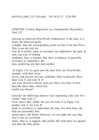
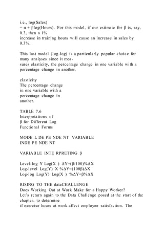
![we define X to be the number of 3s we observe on a single roll
of the die (X = 1 if we roll
a 3 and X = 0 if we roll any other number), we have E[X ] = p.
Some additional math would
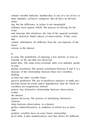
identified Can be
estimated with any
level of precision given
a large enough sample
from the population.
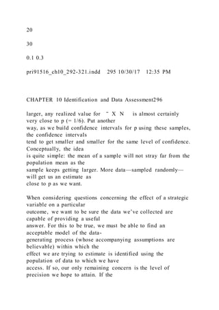
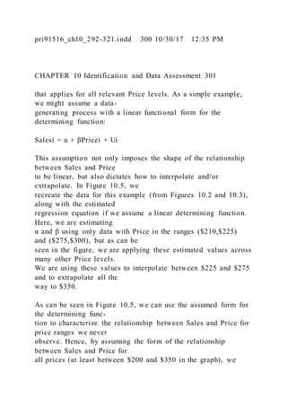
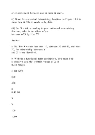
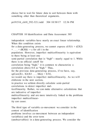
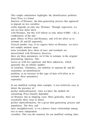
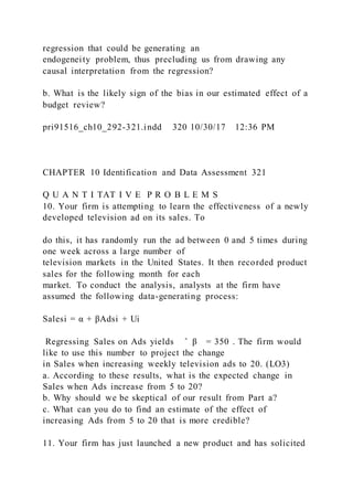
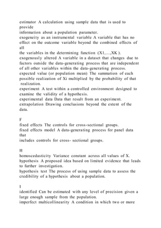
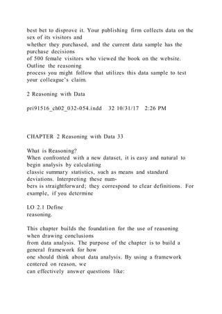
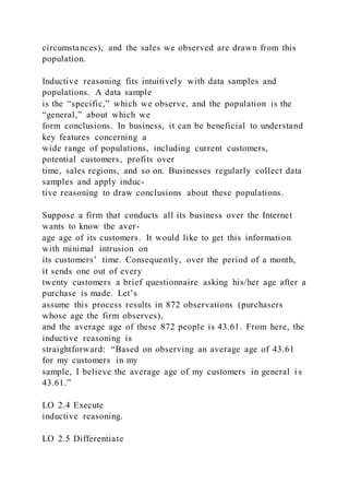
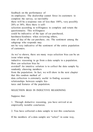
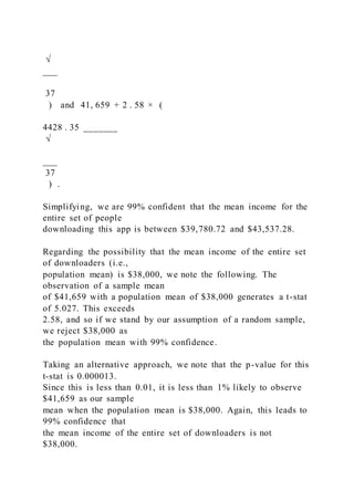
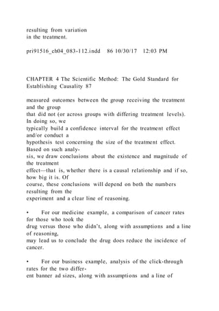
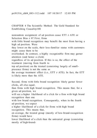
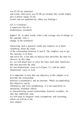
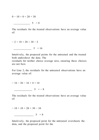
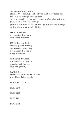
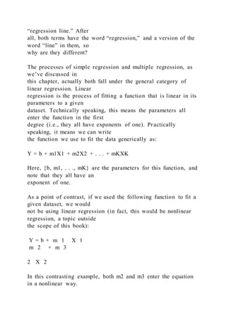
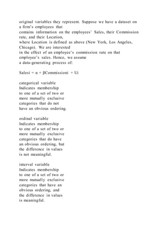
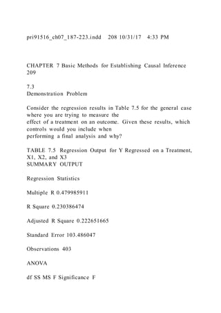
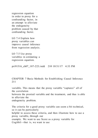
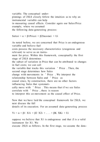
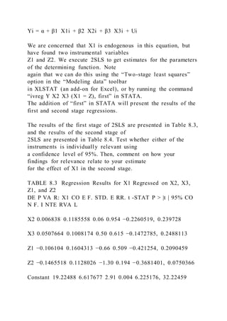
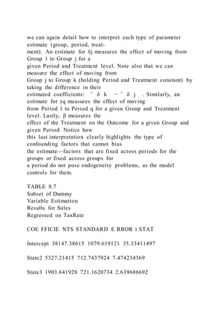
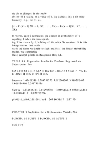
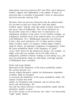
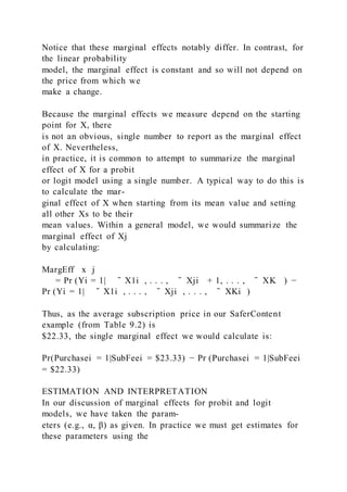
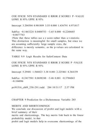
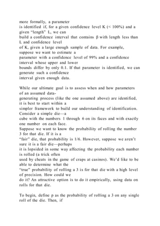
IP LOCATION ZIP CODE PRICE SALES
90006 $297.32 8
32042 283.75 9
45233 275.35 7
07018 280.25 11
53082 223.50 17
53039 214.10 12
37055 292.90 8
TABLE 10.2
Subsample of Rocking
Chair Data
pri91516_ch10_292-321.indd 294 10/30/17 12:35 PM
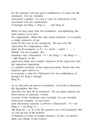
CHAPTER 10 Identification and Data Assessment 295](https://image.slidesharecdn.com/chapter7-220921134402-19885515/85/Chapter-7-Basic-Methods-for-Establishing-Causal-Inference-Text-845-320.jpg)
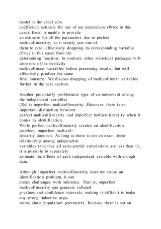
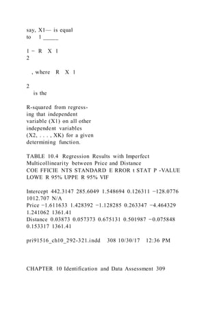
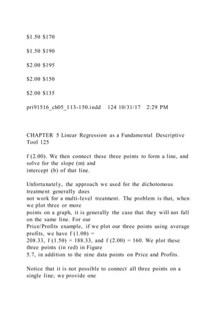
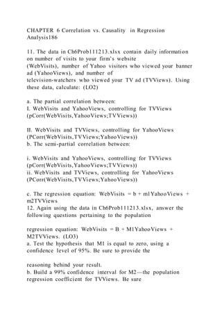
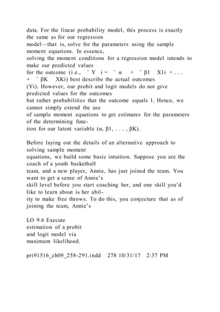
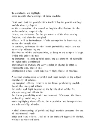
![show that Var[X ] = p(1 − p). Within this simple framework, the
parameter p is identified.
In other words, we can estimate p as precisely as we want given
enough data on the die
(given enough rolls of the die).
The fact that p is identified follows directly from the central
limit theorem (discussed in
Chapter 3). Suppose we roll the die N times. Define x1 as the
observed value of X for the first
roll, x2 for the second, and so on. Then, define ‾ X N =
1 __ N [x1 + x2 + . . . +xN] =
1
__
N
∑ i=1
N
xi, i.e., the
sample mean for X, or equivalently, the proportion of the N
rolls that showed a 3. Given these
definitions, the central limit theorem states that ‾ X N ∼ N
(p,
√
_______
p(1 − p)
_______
√
__](https://image.slidesharecdn.com/chapter7-220921134402-19885515/85/Chapter-7-Basic-Methods-for-Establishing-Causal-Inference-Text-846-320.jpg)