Downloaded 145 times


![4.3.2 The Prefix-Sum Operation
Also known as scan operation
Used for associative operations other than addition for
finding like maximum, minimum, string concatenations
and Boolean operations
Example:
Given p numbers n0,n1,…,np-1 (one on each node), the problem
is to compute the sums sk = ∑i
k
= 0 ni for all k between 0 and p-1 .
Initially, nk resides on the node labeled k, and at the end of the
procedure, the same node holds Sk.
[Wilkinson, P-172]
53](https://image.slidesharecdn.com/chapter4pc-150609040921-lva1-app6892/75/Chapter-4-pc-53-2048.jpg)


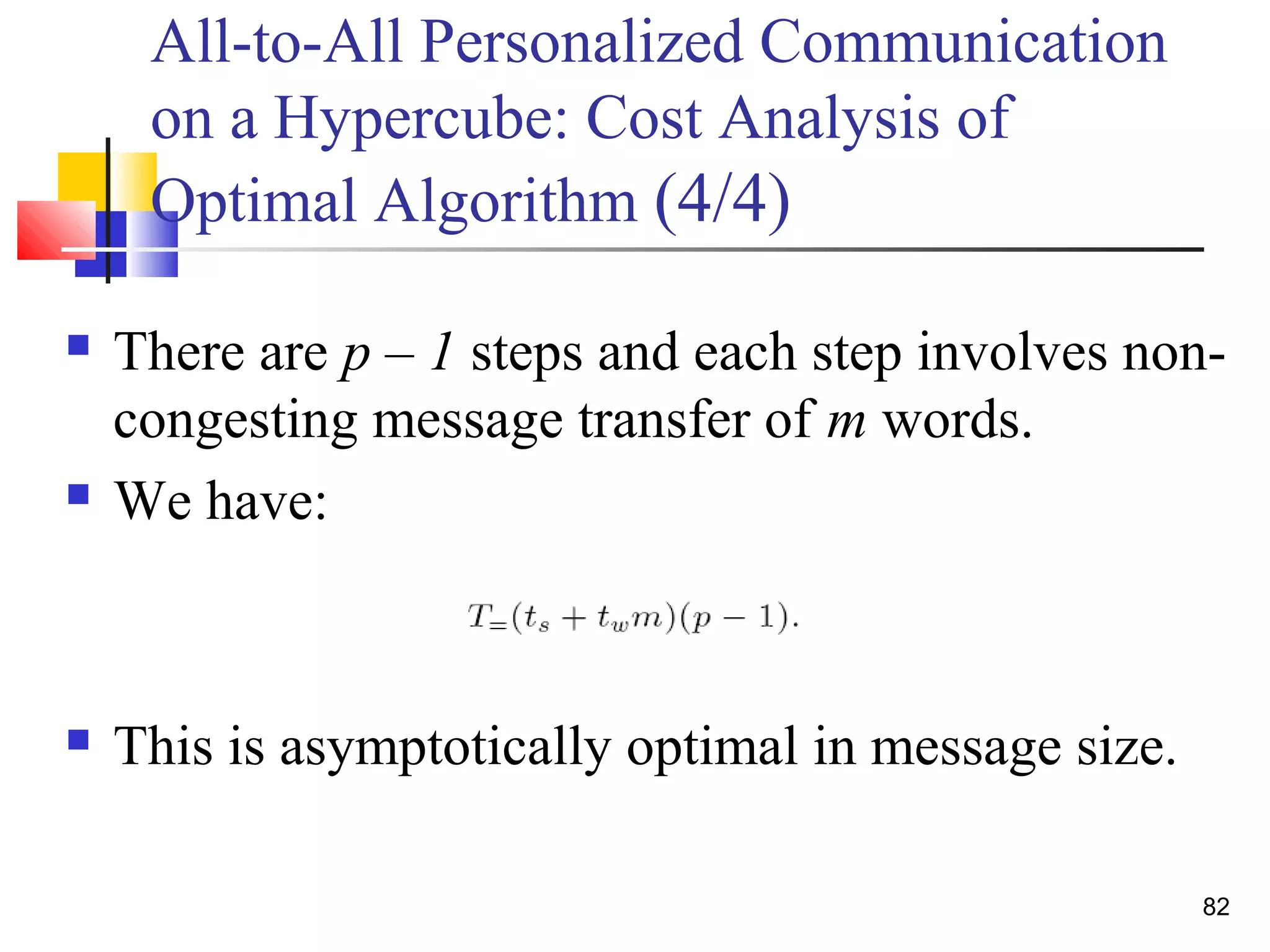
![Non-optimality in Hypercube
algorithm(4/4)
Each node send m(p-1) words of data
Average distance of communication (log p)/2
Total network traffic is pxm(p-1)x(log p)/2
Total number of links is (p log p)/2
The lower bound for communication time is
T= [twpxm(p-1)x(log p)/2]/ (p log p)/2
=twm(p-1)
78](https://image.slidesharecdn.com/chapter4pc-150609040921-lva1-app6892/75/Chapter-4-pc-78-2048.jpg)


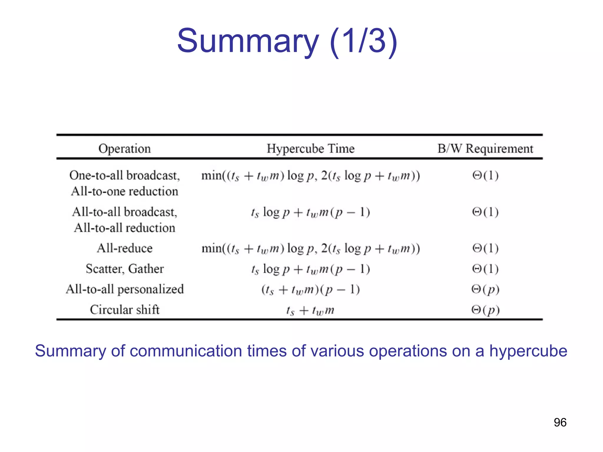


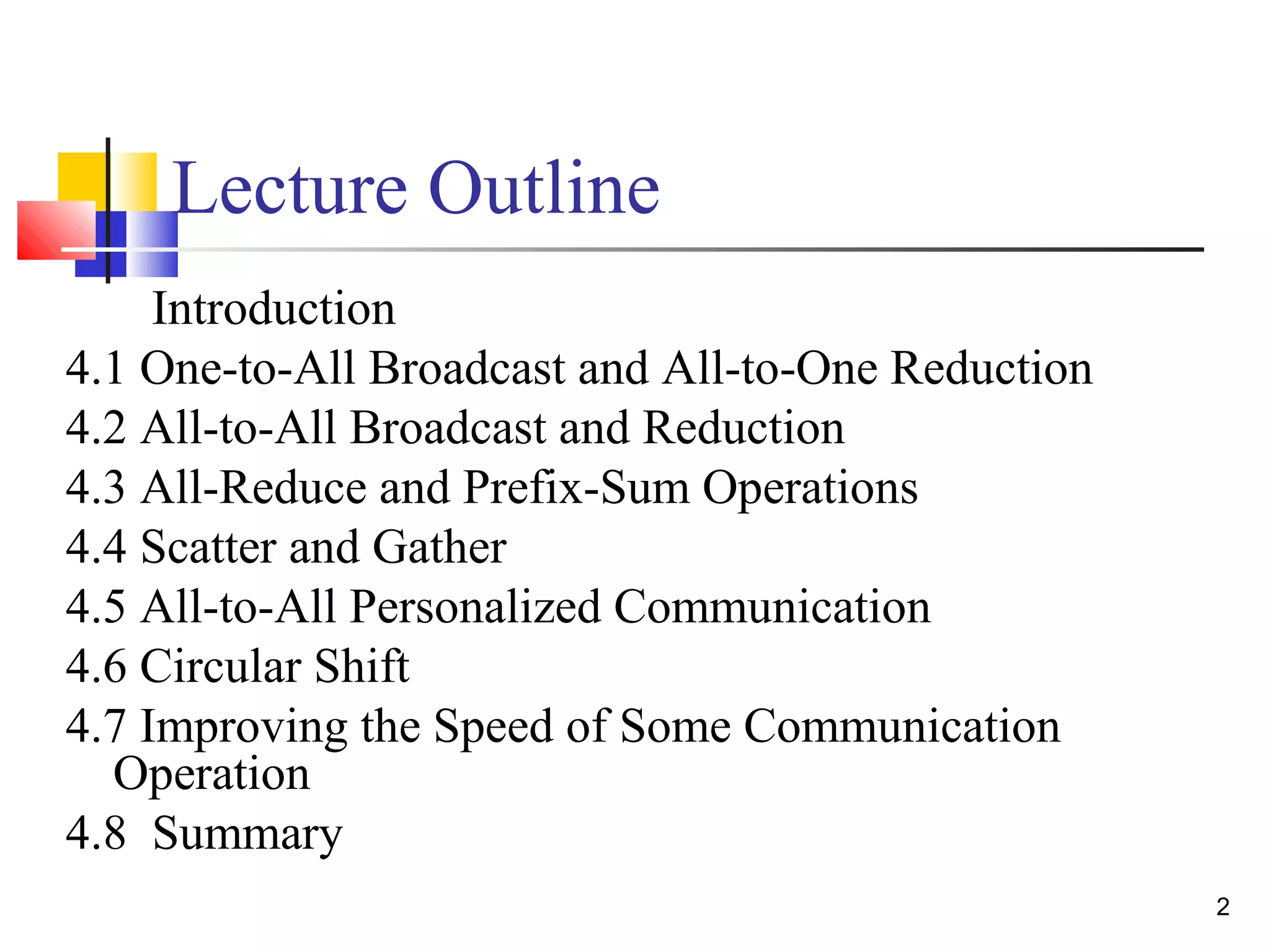
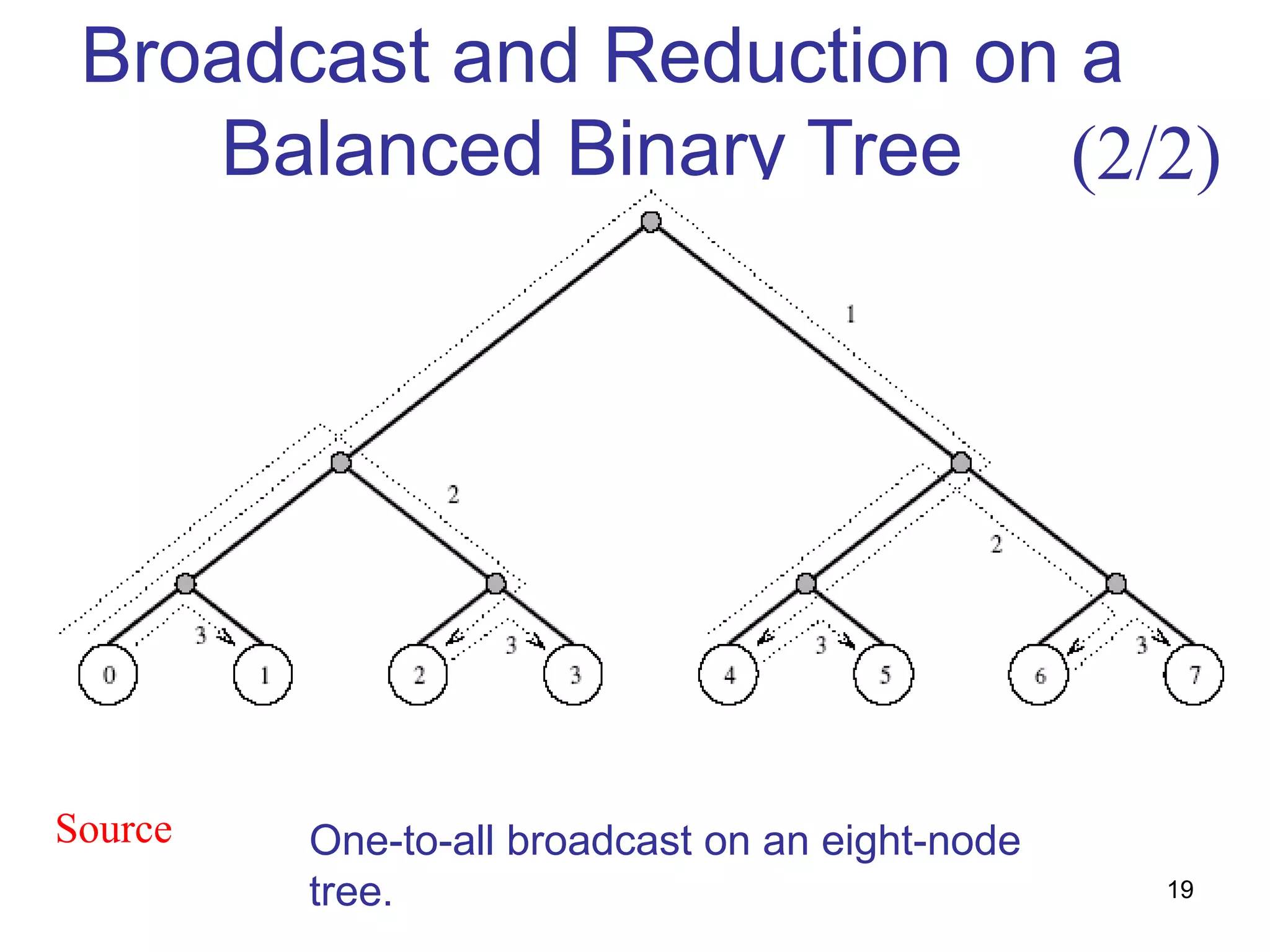
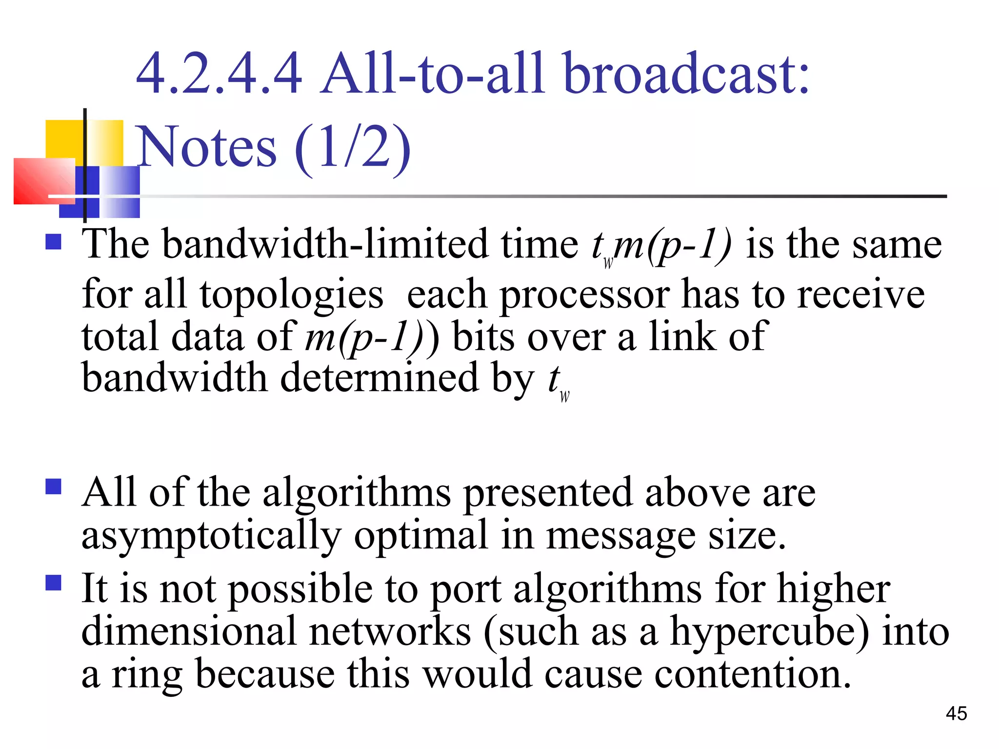
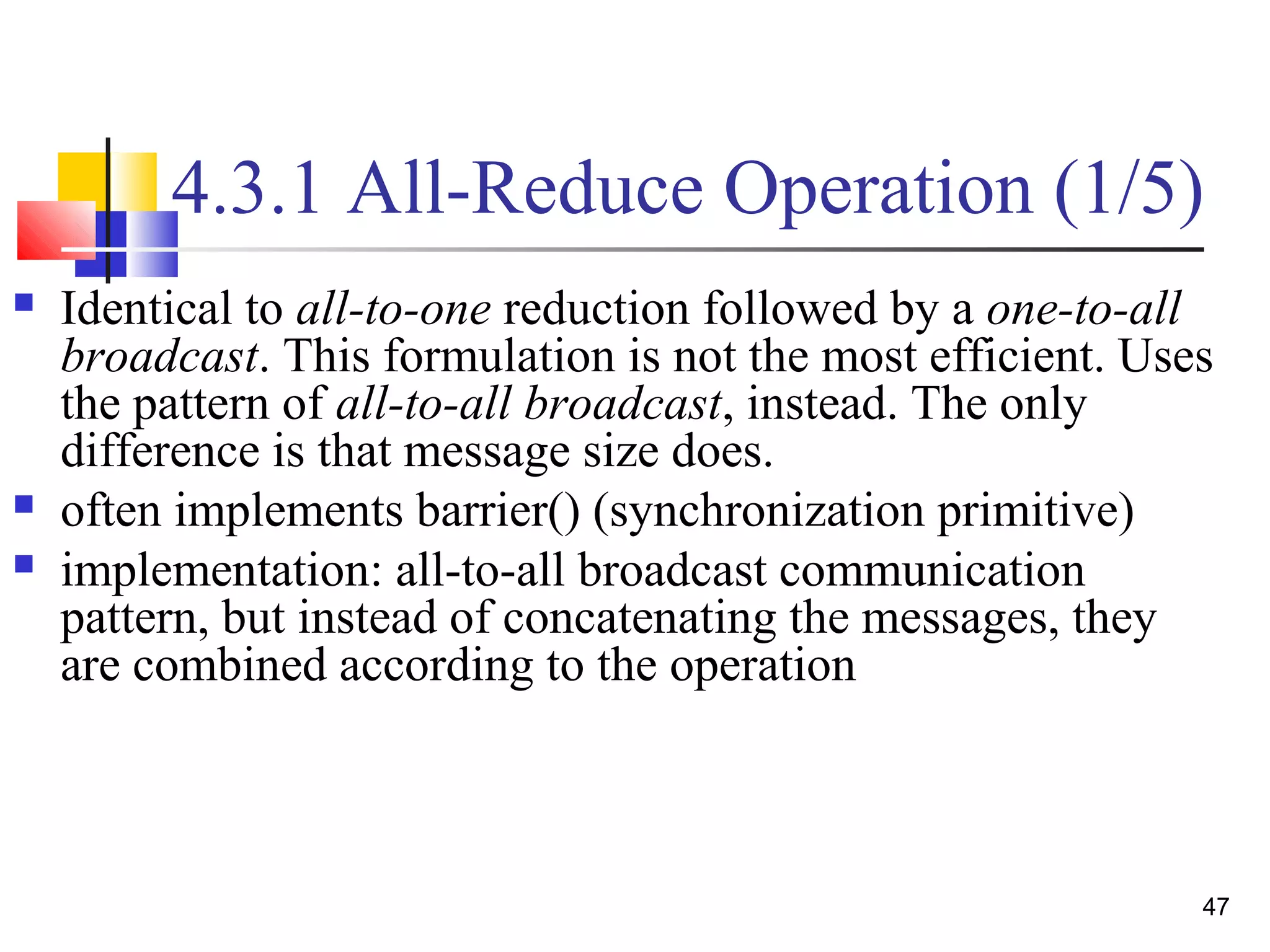
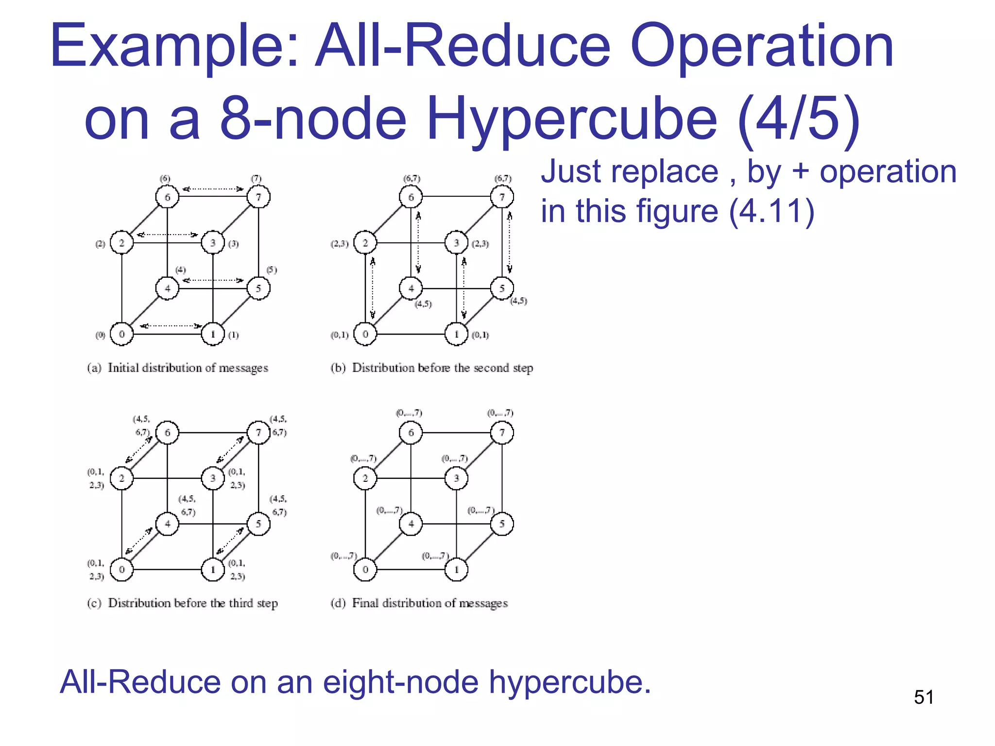
This document summarizes basic communication operations for parallel computing including: - One-to-all broadcast and all-to-one reduction which involve sending a message from one processor to all others or combining messages from all processors to one. - All-to-all broadcast and reduction where all processors simultaneously broadcast or reduce messages. - Collective operations like all-reduce and prefix-sum which combine messages from all processors using associative operators. - Examples of implementing these operations on different network topologies like rings, meshes and hypercubes are presented along with analyzing their communication costs. The document provides an overview of fundamental communication patterns in parallel computing.


![What is [Open] MPI?](https://cdn.slidesharecdn.com/ss_thumbnails/test-1230829557420508-1-thumbnail.jpg?width=640&height=640&fit=bounds)