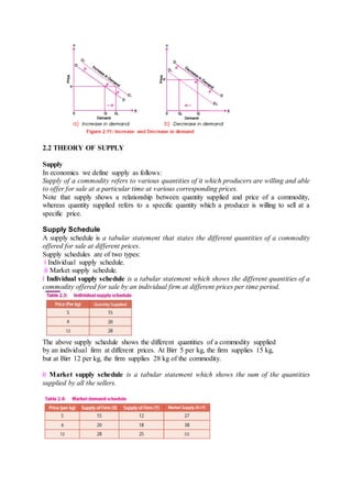
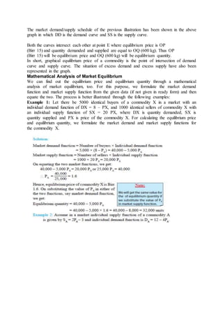
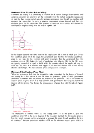
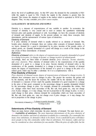
SlideShare a Scribd company logo
1 of 36
Chapter 2:- Demand, Supply and Elasticity
2.1 THEORY OF DEMAND
The words demand, desire and want are often interchangeably used to express what an
individual needs and what he would like to acquire. However, in economics, the term demand
has a specific meaning. It refers to the amount of commodity which an individual buyer is
willing and able to buy at a given price and during a given period of time. As such demand is
different from a mere desire. Human wants are unlimited, and therefore, desires are many.
But only a desire that is backed up by the capacity to pay the price for the commodity and the
willingness to buy it, is termed as a demand. We may say demand refers to an effective
desire. A desire becomes an effective desire or demand only when it is backed by the
following three factors:
 ability to pay for the good desired,
 willingness to pay the price of the good desired, and
 availability of the good itself.
Demand for a commodity is the amount of it that a consumer is willing to buy at various
given prices and a given moment of time.
Demand and quantity demanded are two different concepts. Whereas demand refers to the
relationship between the price of a commodity and its quantity demanded, other things being
same the quantity demanded refers to a specific quantity which a consumer is willing to buy
at a specific price.
Demand Schedule
A demand schedule is a tabular statement that states the different quantities of a commodity
that would be demanded at different prices. Demand schedules are of two types:
i Individual demand schedule.
ii Market demand schedule.
i Individual demand schedule is a tabular statement which shows the quantity of a
commodity demanded by an individual household at various alternate prices per time period.
The above demand schedule shows the different quantities of mangoes demanded
by an individual at different prices. At Birr 10 per kg consumer demands 4 kg
mangoes but at Birr 22 per kg consumer demands 1 kg mangoes.
ii Market demand schedule is a tabular statement which shows the different quantities of a
commodity demanded by different households or consumers in a market at various alternate
prices per time period.
The above demand schedule shows the different quantities of mangoes demanded
by different consumers at different prices. At Birr 10 per kg X demands 4 kg
whereas Y demands 6 kg, so market demand at Birr 10 per kg is 10 kg. But at
Birr 22 per kg X demands 1 kg whereas Y demands 2 kg, so market demand at
Birr 22 per kg is 3 kg.
Demand Curve
A demand curve conveys the same information as a demand schedule. But it shows the
information graphically rather than in a tabular form. Demand curves also are of two types
i Individual demand curve
ii Market demand curve
i Individual demand curve refers to the curve which expresses graphically the relationship
between different quantities of a commodity demanded by an individual at different prices
per time period.
The above demand curve shown in Figure 2.1 shows the different quantities of a
commodity demanded by an individual at different prices.
ii Market demand curve refers to the curve which express graphically the relationship
between different quantities of a commodity demanded by different households or consumers
at different prices per time period. It shows the demand of a whole market for a commodity.
The above market demand curve shows the horizontal summation of individual demand
curves. It expresses the relationship between different quantities of a commodity demanded
by X and Y at different prices. Market demand is obtained by horizontally summing
individual demands at each price.
Demand Function
All the above factors influencing the demand for a commodity can be briefly expressed in the
following functional relationship:
Dx = f (Px, Py, Pz, Y, T) (2.1)
Where, Dx stands for the demand for a commodity X,
Px shows the price of commodity X,
While Py and Pz refer to the prices of other substitutes and complementary goods. Y
represents the income level of the consumers, while T is an indicator of their tastes and
preferences. The word f shows the functional relationship between the demand for x and the
other variables Px, Py, Pz, Y, T etc. In simple words, this functional relationship shows that
the demand for commodity X depends upon the price of X, the prices of other goods, Y and
Z, the income of the consumers and their tastes and preferences.
Law of Demand
Law of demand expresses the functional relationship between the price of a commodity and
its quantity demanded. Price and demand are observed to be inversely related. In other words,
all other factors remaining constant, more of a commodity is demanded when price falls and
less of it is demanded when price rises, provided other factors remain the same. For example,
if the price of apples rises, people will buy less of them and vice-versa.
In Figure 2.3, we observe that when the price of apples is Birr 20 per kg, the demand is 2
kg. But when the price of apples falls to Birr 10 per kg, the demand for apples rises to 4 kg.
Statement of the Law:
The law of demand states that, other things being equal, at a higher price consumers will
purchase less of a commodity, and at a lower price, consumers will purchase more of it.
Or
A rise in the price of goods leads to a fall in quantity demanded and vice-versa, assuming all
other determinants of demand are kept constant.
Assumptions of the Law of Demand
Law of demand depends on the basic assumption of other things being equal (ceteris paribus).
By other things we mean factors other than price which affect the demand for a commodity.
For example, prices of related goods, tastes and preferences of consumer, income of the
consumer, population, etc. For the law to operate correctly, there should be no change in any
of these determinants.
We may summarize the assumptions of the law of demand as follows:
 There should be no change in prices of related goods,
 Tastes and preferences of the consumer should remain constant,
 There should be no change in the income of the consumers,
 The size of the population should remain constant,
 Distribution of income and wealth should be equal,
 There should be perfect competition in the market.
Exceptions to the Law of Demand
There are some situations when the law of demand does not operate. With an increase in
price, more quantity of a commodity is purchased and vice-versa. In these situations demand
curve is upward sloping. These are known as exceptions to the law of demand. Main
exceptions are as follows:
•• Giffen Goods: is a good for which an increase in the price raises the quantity demanded.
Economists use the term Giffen good to describe a good that violates the law of demand. (The
term is named for economist Robert Giffen, who first noted this possibility) Giffen goods are
very rare.
•• Prestige Goods: Some consumers measure the utility of a commodity entirely by its price.
For example diamond is considered as a prestige good in the society, the higher the price of
diamonds, the higher the prestige value of them. When the price of diamonds goes up their
prestige value will go up and, as a result, quantity demanded by consumers will rise.
•• Expectation of People about the Future: This assumption relates to the changes in the
expectations of the people regarding prices of the commodities in the future. For example, if
rainfall in any year does not occur in adequate quantity and there is widespread drought, the
expectations of the people will be that the prices would rise in the future. Therefore, even if
the prices of food grains are higher at present, they would demand greater quantities since
they will be expecting even higher prices in future.
•• Necessities: There are some commodities which are necessities of life – for example,
food grains, salt, medicines, etc. A minimum quantity of these commodities has to be
purchased by the consumer irrespective of their price. The law of demand does not hold good
in case of these commodities.
Basis of the Law of Demand Or Why Does the Demand Curve
Slope Downwards?
Demand curve normally slopes downwards to the right. It is also known as the negative slope
of the demand curve, indicating an inverse relationship between the price of the commodity
and its demand. There are several reasons for this inverse relationship as given below:
•• Law of diminishing marginal utility: According to this law, if a consumer increases the
consumption of a commodity in a given time period, the utility from consumption of each
successive unit goes on diminishing.
Due to this reason, the consumer will purchase the additional unit of commodity only when
he can pay less for it. Therefore, with a fall in price more units of a commodity will be
demanded and with a rise in price, fewer units of a commodity will be demanded.
•• Income effect: When the price of a commodity falls, a consumer can buy more of the
commodity with the same amount, indicating an increase in his real income. Similarly, a rise
in the price leads to a fall in real income of the consumer, and hence he buys less of a
commodity. This is called income effect.
•• Substitution effect: When the price of a commodity falls, it becomes relatively cheaper
than its substitutes. So people who are consuming the other goods would now start
consuming the commodity whose price has fallen, and as a result, its demand increases. This
increase in demand is called the substitution effect of price change.
•• Change in the number of consumers: A fall in the price of a commodity increases the
number of households who demand it in the market and a rise in the price of commodity
reduces this number.
•• Different uses of a commodity: At a lower price, a commodity will be in high demand
for being put to different uses. Conversely, at a higher price, its use will be limited to a few
essential uses only and hence the total demand will go down. For example, electricity could
be used for various purposes like lighting lamps, heating rooms and operating TV,
refrigerator, air conditioners etc. Suppose the price of electricity rises from Birr 1 per unit to
Birr 2 per unit. Then its consumption will be restricted to only essential purposes like the
lighting of lamps and operating of fans etc. As a result, the total demand for electricity will
decrease. On the other hand, a fall in the price of electricity will encourage its use for
different purposes and hence, the total demand for electricity will increase.
Determinants of Demand
An individual’s demand for a commodity is determined by a number of factors.
Some of these important factors are as follows:
•• Price of the Commodity: The price of a commodity is the most important factor which
affects the demand for a commodity. Other things remaining the same, if price increases,
quantity demanded decreases, and if price decreases, quantity demanded increases.
•• Income of the Consumer: Income of the consumer is also an important factor affecting
the demand for a commodity. Generally when income increases, demand also increases, and
when income decreases, demand also decreases. This is true in the case of normal goods.
However, in the case of inferior goods, with an increase in income their demand decreases
and vice-versa.
•• Prices of Related Goods: Changes in the prices of related goods also affect the demand
for a commodity. Related goods may be of two types:
 Substitute goods, and ‘Complementary goods.
 Substitute Goods: Substitute goods are those goods which can be used in place of
each other to satisfy a given want. That is why they are also called competitive
goods. Coffee and tea, pens and pencils, butter and oil, etc., are examples of
substitute goods.
 Complementary Goods: Complementary goods are those goods which are used
together to satisfy a given want. If two goods are complementary goods, a decline
in the price of one would directly change the demand for other commodity and
vice-versa. For example, cars and petrol are complements of each other. If the
price of car increases, its demand will decrease and thus will lead to a decrease in
the demand for petrol and vice-versa.
•• Tastes and Preferences: The amount demanded of a commodity also depends on
consumer tastes and preferences. If a consumer is accustomed to certain commodities, he will
demand that commodity and this leads to increase in the demand for that commodity.
•• Future Expectation of Changes in the Price: If there is an expectation of increase in the
price of a commodity in the near future, consumers will start demanding more of it. Contrary
to that, if the price of that commodity is likely to fall in near future, consumers will start
demanding less of that commodity.
•• Climate: The demand for a commodity is also affected by climate. For example, demand
for woolen clothes increases in cold seasons. On the other hand demand for coolers, cotton
clothes etc., increases in hot seasons.
•• Population and Number of Households: Changes in population or number of
households also affect the demand for goods. For example, with the increase in number of
households the demand for consumer goods will also increase.
•• Distribution of Income and Wealth: If the distribution of income and wealth in a society
is unequal, the demand for such commodities will be more which are generally demanded by
the rich people. On the other hand, if there is equal distribution of income and wealth in the
society, the demand for such commodity will be less which are specially used or demanded by
the rich people.
Demand mainly depends upon three factors, namely
 Price of the commodity;
 Income of the consumer, and
 Price of related goods.
On the basis of the above three factors, demand can be classified into three types:
i Price Demand,
ii Income Demand, and
iii Cross Demand.
Difference between Movement along a Demand Curve(or change in quantity demanded)
and Shift in the Demand Curve (or change in demand)
••Movement along a demand curve or change in quantity demanded:
Other things being equal, if the quantity demanded increases or decreases due to fall or rise
in the price of a commodity alone, it is known as movement along a demand curve or change
in quantity demanded. Here the movement is – either upward or downward – along the same
demand curve. Change in quantity demanded occurs due to change only in the price of the
commodity itself. Downward movement along the demand curve is called extension of
demand, while the upward movement as contraction of demand.
•• Shift in the demand curve or change in demand: If more or less of a commodity is
demanded, at the same price, due to change in factors other than the price of the commodity
concerned (such as change in income, or taste or prices of other related goods, etc.), it is
called shift in the demand curve or change in demand. In this situation, there is an either
rightward shift or leftward shift in the demand curve itself. Here the rightward shift in the
demand curve indicates increase in demand while the leftward shift indicates decrease in
demand.
2.2 THEORY OF SUPPLY
Supply
In economics we define supply as follows:
Supply of a commodity refers to various quantities of it which producers are willing and able
to offer for sale at a particular time at various corresponding prices.
Note that supply shows a relationship between quantity supplied and price of a commodity,
whereas quantity supplied refers to a specific quantity which a producer is willing to sell at a
specific price.
Supply Schedule
A supply schedule is a tabular statement that states the different quantities of a commodity
offered for sale at different prices.
Supply schedules are of two types:
i Individual supply schedule.
ii Market supply schedule.
i Individual supply schedule is a tabular statement which shows the different quantities of a
commodity offered for sale by an individual firm at different prices per time period.
The above supply schedule shows the different quantities of a commodity supplied
by an individual firm at different prices. At Birr 5 per kg, the firm supplies 15 kg,
but at Birr 12 per kg, the firm supplies 28 kg of the commodity.
ii Market supply schedule is a tabular statement which shows the sum of the quantities
supplied by all the sellers.
The above supply schedule shows the different quantities of a commodity supplied by
different firms at different prices. At Birr 5 per kg, firm X supplies 15 kg, whereas firm Y
supplies 12 kg, so market supply at Birr 5 per kg is 27 kg. But at Birr 12 per kg, firm X
supplies 28 kg, whereas firm Y supplies 25 kg. So market supply at Birr 12 per kg is 53 kg.
Supply Curve
A supply curve conveys the same information as a supply schedule. But it shows the
information graphically rather than in a tabular form.
Supply curves also are of two types:
i Individual supply curve.
ii Market supply curve.
i Individual supply curve refers to the curve which expresses graphically the relationship
between different quantities of a commodity supplied by an individual firm at different prices
per time period.
The above supply curve shows the different quantities of a commodity supplied by an
individual firm at different prices.
ii Market supply curve is found by adding horizontally the individual supply curves.
Figure 2.13: Indivdual and market supply curves
The above supply curve shows the horizontal summation of individual supply curves. It
expresses the relationship between different quantities of a commodity offered for sale by X
and Y at different prices. Market supply is obtained by horizontally summing individual
supplies at market price.
Supply Function
All the above factors influencing the supply of a commodity can be briefly expressed in the
following functional relationship:
SX = f(PX, PY, PF, B, Z) (2.5)
Where, SX stands for the supply of a commodity X and
PX shows the price of this commodity X, while PY is the price of related goods.
PF represents price of factors of production, B represents objectives of firm and Z refers to
other relevant factors. The world f shows the functional relationship between supply of X and
factors affecting its supply i.e., PX, PY, PF, B, Z etc.
Law of Supply
The Law of supply expresses the functional relationship between the price of a commodity
and its quantity supplied. Price and supply are observed to be directly related. In other words,
more of a commodity is supplied when price rises and less of it is supplied when price falls,
provided that other factors remain the same. For example, if the price of apples rises, quantity
supplied by sellers also rises and vice-versa.
In the above diagram, we observe that when the price of apples is Birr 10 per kg, the quantity
supplied is 1 kg. But when the price of apples rises to Birr 40 per kg, the quantity supplied
rises to 4 kg.
Statement of the Law
The law of supply states that there is a direct relationship between the price of a commodity
and its supply. Or other things being equal, the supply of a commodity increases with an
increase in its price and decreases with the fall in price.
Assumptions of the Law of Supply
Law of supply depends on the basic assumption, ‘other things being equal (ceteris paribus)’.
By other things we mean factors other than price which affect the supply of a commodity. For
example, price of related goods, price of factors of production, objectives of firm, production
technique etc. For the law, to operate there should be no change in any of these other
determinants. We may summarise the assumptions of the law of supply as follows:
 There should be no change in the prices of related goods,
 There should be no change in the prices of factors of production,
 There should be no change in the goals of the firm,
 There should be no change in the state of technology,
 The income of the buyers and sellers should remain constant.
Exceptions to the Law of Supply
There are some situations when the law of supply does not operate. With an increase in price,
less of a commodity is supplied and vice-versa. These are known as exceptions to the law of
supply. The main exceptions are as follows:
•• Future Expectations About Change in Prices: Law of supply will not apply if there is an
expectation about change in prices of a commodity in the near future.
•• Agricultural Products: The law of supply does not apply in the case of agricultural
products because their supply is governed by natural factors such as flood, drought, rainfall
etc.
•• Perishable Commodities: The supply of perishable commodities like milk, fruits,
vegetables etc. is not affected by their prices. Producers try to sell more perishable
commodities even when their prices decline.
•• Good of Auction: Since supply of auction goods is limited, the law of supply does not
operate in their case.
•• Artistic Goods: Law of supply does not apply in the case of artistic goods since the
supply of these goods cannot be changed.
Basis of the Law of Supply or Why does the Supply Curve Slope Upwards?
A supply curve normally slopes upwards to the right. It is also known as the positive slope of
the supply curve, indicating a direct relationship between the price of the commodity and its
supply. There are several reasons for this direct relationship, as given below:
•• Expectations of Profit: If prices are high, profit expectation increases with the result
that producers increase their output or production.
Conversely, if the prices are low, profit expectation reduces with the result that producers
reduce their output or production.
•• Change in Stock: An increase in the price of a commodity induces the sellers to dispose
of at least a part of their stock. Conversely, if there is a decrease in the price of the
commodity, sellers retain some of the stocks.
•• Entry and Exit of Firms: If, due to rising prices there are high profits, new firms enter
into the market and add to the supply of the commodity. Conversely, if there is a decline in
price or loss, inefficient firms withdraw from the market and stop producing that commodity.
Determinants of Supply
Supply of a commodity is determined by a number of factors. Some of these important
factors are as follows:
•• Price of the Commodity: The price of a commodity is the most important factor affecting
its supply. Generally, the relationship between price and quantity supplied is direct – i.e.,
supply is more when price is more and vice-versa.
•• Changes in Factor Prices: Change in factor prices have a strong influence on the supply
of a good in the market. An increase in the prices of factors of production leads to an
increase in the cost of production. As a result the producers will not be able to sell the same
amount at the prevailing market prices. Since their production cost has gone up, the only way
the same amount can be offered is at a higher price.
•• Price of Related Goods: An increase in the price of other, related goods induces the
firms to produce more of those other goods, leading to a reduction in the supply of the goods
whose price has remained unchanged.
•• Objectives of the Firm: Generally, the main objective of a firm is to maximise its profit.
Profit is maximum when the difference between income and expenditure is maximum.
However, besides this objective there are other objectives which a firm may pursue, such as
objectives of maximum sales, maximum employment, more production, etc. In such a
situation, if a firm aims at some other objective such as more employment besides the
objective of maximum profit, then volume of output or supply will increase, even when profit
declines.
•• State of Technology: If there is change in the technique of production leading to fall in
the cost of production, supply of a commodity will increase. On the other hand, supply of
those commodities will be less whose production depends on old technology.
•• Other Factors: Beside the main factors discussed above, there are many other factors
which affect the supply of a commodity such as fiscal policy of the government, the prices
which are likely to prevail in the near future, etc.
(or change in Quantity Supplied) and Shift in the Supply
Curve (or change in Supply)
•• Movement along a supply curve (or change in quantity supplied): Other things being
equal, if the quantity supplied increases or decreases due to rise or fall in the prices of the
commodity alone, it is known as movement along a supply curve or change in quantity
supplied. In this, we move along the same supply curve either upwards or downwards.
Upward movement along the supply curve is extension of supply (that is, more quantity
supplied at a higher prices) while the downward movement is contraction of supply (that is,
less quantity supplied at a lower prices).
•• Shift in the supply curve (or change in supply): If more or less quantity of a commodity
is supplied at every alternative price due to changes in factors other than the price of the
commodity concerned, it is known as shift in the supply curve or change in supply. In this
situation, supply curve itself shifts either to right or to the left. Rightward shift of supply
curve indicates increase in supply, while leftward shift indicates decrease in supply.
Thus, movement along the supply curve is caused by a change in the commodity’s own price.
In this situation, supply curve remains the same. On the other hand, a shift in the supply curve
is caused by a change in something other than the commodity’s own price. A shift in the
supply curve may be caused by change in the prices of other goods, change in the prices of
factors of production, change in technique of production or change in the goals of the
producer.
2.3 MARKET EQUILIBRIUM
In previous sub-units, we have discussed consumers’ demand for goods in a market and
firms’ supply of goods in a market separately. Demand and supply producers supply at
different prices. But they do not tell us what the actual price of a good will be. We now come
to the important question: How do the forces of demand and supply interact to determine
market prices? We explain how forces of demand and supply help in attaining ‘equilibrium’,
and how the ‘equilibrium price’ is determined. We also consider the effects of shifts in
demand and supply on the equilibrium price, in this sub-unit.
The Concept of Equilibrium
In the methodologies of economics, the concept of equilibrium occupies an important place.
It is employed in almost every theory of economics in the fields of price, income, and growth.
The word equilibrium means a state of balance. In the physical world, when two opposing
forces that impinge on an object are in balance, and the object is held still by them, the object
is said to be in equilibrium. In other words, when the object under the pressure of forces
working in opposing directions has no tendency to move in either direction, the object is in
equilibrium. In the same way, a system is said to be in equilibrium when its important
variables show no change, and when no forces are acting on them to change their values. For
example, upon reaching equilibrium, a consumer has no inclination to re-allocate his or her
money expenditure. Similarly, a firm is said to be in equilibrium when it has no tendency to
change its level of output by either increasing or contracting it.
In actual economic activities, equilibrium may never be actually realised. The central feature
of equilibrium analysis in economics is the concept that economies tend toward equilibrium
when no new forces are acting on them.
Market Equilibrium
In the context of price determination, equilibrium refers to a situation in which the quantity
demanded of a commodity equals the quantity supplied of the commodity.
It refers to the balance between opposite forces of demand and supply and is termed as
market equilibrium.
Equilibrium Price
The price at which the quantity demanded of a commodity equals quantity supplied is known
as ‘equilibrium price’. The price of commodity in a market is determined by its demand and
supply. At equilibrium price, demand and supply are in equilibrium.
Equilibrium Quantity
The equilibrium price is the price at which the consumers are willing to purchase the same
quantity of a commodity which producers are willing to sell. The amount that is bought and
sold at equilibrium price is called the ‘equilibrium quantity’.
Market Equilibrium – An Illustration
With a view to understanding how the forces of demand and supply operate in a market to
determine an equilibrium price and quantity, let us consider an imaginary market having a
large number of buyers and sellers of a commodity, say oranges.
Table 2.5 shows the imaginary market’s demand/supply schedule of oranges at different
prices.
In the above schedule there is one price at which market demand is equal to market supply.
This price is Birr 15 per kg because, at this price, quantity demanded is equal to quantity
supplied, that is, 600 kg of oranges. Thus equilibrium price is determined as Birr 15 per kg. It
is the only price at which the maximum number of buyers and sellers are satisfied. So long as
market demand and supply remain unchanged, the price will neither tend to rise nor fall
below this equilibrium price.
In Case of Excess Demand
Excess demand for a product means that the consumers want more than what the producers
are willing to supply. If at a given price of a commodity, demand is in excess of supply,
competition among buyers will push the price up to the point at which demand becomes
equal to supply. Suppose the actual price of oranges prevailing at a particular time in the
market is Birr 10 per kg. At this price, demand for oranges is for 800 kg, whereas supply is
400 kg, that is, there is excess demand of 400 (= 800 – 400) kg. This will create competition
among buyers to buy oranges which are in short supply and push the price up till it reaches
the equilibrium price of Birr 15 per kg, where demand becomes equal to supply (= 600 kg of
oranges).
In Case of Excess Supply
Excess supply of a product means that the consumers want less than what the producers are
willing to supply. If at a given price, the quantity supplied of a commodity exceeds the
quantity demanded, competition among sellers will push the price down to the point at which
demand becomes equal to supply. Suppose at a particular time, price of oranges prevails at
Birr 20 per kg at which the demand is for 400 kg against a supply of 800 kg, i.e., there is
excess supply of 400 kg. Competition among sellers to sell their oranges will push down the
price till it reaches Birr 15 per kg. Ultimately the price will settle at Birr 15 per kg at which
demand is 600 kg oranges and supply is also 600 kg. This indicates demand and supply are
holding each other in balance and the equilibrium price has been reached. Note that in the
above illustration, the equilibrium price is Birr 15 per kg and the equilibrium quantity is 600
kg.
Graphical Presentation of Market Equilibrium
Determination of equilibrium price and equilibrium quantity can also be illustrated
graphically with the help of a market demand curve and market supply curve.
The market demand/supply schedule of the previous illustration has been shown in the above
graph in which DD is the demand curve and SS is the supply curve.
Both the curves intersect each other at point E where equilibrium price is OP
(Birr 15) and quantity demanded and supplied are equal to OQ (600 kg). Thus OP
(Birr 15) will be equilibrium price and OQ (600 kg) will be equilibrium quantity.
In short, graphical equilibrium price of a commodity is the point of intersection of demand
curve and supply curve. The situation of excess demand and excess supply have also been
represented in the graph.
Mathematical Analysis of Market Equilibrium
We can find out the equilibrium price and equilibrium quantity through a mathematical
analysis of market equilibrium, too. For this purpose, we formulate the market demand
function and market supply function from the given data (if not given in ready form) and then
equate the two. The process is better illustrated through the following examples:
Example 1: Let there be 5000 identical buyers of a commodity X in a market with an
individual demand function of DX = 8 – PX, and 1000 identical sellers of commodity X with
an individual supply function of SX = 20 PX, where DX is quantity demanded, SX is
quantity supplied and PX is price of the commodity X. For calculating the equilibrium price
and equilibrium quantity, we formulate the market demand and market supply functions for
the commodity X.
Demand and Supply Curves do not Intersect each other –
Is it possible?
A situation may arise when there are prospective consumers and producers of a commodity
but still it is not produced. Why? It happens when the price at which producers are ready to
produce is so high that the consumers are not willing to buy even a single unit of the
commodity. In other words, in graphic terms, the demand curve and supply curve do not
intersect each other at any positive quantity. As a result the product will not be produced.
This shows the industry (of the product) is not economically viable.
Thus a non-viable industry is one whose demand and supply do not intersect each other at
any positive quantity. It is an industry in which costs are too high for any positive output to
be produced.
Effects of Government Intervention on Market Equilibrium
Government may intervene in the market in many ways; one of the more prominent ways is
of price control. In the interest of consumers and producers, the government executes the
policy of price control by intervening in the market.
This policy of price-control may have two variants:
 maximum price and
 minimum price.
In both the situations decisions are taken on the basis of demand and supply analysis.
Maximum Price Fixation (Price Ceiling)
Sometimes the supply of a commodity is so short that it creates shortages in the market and
common consumers are unable to get the commodity from the market. Competitive prices are
so high that they become out of reach for common consumers, only the rich can purchase and
consume the commodity. In such a situation government comes forward and fixes the
maximum price for the commodity. This process is known as price ceiling. We discuss the
consequences of price ceiling with the help of Figure 2.26.
In the diagram demand curve DD intersects the supply curve SS at point E which gives OP as
the equilibrium price. If at this stage, the government feels that this free market equilibrium-
price is too high for the common and poor consumers then the government fixes the
maximum price at OP1 below the level of equilibrium price (that is, OP). At this OP1 price
the quantity demanded is equal to OQ1 while the quantity offered for supply will only be
equal to OQ. Thus, it is revealed that supply is less than the demand and it leads to the
situation of shortages. We may conclude, price ceiling causes shortages.
Minimum Price Fixation (Price Floor)
Whenever government feels that the competitive price determined by the forces of demand
and supply in a free market is not fair from the producers’ point of view, government
announces a minimum price to protect the interests of the producers. This is also termed as
support price or price floor. It is very common with governments these days to protect the
interests of the farmers. We discuss the consequences of price floor with the help of Figure
2.27.
The intersection of demand curve DD and supply curve SS at the point E, gives the
equilibrium price OP in the above diagram. If the producers feel that this free market price is
low, they exert pressure on the government to enhance this price through legislation. In view
of producers’ interests government declares OP1 as the minimum support price, which is
above the level of equilibrium price. At this OP1 price the demand for the commodity is OQ1
while the supply is equal to OQ. Clearly the supply in this situation is greater than the
demand. This creates the situation of surplus in the market which is equivalent to M1M in the
diagram. Thus, we may conclude price floor causes surplus.
2.4 ELASTICITY OF DEMAND AND SUPPLY
Elasticity is a measure of responsiveness of one variable to another. In economics, the
concept of elasticity is very crucial and is used to analyse the quantitative relationship
between price and quantity purchased or sold. Accordingly, we have the concepts of elasticity
of demand and elasticity of supply. In the present subunit, we study these concepts, their
determinants and the measurement of various types of elasticities.
Elasticity of Demand
It is price elasticity of demand which is usually referred to as elasticity of demand. But,
besides price elasticity of demand, there are various other concepts of demand elasticity. As
we know, demand for a good is determined by its price, incomes of the people, prices of
related goods, etc. Quantity demanded of a good will change as a result of the change in the
size of any of these determinants of demand.
Definition:
Elasticity of demand refers to the degree of responsiveness of quantity demanded of a good
to a change in its price, or change in income, or change in prices of related goods.
Accordingly, there are three kinds of demand elasticity: price elasticity, income elasticity,
and cross elasticity. Price elasticity of demand refers to the responsiveness of the quantity
demanded of a good to a change in its price. Income elasticity of demand refers to the
sensitiveness of the quantity demanded to a change in income. Cross elasticity of demand
means the degree of responsiveness of the demand of a good to a change in the price of a
related good, which may be either a substitute for it or a complementary with it.
Price Elasticity of Demand
Price elasticity of demand means degree of responsiveness of demand to change in price. It
indicates how consumers react to changes in price. The greater the reaction, the greater will
be the elasticity, and the lesser the reaction, the smaller will be the elasticity. Price elasticity
of demand is a measure of how much the quantity demanded of a good responds to a change
in the price of that good, computed as the percentage change in quantity demanded divided
by the percentage change in price. For example, demand for commodities like clothes, fruit
etc. changes when there basic necessities of life, like salt, food grains etc., may not change
even if price changes, or it may change, but not in proportion to the change in price. is even a
small change in their price, whereas demand for commodities which are basic necessities of
life, like salt, food grains etc., may not change even if price changes, or it may change, but
not in proportion to the change in price.
Determinants of Price Elasticity of Demand
There are many factors which determine the price elasticity of demand. The main factors are:
•• Availability of substitutes: The most important determinants of the price elasticity of
demand is the number and kind of substitutes available for a commodity. If a commodity has
many close substitutes, its demand is likely to be elastic. Even a small fall in price will induce
more people to buy this commodity rather than its substitutes. For instance, coffee and tea
may be considered as close substitutes for one another. When the price of coffee falls, but the
price of tea does not, many consumers will buy more coffee and less of tea since coffee has
become relatively cheap. On the other hand, if a good has no or weak substitutes, the demand
for it would be inelastic. This is the case with milk, salt and sugar which do not have good
substitutes. Thus, when the price of milk increases, the quantity demanded will not decrease
much, and, similarly, when the price falls, the quantity demanded will not increase much. In
general, a commodity with close substitutes tends to have an elastic demand, and one with
weak substitutes has an inelastic demand.
•• Nature of the commodity: One of the important determinants of price elasticity of
demand is nature of the commodity, that is, whether it is a ‘necessary’ or a ‘luxury’ or a
commodity of ‘comfort’. Demand for necessities, such as food items, is generally inelastic.
These goods are essential for existence. On the other hand, ‘luxuries’ and ‘comforts’ are not
essential for existence and their consumption can be dispensed with or postponed. Thus, their
demand changes by large amounts due to small changes in price. For example, a fall in the
price of air conditioners, colour TV sets, and so forth may bring about a large increase in the
quantities demanded of these goods. Generally the demand for necessities is inelastic and the
demand for luxuries and comforts is elastic.
•• Proportion of income spent: Elasticity of demand for a commodity depends upon the
proportion of her/his income which the consumer spends on it. The smaller the proportion of
income spent on a commodity, the smaller will be the elasticity of demand and vice-versa.
The demand for soap, salt, matches, etc., is highly inelastic since the consumer spends a very
small proportion of his income on them. On the other hand, the demand for clothes, furniture,
etc. is likely to be elastic since the consumer spends a large fraction of his income on these
goods.
•• The number of uses of a commodity: Elasticity of demand depends also upon the
number of uses a commodity can be put to. The greater the number of uses to which a
commodity can be put to, the greater will be its price elasticity of demand. Electricity, for
example, can be used for lighting, cooking, heating, etc. If electricity is very expensive, it
might be used for lighting only. As the price of electricity falls, it might be used for less
important uses like cooking and heating. Accordingly, the demand for electricity will change
greatly with a change in its price and, therefore, it is relatively elastic.
•• Time factor: The elasticity of demand depends on the size of the time period – short
period or long period. Price elasticity is generally low for short periods as compared to long
periods. This is for two reasons.
Firstly, it takes time for consumers to adjust their tastes, preferences and habits. Secondary,
new substitutes may be developed in the long run. Therefore, if the price of a commodity
rises, the demand for it will be inelastic in the short-run as the substitutes may not be
available. But in the long-run, demand will be elastic as the consumers may switch over to
new substitute.
•• Postponement of consumption: Elasticity of demand depends on the possibility of
postponement of consumption as well. Demand for a commodity is elastic if its consumption
can be postponed. The consumption of clothing may be postponed and, therefore, a rise in its
price may lead to a large fall in its demand. But the consumption of food items cannot be
postponed. Therefore, their demand is inelastic.
•• Price range: Price elasticity of demand depends upon the range of prices. Demand for a
commodity tends to be inelastic at very high and very low prices, and elastic within the
moderate range of prices. At a very high price of the commodity, the demand for it will come
from rich persons only. A rise or fall in its price will not affect its demand much, as it would
still be out of reach for most of the people. If, on the other hand, the price of the commodity is
very low, all those who want to buy it would have already purchased this commodity. A
further fall in the price of the commodity, therefore, will not lead to much increase in amount
demanded. However, the demand for the commodity is elastic within the moderate range of
prices, as the commodity will be within the reach of a large number of consumers.
•• Habits of the consumers: Price elasticity of demand depends also upon whether or not
the consumers are in the habit of using a commodity. If consumers are in the habit of
consuming some commodities, they will continue to consume them even at higher prices. For
instance, a smoker does not reduce much the number of cigarettes smoked as the price of
cigarettes goes up. The demand for such commodities is usually inelastic.
Measurement of Price Elasticity of Demand
The measurement of elasticity of demand can be looked at from two view points:
i point elasticity and
ii arc elasticity.
i Point Elasticity: When price elasticity of demand is measured at a point on a demand
curve, it is called point elasticity. In the following Figure 2.28 if we want to know the
elasticity of demand at a point R on the demand curve, we call it point elasticity. The method
used for measuring point elasticity is called Point Method.
Figure 2.28: Point and arc elasticities
ii Arc Elasticity: When elasticity of demand is measured over a finite range or ‘arc’ of a
demand curve, it is called arc elasticity of demand. For example, the measure of elasticity
between point R and R1 on the demand curve is the measure of arc elasticity.
Remember that we ignore the minus sign when calculating price elasticity. Mathematically
speaking, price elasticity of demand is a negative number because of negative slope of the
demand curve. In view of the negative slope from each other. Thus, while calculating price
elasticity of demand by percentage method, the common practice is to ignore the negative
signs, i.e., we should take only the absolute values and not their signs.
Another important feature of the price elasticity of demand is that it does not depend on the
units of measurement of quantity of demand – whether kg of rice or litres of petrol – or the
measure of price – whether in Ethiopian Birr or in U.S. dollars. It is a unit-free measure.
Therefore, we can compare the price sensitivity of demand for different goods regardless of
the units for measuring either price or quantity.
Let us calculate elasticity of demand by using the point method by taking a numerical
example. Suppose the price of the commodity falls from Birr 5 to Birr 4 and quantity
demanded increases from 100 units to 150 units. In this example; Given: Q1 = 100, Q2 = 150,
P1 = 5, P2 = 4
Cross Elasticity of Demand
Responsiveness in the demand for a commodity to the changes in the prices of its related
goods is called cross elasticity of demand. In other words cross elasticity of demand may be
defined as the ratio of proportionate change in the demand of one commodity (say x) to the
proportionate change in the price of another commodity (say y). It can be measured as
follows:
2.5 ELASTICITY OF SUPPLY
Price Elasticity of Supply
Price elasticity of supply to change in price, indicates how sellers react to change
in price. The greater the reaction, the greater will be the elasticity, lesser the
reaction, the smaller will be the elasticity.
For example, if the price of wheat rises, the farmers may be tempted to sell more
in the market, and keep less for themselves. On the other hand, if the price of cars
rises, the car manufacturers may not probably be in a position to offer more cars
for sale, because they may not be keeping stock of cars.
Determinants of Price Elasticity of Supply
There are many factors which determine the price elasticity of supply. The main factors are:
•• Behaviour of cost of production: Elasticity of supply depends upon change in the cost of
producing additional quantity of output. If an increase in output by the firms in an industry
causes only a slight increase in their cost per unit or leads to a decrease in cost per unit, we
would expect supply to be fairly elastic. If, on the other hand, an increase in supply leads to a
large increase in cost of production, the supply would be relatively inelastic.
•• Time element: A price change due to change in demand for a commodity may have a
small response in the quantity supplied in the short-run since the production capacity may be
limited. Therefore, in the shortrun, supply tends to be relatively inelastic. However, in the
long-run, new plants can be set up and production capacity can be expanded.
Therefore, in the long-run supply tends to be elastic.
•• Nature of the commodity: Nature of the commodity is also an important determinant of
the elasticity of supply. For instance, the supply of durable products is relatively elastic.
Durable goods can be stored and hence producers can meet the market demand by running
down their stocks. Therefore, supply of such goods can be increased or decreased quickly in
response to change in price. On the other hand, supply of perishable goods like milk and
vegetables is relatively less elastic.
•• Availability of facilities for expanding output: The response of producers to changes in
price depends on the availability of production facilities. If producers have sufficient
production facilities, such as availability of raw materials, power, etc. they would be able to
increase their supply in response to rises in prices of the commodities. The supply, therefore,
will be elastic. But if, on the other hand, there is shortage of power, fuel and essential raw
materials, the output would expand slowly in response to rises in prices of the commodities.
•• Nature of inputs: Elasticity of supply depends on the nature of inputs used for the
production of a commodity. If the production of a product requires inputs that are easily
available, its supply would be more elastic. On the other hand, if it uses specialised inputs, its
supply will be relatively inelastic.
•• Risk-taking: The elasticity of supply is determined by the willingness of the
entrepreneurs to take risk. If entrepreneurs are willing to take risk, the supply will be more
elastic. On the other hand, if entrepreneurs hesitate to take risks, the supply will be inelastic.
•• Expectation of future prices: If the producers expect a rise in the price of a commodity
in future, producers will like to hoard the commodity to take advantage of rise in future price.
The supply will, therefore, be less elastic. On the other hand, if they expect a fall in future
price, they will release the goods from their stocks. The supply will be more elastic.
Measurement of Price Elasticity of Supply
As the case with price elasticity of demand, we can measure the price elasticity of supply
using different methods. However, a simple and most commonly used method is point
method.
Point Method: The point method of measuring the price elasticity of supply is based on the
definition of elasticity, that is, the ratio of proportionate change in quantity supplied of a
commodity to a given proportionate change in its price.
Thus, the formula for measuring price elasticity of supply is:
Chapter 2 Demand and Supply.docx

More Related Content

Similar to Chapter 2 Demand and Supply.docx

Demand, Supply 2009 1
Demand, Supply 2009  1Demand, Supply 2009  1
Demand, Supply 2009 1siraj2762268
 
Chapter-2.new.ppt
Chapter-2.new.pptChapter-2.new.ppt
Chapter-2.new.pptManojMba2
 
Presentation on demand & supply
Presentation on demand & supplyPresentation on demand & supply
Presentation on demand & supplyVikash Barnwal
 
presentation_demand_&_supply_1453886502_164314.pptx
presentation_demand_&_supply_1453886502_164314.pptxpresentation_demand_&_supply_1453886502_164314.pptx
presentation_demand_&_supply_1453886502_164314.pptxRajeshKumar965860
 
Theory of demand
Theory of demandTheory of demand
Theory of demandNitin Setia
 
CA NOTES ON THEORY OF DEMAND AND SUPPLY IN BUSINESS ECONOMICS
CA NOTES ON THEORY OF DEMAND AND SUPPLY IN BUSINESS ECONOMICSCA NOTES ON THEORY OF DEMAND AND SUPPLY IN BUSINESS ECONOMICS
CA NOTES ON THEORY OF DEMAND AND SUPPLY IN BUSINESS ECONOMICSKanoon Ke Rakhwale India
 
Elasticity of demand
Elasticity of demandElasticity of demand
Elasticity of demandSVGANGAD
 
Demand and supply by kushal devda
Demand and supply by kushal devdaDemand and supply by kushal devda
Demand and supply by kushal devda7799220766
 
Economics 2.pdf
Economics 2.pdfEconomics 2.pdf
Economics 2.pdfFraolUmeta
 
L of demand converted
L of demand convertedL of demand converted
L of demand convertedDiptiSingh55
 
Law of Demand and Supply equilibrium supply curve and demand curve (1).pptx
Law of Demand and Supply equilibrium supply curve and demand curve (1).pptxLaw of Demand and Supply equilibrium supply curve and demand curve (1).pptx
Law of Demand and Supply equilibrium supply curve and demand curve (1).pptxJoshuaAsucro
 
UNIT 1 MICROECONOMICS.pptx
UNIT 1 MICROECONOMICS.pptxUNIT 1 MICROECONOMICS.pptx
UNIT 1 MICROECONOMICS.pptxMonishBalaji8
 
demand and its determinants
demand and its determinantsdemand and its determinants
demand and its determinantsSakshi Agarwal
 

Similar to Chapter 2 Demand and Supply.docx (20)

Demand.pdf
Demand.pdfDemand.pdf
Demand.pdf
 
Demand
DemandDemand
Demand
 
Demand, Supply 2009 1
Demand, Supply 2009  1Demand, Supply 2009  1
Demand, Supply 2009 1
 
Chapter-2.new.ppt
Chapter-2.new.pptChapter-2.new.ppt
Chapter-2.new.ppt
 
demand.pptx
demand.pptxdemand.pptx
demand.pptx
 
Presentation on demand & supply
Presentation on demand & supplyPresentation on demand & supply
Presentation on demand & supply
 
presentation_demand_&_supply_1453886502_164314.pptx
presentation_demand_&_supply_1453886502_164314.pptxpresentation_demand_&_supply_1453886502_164314.pptx
presentation_demand_&_supply_1453886502_164314.pptx
 
Theory of demand
Theory of demandTheory of demand
Theory of demand
 
Economics of Demand & Supply
Economics of Demand & SupplyEconomics of Demand & Supply
Economics of Demand & Supply
 
CA NOTES ON THEORY OF DEMAND AND SUPPLY IN BUSINESS ECONOMICS
CA NOTES ON THEORY OF DEMAND AND SUPPLY IN BUSINESS ECONOMICSCA NOTES ON THEORY OF DEMAND AND SUPPLY IN BUSINESS ECONOMICS
CA NOTES ON THEORY OF DEMAND AND SUPPLY IN BUSINESS ECONOMICS
 
Elasticity of demand
Elasticity of demandElasticity of demand
Elasticity of demand
 
Demand and supply by kushal devda
Demand and supply by kushal devdaDemand and supply by kushal devda
Demand and supply by kushal devda
 
Demand analysis
Demand analysisDemand analysis
Demand analysis
 
Economics 2.pdf
Economics 2.pdfEconomics 2.pdf
Economics 2.pdf
 
Demand analysis
Demand analysisDemand analysis
Demand analysis
 
L of demand converted
L of demand convertedL of demand converted
L of demand converted
 
Law of Demand and Supply equilibrium supply curve and demand curve (1).pptx
Law of Demand and Supply equilibrium supply curve and demand curve (1).pptxLaw of Demand and Supply equilibrium supply curve and demand curve (1).pptx
Law of Demand and Supply equilibrium supply curve and demand curve (1).pptx
 
Demand final
Demand finalDemand final
Demand final
 
UNIT 1 MICROECONOMICS.pptx
UNIT 1 MICROECONOMICS.pptxUNIT 1 MICROECONOMICS.pptx
UNIT 1 MICROECONOMICS.pptx
 
demand and its determinants
demand and its determinantsdemand and its determinants
demand and its determinants
 

Recently uploaded

Turn Lock Take Key Storyboard Daniel Johnson
Turn Lock Take Key Storyboard Daniel JohnsonTurn Lock Take Key Storyboard Daniel Johnson
Turn Lock Take Key Storyboard Daniel Johnsonthephillipta
 
Gomti Nagar & High Profile Call Girls in Lucknow (Adult Only) 8923113531 Esc...
Gomti Nagar & High Profile Call Girls in Lucknow  (Adult Only) 8923113531 Esc...Gomti Nagar & High Profile Call Girls in Lucknow  (Adult Only) 8923113531 Esc...
Gomti Nagar & High Profile Call Girls in Lucknow (Adult Only) 8923113531 Esc...gurkirankumar98700
 
FULL ENJOY - 9953040155 Call Girls in Moti Nagar | Delhi
FULL ENJOY - 9953040155 Call Girls in Moti Nagar | DelhiFULL ENJOY - 9953040155 Call Girls in Moti Nagar | Delhi
FULL ENJOY - 9953040155 Call Girls in Moti Nagar | DelhiMalviyaNagarCallGirl
 
FULL ENJOY - 9953040155 Call Girls in Gtb Nagar | Delhi
FULL ENJOY - 9953040155 Call Girls in Gtb Nagar | DelhiFULL ENJOY - 9953040155 Call Girls in Gtb Nagar | Delhi
FULL ENJOY - 9953040155 Call Girls in Gtb Nagar | DelhiMalviyaNagarCallGirl
 
Hazratganj ] (Call Girls) in Lucknow - 450+ Call Girl Cash Payment 🧄 89231135...
Hazratganj ] (Call Girls) in Lucknow - 450+ Call Girl Cash Payment 🧄 89231135...Hazratganj ] (Call Girls) in Lucknow - 450+ Call Girl Cash Payment 🧄 89231135...
Hazratganj ] (Call Girls) in Lucknow - 450+ Call Girl Cash Payment 🧄 89231135...akbard9823
 
(NEHA) Call Girls Ahmedabad Booking Open 8617697112 Ahmedabad Escorts
(NEHA) Call Girls Ahmedabad Booking Open 8617697112 Ahmedabad Escorts(NEHA) Call Girls Ahmedabad Booking Open 8617697112 Ahmedabad Escorts
(NEHA) Call Girls Ahmedabad Booking Open 8617697112 Ahmedabad EscortsCall girls in Ahmedabad High profile
 
Patrakarpuram ) Cheap Call Girls In Lucknow (Adult Only) 🧈 8923113531 𓀓 Esco...
Patrakarpuram ) Cheap Call Girls In Lucknow  (Adult Only) 🧈 8923113531 𓀓 Esco...Patrakarpuram ) Cheap Call Girls In Lucknow  (Adult Only) 🧈 8923113531 𓀓 Esco...
Patrakarpuram ) Cheap Call Girls In Lucknow (Adult Only) 🧈 8923113531 𓀓 Esco...akbard9823
 
Akola Call Girls #9907093804 Contact Number Escorts Service Akola
Akola Call Girls #9907093804 Contact Number Escorts Service AkolaAkola Call Girls #9907093804 Contact Number Escorts Service Akola
Akola Call Girls #9907093804 Contact Number Escorts Service Akolasrsj9000
 
Hazratganj / Call Girl in Lucknow - Phone 🫗 8923113531 ☛ Escorts Service at 6...
Hazratganj / Call Girl in Lucknow - Phone 🫗 8923113531 ☛ Escorts Service at 6...Hazratganj / Call Girl in Lucknow - Phone 🫗 8923113531 ☛ Escorts Service at 6...
Hazratganj / Call Girl in Lucknow - Phone 🫗 8923113531 ☛ Escorts Service at 6...akbard9823
 
Call Girl in Bur Dubai O5286O4116 Indian Call Girls in Bur Dubai By VIP Bur D...
Call Girl in Bur Dubai O5286O4116 Indian Call Girls in Bur Dubai By VIP Bur D...Call Girl in Bur Dubai O5286O4116 Indian Call Girls in Bur Dubai By VIP Bur D...
Call Girl in Bur Dubai O5286O4116 Indian Call Girls in Bur Dubai By VIP Bur D...dajasot375
 
Islamabad Escorts # 03080115551 # Escorts in Islamabad || Call Girls in Islam...
Islamabad Escorts # 03080115551 # Escorts in Islamabad || Call Girls in Islam...Islamabad Escorts # 03080115551 # Escorts in Islamabad || Call Girls in Islam...
Islamabad Escorts # 03080115551 # Escorts in Islamabad || Call Girls in Islam...wdefrd
 
Alex and Chloe by Daniel Johnson Storyboard
Alex and Chloe by Daniel Johnson StoryboardAlex and Chloe by Daniel Johnson Storyboard
Alex and Chloe by Daniel Johnson Storyboardthephillipta
 
MinSheng Gaofeng Estate commercial storyboard
MinSheng Gaofeng Estate commercial storyboardMinSheng Gaofeng Estate commercial storyboard
MinSheng Gaofeng Estate commercial storyboardjessica288382
 
FULL ENJOY - 9953040155 Call Girls in Shahdara | Delhi
FULL ENJOY - 9953040155 Call Girls in Shahdara | DelhiFULL ENJOY - 9953040155 Call Girls in Shahdara | Delhi
FULL ENJOY - 9953040155 Call Girls in Shahdara | DelhiMalviyaNagarCallGirl
 
FULL ENJOY - 9953040155 Call Girls in Laxmi Nagar | Delhi
FULL ENJOY - 9953040155 Call Girls in Laxmi Nagar | DelhiFULL ENJOY - 9953040155 Call Girls in Laxmi Nagar | Delhi
FULL ENJOY - 9953040155 Call Girls in Laxmi Nagar | DelhiMalviyaNagarCallGirl
 
Charbagh / best call girls in Lucknow - Book 🥤 8923113531 🪗 Call Girls Availa...
Charbagh / best call girls in Lucknow - Book 🥤 8923113531 🪗 Call Girls Availa...Charbagh / best call girls in Lucknow - Book 🥤 8923113531 🪗 Call Girls Availa...
Charbagh / best call girls in Lucknow - Book 🥤 8923113531 🪗 Call Girls Availa...gurkirankumar98700
 
FULL ENJOY - 9953040155 Call Girls in Uttam Nagar | Delhi
FULL ENJOY - 9953040155 Call Girls in Uttam Nagar | DelhiFULL ENJOY - 9953040155 Call Girls in Uttam Nagar | Delhi
FULL ENJOY - 9953040155 Call Girls in Uttam Nagar | DelhiMalviyaNagarCallGirl
 
Lucknow 💋 Escorts Service Lucknow Phone No 8923113531 Elite Escort Service Av...
Lucknow 💋 Escorts Service Lucknow Phone No 8923113531 Elite Escort Service Av...Lucknow 💋 Escorts Service Lucknow Phone No 8923113531 Elite Escort Service Av...
Lucknow 💋 Escorts Service Lucknow Phone No 8923113531 Elite Escort Service Av...anilsa9823
 

Recently uploaded (20)

Turn Lock Take Key Storyboard Daniel Johnson
Turn Lock Take Key Storyboard Daniel JohnsonTurn Lock Take Key Storyboard Daniel Johnson
Turn Lock Take Key Storyboard Daniel Johnson
 
Gomti Nagar & High Profile Call Girls in Lucknow (Adult Only) 8923113531 Esc...
Gomti Nagar & High Profile Call Girls in Lucknow  (Adult Only) 8923113531 Esc...Gomti Nagar & High Profile Call Girls in Lucknow  (Adult Only) 8923113531 Esc...
Gomti Nagar & High Profile Call Girls in Lucknow (Adult Only) 8923113531 Esc...
 
FULL ENJOY - 9953040155 Call Girls in Moti Nagar | Delhi
FULL ENJOY - 9953040155 Call Girls in Moti Nagar | DelhiFULL ENJOY - 9953040155 Call Girls in Moti Nagar | Delhi
FULL ENJOY - 9953040155 Call Girls in Moti Nagar | Delhi
 
FULL ENJOY - 9953040155 Call Girls in Gtb Nagar | Delhi
FULL ENJOY - 9953040155 Call Girls in Gtb Nagar | DelhiFULL ENJOY - 9953040155 Call Girls in Gtb Nagar | Delhi
FULL ENJOY - 9953040155 Call Girls in Gtb Nagar | Delhi
 
Hazratganj ] (Call Girls) in Lucknow - 450+ Call Girl Cash Payment 🧄 89231135...
Hazratganj ] (Call Girls) in Lucknow - 450+ Call Girl Cash Payment 🧄 89231135...Hazratganj ] (Call Girls) in Lucknow - 450+ Call Girl Cash Payment 🧄 89231135...
Hazratganj ] (Call Girls) in Lucknow - 450+ Call Girl Cash Payment 🧄 89231135...
 
(NEHA) Call Girls Ahmedabad Booking Open 8617697112 Ahmedabad Escorts
(NEHA) Call Girls Ahmedabad Booking Open 8617697112 Ahmedabad Escorts(NEHA) Call Girls Ahmedabad Booking Open 8617697112 Ahmedabad Escorts
(NEHA) Call Girls Ahmedabad Booking Open 8617697112 Ahmedabad Escorts
 
Patrakarpuram ) Cheap Call Girls In Lucknow (Adult Only) 🧈 8923113531 𓀓 Esco...
Patrakarpuram ) Cheap Call Girls In Lucknow  (Adult Only) 🧈 8923113531 𓀓 Esco...Patrakarpuram ) Cheap Call Girls In Lucknow  (Adult Only) 🧈 8923113531 𓀓 Esco...
Patrakarpuram ) Cheap Call Girls In Lucknow (Adult Only) 🧈 8923113531 𓀓 Esco...
 
Akola Call Girls #9907093804 Contact Number Escorts Service Akola
Akola Call Girls #9907093804 Contact Number Escorts Service AkolaAkola Call Girls #9907093804 Contact Number Escorts Service Akola
Akola Call Girls #9907093804 Contact Number Escorts Service Akola
 
Hazratganj / Call Girl in Lucknow - Phone 🫗 8923113531 ☛ Escorts Service at 6...
Hazratganj / Call Girl in Lucknow - Phone 🫗 8923113531 ☛ Escorts Service at 6...Hazratganj / Call Girl in Lucknow - Phone 🫗 8923113531 ☛ Escorts Service at 6...
Hazratganj / Call Girl in Lucknow - Phone 🫗 8923113531 ☛ Escorts Service at 6...
 
Call Girl in Bur Dubai O5286O4116 Indian Call Girls in Bur Dubai By VIP Bur D...
Call Girl in Bur Dubai O5286O4116 Indian Call Girls in Bur Dubai By VIP Bur D...Call Girl in Bur Dubai O5286O4116 Indian Call Girls in Bur Dubai By VIP Bur D...
Call Girl in Bur Dubai O5286O4116 Indian Call Girls in Bur Dubai By VIP Bur D...
 
Dxb Call Girls # +971529501107 # Call Girls In Dxb Dubai || (UAE)
Dxb Call Girls # +971529501107 # Call Girls In Dxb Dubai || (UAE)Dxb Call Girls # +971529501107 # Call Girls In Dxb Dubai || (UAE)
Dxb Call Girls # +971529501107 # Call Girls In Dxb Dubai || (UAE)
 
Islamabad Escorts # 03080115551 # Escorts in Islamabad || Call Girls in Islam...
Islamabad Escorts # 03080115551 # Escorts in Islamabad || Call Girls in Islam...Islamabad Escorts # 03080115551 # Escorts in Islamabad || Call Girls in Islam...
Islamabad Escorts # 03080115551 # Escorts in Islamabad || Call Girls in Islam...
 
Alex and Chloe by Daniel Johnson Storyboard
Alex and Chloe by Daniel Johnson StoryboardAlex and Chloe by Daniel Johnson Storyboard
Alex and Chloe by Daniel Johnson Storyboard
 
MinSheng Gaofeng Estate commercial storyboard
MinSheng Gaofeng Estate commercial storyboardMinSheng Gaofeng Estate commercial storyboard
MinSheng Gaofeng Estate commercial storyboard
 
FULL ENJOY - 9953040155 Call Girls in Shahdara | Delhi
FULL ENJOY - 9953040155 Call Girls in Shahdara | DelhiFULL ENJOY - 9953040155 Call Girls in Shahdara | Delhi
FULL ENJOY - 9953040155 Call Girls in Shahdara | Delhi
 
Bur Dubai Call Girls # 971504361175 # Call Girls In Bur Dubai || (UAE)
Bur Dubai Call Girls # 971504361175 # Call Girls In Bur Dubai || (UAE)Bur Dubai Call Girls # 971504361175 # Call Girls In Bur Dubai || (UAE)
Bur Dubai Call Girls # 971504361175 # Call Girls In Bur Dubai || (UAE)
 
FULL ENJOY - 9953040155 Call Girls in Laxmi Nagar | Delhi
FULL ENJOY - 9953040155 Call Girls in Laxmi Nagar | DelhiFULL ENJOY - 9953040155 Call Girls in Laxmi Nagar | Delhi
FULL ENJOY - 9953040155 Call Girls in Laxmi Nagar | Delhi
 
Charbagh / best call girls in Lucknow - Book 🥤 8923113531 🪗 Call Girls Availa...
Charbagh / best call girls in Lucknow - Book 🥤 8923113531 🪗 Call Girls Availa...Charbagh / best call girls in Lucknow - Book 🥤 8923113531 🪗 Call Girls Availa...
Charbagh / best call girls in Lucknow - Book 🥤 8923113531 🪗 Call Girls Availa...
 
FULL ENJOY - 9953040155 Call Girls in Uttam Nagar | Delhi
FULL ENJOY - 9953040155 Call Girls in Uttam Nagar | DelhiFULL ENJOY - 9953040155 Call Girls in Uttam Nagar | Delhi
FULL ENJOY - 9953040155 Call Girls in Uttam Nagar | Delhi
 
Lucknow 💋 Escorts Service Lucknow Phone No 8923113531 Elite Escort Service Av...
Lucknow 💋 Escorts Service Lucknow Phone No 8923113531 Elite Escort Service Av...Lucknow 💋 Escorts Service Lucknow Phone No 8923113531 Elite Escort Service Av...
Lucknow 💋 Escorts Service Lucknow Phone No 8923113531 Elite Escort Service Av...
 

Chapter 2 Demand and Supply.docx

  • 1. Chapter 2:- Demand, Supply and Elasticity 2.1 THEORY OF DEMAND The words demand, desire and want are often interchangeably used to express what an individual needs and what he would like to acquire. However, in economics, the term demand has a specific meaning. It refers to the amount of commodity which an individual buyer is willing and able to buy at a given price and during a given period of time. As such demand is different from a mere desire. Human wants are unlimited, and therefore, desires are many. But only a desire that is backed up by the capacity to pay the price for the commodity and the willingness to buy it, is termed as a demand. We may say demand refers to an effective desire. A desire becomes an effective desire or demand only when it is backed by the following three factors:  ability to pay for the good desired,  willingness to pay the price of the good desired, and  availability of the good itself. Demand for a commodity is the amount of it that a consumer is willing to buy at various given prices and a given moment of time. Demand and quantity demanded are two different concepts. Whereas demand refers to the relationship between the price of a commodity and its quantity demanded, other things being same the quantity demanded refers to a specific quantity which a consumer is willing to buy at a specific price. Demand Schedule A demand schedule is a tabular statement that states the different quantities of a commodity that would be demanded at different prices. Demand schedules are of two types: i Individual demand schedule. ii Market demand schedule. i Individual demand schedule is a tabular statement which shows the quantity of a commodity demanded by an individual household at various alternate prices per time period. The above demand schedule shows the different quantities of mangoes demanded by an individual at different prices. At Birr 10 per kg consumer demands 4 kg mangoes but at Birr 22 per kg consumer demands 1 kg mangoes. ii Market demand schedule is a tabular statement which shows the different quantities of a commodity demanded by different households or consumers in a market at various alternate prices per time period.
  • 2. The above demand schedule shows the different quantities of mangoes demanded by different consumers at different prices. At Birr 10 per kg X demands 4 kg whereas Y demands 6 kg, so market demand at Birr 10 per kg is 10 kg. But at Birr 22 per kg X demands 1 kg whereas Y demands 2 kg, so market demand at Birr 22 per kg is 3 kg. Demand Curve A demand curve conveys the same information as a demand schedule. But it shows the information graphically rather than in a tabular form. Demand curves also are of two types i Individual demand curve ii Market demand curve i Individual demand curve refers to the curve which expresses graphically the relationship between different quantities of a commodity demanded by an individual at different prices per time period. The above demand curve shown in Figure 2.1 shows the different quantities of a commodity demanded by an individual at different prices. ii Market demand curve refers to the curve which express graphically the relationship between different quantities of a commodity demanded by different households or consumers at different prices per time period. It shows the demand of a whole market for a commodity. The above market demand curve shows the horizontal summation of individual demand curves. It expresses the relationship between different quantities of a commodity demanded by X and Y at different prices. Market demand is obtained by horizontally summing individual demands at each price. Demand Function
  • 3. All the above factors influencing the demand for a commodity can be briefly expressed in the following functional relationship: Dx = f (Px, Py, Pz, Y, T) (2.1) Where, Dx stands for the demand for a commodity X, Px shows the price of commodity X, While Py and Pz refer to the prices of other substitutes and complementary goods. Y represents the income level of the consumers, while T is an indicator of their tastes and preferences. The word f shows the functional relationship between the demand for x and the other variables Px, Py, Pz, Y, T etc. In simple words, this functional relationship shows that the demand for commodity X depends upon the price of X, the prices of other goods, Y and Z, the income of the consumers and their tastes and preferences. Law of Demand Law of demand expresses the functional relationship between the price of a commodity and its quantity demanded. Price and demand are observed to be inversely related. In other words, all other factors remaining constant, more of a commodity is demanded when price falls and less of it is demanded when price rises, provided other factors remain the same. For example, if the price of apples rises, people will buy less of them and vice-versa. In Figure 2.3, we observe that when the price of apples is Birr 20 per kg, the demand is 2 kg. But when the price of apples falls to Birr 10 per kg, the demand for apples rises to 4 kg. Statement of the Law: The law of demand states that, other things being equal, at a higher price consumers will purchase less of a commodity, and at a lower price, consumers will purchase more of it. Or A rise in the price of goods leads to a fall in quantity demanded and vice-versa, assuming all other determinants of demand are kept constant. Assumptions of the Law of Demand Law of demand depends on the basic assumption of other things being equal (ceteris paribus). By other things we mean factors other than price which affect the demand for a commodity. For example, prices of related goods, tastes and preferences of consumer, income of the consumer, population, etc. For the law to operate correctly, there should be no change in any of these determinants.
  • 4. We may summarize the assumptions of the law of demand as follows:  There should be no change in prices of related goods,  Tastes and preferences of the consumer should remain constant,  There should be no change in the income of the consumers,  The size of the population should remain constant,  Distribution of income and wealth should be equal,  There should be perfect competition in the market. Exceptions to the Law of Demand There are some situations when the law of demand does not operate. With an increase in price, more quantity of a commodity is purchased and vice-versa. In these situations demand curve is upward sloping. These are known as exceptions to the law of demand. Main exceptions are as follows: •• Giffen Goods: is a good for which an increase in the price raises the quantity demanded. Economists use the term Giffen good to describe a good that violates the law of demand. (The term is named for economist Robert Giffen, who first noted this possibility) Giffen goods are very rare. •• Prestige Goods: Some consumers measure the utility of a commodity entirely by its price. For example diamond is considered as a prestige good in the society, the higher the price of diamonds, the higher the prestige value of them. When the price of diamonds goes up their prestige value will go up and, as a result, quantity demanded by consumers will rise. •• Expectation of People about the Future: This assumption relates to the changes in the expectations of the people regarding prices of the commodities in the future. For example, if rainfall in any year does not occur in adequate quantity and there is widespread drought, the expectations of the people will be that the prices would rise in the future. Therefore, even if the prices of food grains are higher at present, they would demand greater quantities since they will be expecting even higher prices in future. •• Necessities: There are some commodities which are necessities of life – for example, food grains, salt, medicines, etc. A minimum quantity of these commodities has to be purchased by the consumer irrespective of their price. The law of demand does not hold good in case of these commodities. Basis of the Law of Demand Or Why Does the Demand Curve Slope Downwards? Demand curve normally slopes downwards to the right. It is also known as the negative slope of the demand curve, indicating an inverse relationship between the price of the commodity and its demand. There are several reasons for this inverse relationship as given below: •• Law of diminishing marginal utility: According to this law, if a consumer increases the consumption of a commodity in a given time period, the utility from consumption of each successive unit goes on diminishing. Due to this reason, the consumer will purchase the additional unit of commodity only when he can pay less for it. Therefore, with a fall in price more units of a commodity will be demanded and with a rise in price, fewer units of a commodity will be demanded. •• Income effect: When the price of a commodity falls, a consumer can buy more of the commodity with the same amount, indicating an increase in his real income. Similarly, a rise in the price leads to a fall in real income of the consumer, and hence he buys less of a commodity. This is called income effect. •• Substitution effect: When the price of a commodity falls, it becomes relatively cheaper than its substitutes. So people who are consuming the other goods would now start
  • 5. consuming the commodity whose price has fallen, and as a result, its demand increases. This increase in demand is called the substitution effect of price change. •• Change in the number of consumers: A fall in the price of a commodity increases the number of households who demand it in the market and a rise in the price of commodity reduces this number. •• Different uses of a commodity: At a lower price, a commodity will be in high demand for being put to different uses. Conversely, at a higher price, its use will be limited to a few essential uses only and hence the total demand will go down. For example, electricity could be used for various purposes like lighting lamps, heating rooms and operating TV, refrigerator, air conditioners etc. Suppose the price of electricity rises from Birr 1 per unit to Birr 2 per unit. Then its consumption will be restricted to only essential purposes like the lighting of lamps and operating of fans etc. As a result, the total demand for electricity will decrease. On the other hand, a fall in the price of electricity will encourage its use for different purposes and hence, the total demand for electricity will increase. Determinants of Demand An individual’s demand for a commodity is determined by a number of factors. Some of these important factors are as follows: •• Price of the Commodity: The price of a commodity is the most important factor which affects the demand for a commodity. Other things remaining the same, if price increases, quantity demanded decreases, and if price decreases, quantity demanded increases. •• Income of the Consumer: Income of the consumer is also an important factor affecting the demand for a commodity. Generally when income increases, demand also increases, and when income decreases, demand also decreases. This is true in the case of normal goods. However, in the case of inferior goods, with an increase in income their demand decreases and vice-versa. •• Prices of Related Goods: Changes in the prices of related goods also affect the demand for a commodity. Related goods may be of two types:  Substitute goods, and ‘Complementary goods.  Substitute Goods: Substitute goods are those goods which can be used in place of each other to satisfy a given want. That is why they are also called competitive goods. Coffee and tea, pens and pencils, butter and oil, etc., are examples of substitute goods.  Complementary Goods: Complementary goods are those goods which are used together to satisfy a given want. If two goods are complementary goods, a decline in the price of one would directly change the demand for other commodity and vice-versa. For example, cars and petrol are complements of each other. If the price of car increases, its demand will decrease and thus will lead to a decrease in the demand for petrol and vice-versa. •• Tastes and Preferences: The amount demanded of a commodity also depends on consumer tastes and preferences. If a consumer is accustomed to certain commodities, he will demand that commodity and this leads to increase in the demand for that commodity. •• Future Expectation of Changes in the Price: If there is an expectation of increase in the price of a commodity in the near future, consumers will start demanding more of it. Contrary to that, if the price of that commodity is likely to fall in near future, consumers will start demanding less of that commodity. •• Climate: The demand for a commodity is also affected by climate. For example, demand for woolen clothes increases in cold seasons. On the other hand demand for coolers, cotton clothes etc., increases in hot seasons.
  • 6. •• Population and Number of Households: Changes in population or number of households also affect the demand for goods. For example, with the increase in number of households the demand for consumer goods will also increase. •• Distribution of Income and Wealth: If the distribution of income and wealth in a society is unequal, the demand for such commodities will be more which are generally demanded by the rich people. On the other hand, if there is equal distribution of income and wealth in the society, the demand for such commodity will be less which are specially used or demanded by the rich people. Demand mainly depends upon three factors, namely  Price of the commodity;  Income of the consumer, and  Price of related goods. On the basis of the above three factors, demand can be classified into three types: i Price Demand, ii Income Demand, and iii Cross Demand. Difference between Movement along a Demand Curve(or change in quantity demanded) and Shift in the Demand Curve (or change in demand) ••Movement along a demand curve or change in quantity demanded: Other things being equal, if the quantity demanded increases or decreases due to fall or rise in the price of a commodity alone, it is known as movement along a demand curve or change in quantity demanded. Here the movement is – either upward or downward – along the same demand curve. Change in quantity demanded occurs due to change only in the price of the commodity itself. Downward movement along the demand curve is called extension of demand, while the upward movement as contraction of demand. •• Shift in the demand curve or change in demand: If more or less of a commodity is demanded, at the same price, due to change in factors other than the price of the commodity concerned (such as change in income, or taste or prices of other related goods, etc.), it is called shift in the demand curve or change in demand. In this situation, there is an either rightward shift or leftward shift in the demand curve itself. Here the rightward shift in the demand curve indicates increase in demand while the leftward shift indicates decrease in demand.
  • 7. 2.2 THEORY OF SUPPLY Supply In economics we define supply as follows: Supply of a commodity refers to various quantities of it which producers are willing and able to offer for sale at a particular time at various corresponding prices. Note that supply shows a relationship between quantity supplied and price of a commodity, whereas quantity supplied refers to a specific quantity which a producer is willing to sell at a specific price. Supply Schedule A supply schedule is a tabular statement that states the different quantities of a commodity offered for sale at different prices. Supply schedules are of two types: i Individual supply schedule. ii Market supply schedule. i Individual supply schedule is a tabular statement which shows the different quantities of a commodity offered for sale by an individual firm at different prices per time period. The above supply schedule shows the different quantities of a commodity supplied by an individual firm at different prices. At Birr 5 per kg, the firm supplies 15 kg, but at Birr 12 per kg, the firm supplies 28 kg of the commodity. ii Market supply schedule is a tabular statement which shows the sum of the quantities supplied by all the sellers.
  • 8. The above supply schedule shows the different quantities of a commodity supplied by different firms at different prices. At Birr 5 per kg, firm X supplies 15 kg, whereas firm Y supplies 12 kg, so market supply at Birr 5 per kg is 27 kg. But at Birr 12 per kg, firm X supplies 28 kg, whereas firm Y supplies 25 kg. So market supply at Birr 12 per kg is 53 kg. Supply Curve A supply curve conveys the same information as a supply schedule. But it shows the information graphically rather than in a tabular form. Supply curves also are of two types: i Individual supply curve. ii Market supply curve. i Individual supply curve refers to the curve which expresses graphically the relationship between different quantities of a commodity supplied by an individual firm at different prices per time period. The above supply curve shows the different quantities of a commodity supplied by an individual firm at different prices. ii Market supply curve is found by adding horizontally the individual supply curves. Figure 2.13: Indivdual and market supply curves The above supply curve shows the horizontal summation of individual supply curves. It expresses the relationship between different quantities of a commodity offered for sale by X and Y at different prices. Market supply is obtained by horizontally summing individual supplies at market price. Figure 2.13: Indivdual and market supply curves The above supply curve shows the horizontal summation of individual supply curves. It expresses the relationship between different quantities of a commodity offered for sale by X
  • 9. and Y at different prices. Market supply is obtained by horizontally summing individual supplies at market price. Supply Function All the above factors influencing the supply of a commodity can be briefly expressed in the following functional relationship: SX = f(PX, PY, PF, B, Z) (2.5) Where, SX stands for the supply of a commodity X and PX shows the price of this commodity X, while PY is the price of related goods. PF represents price of factors of production, B represents objectives of firm and Z refers to other relevant factors. The world f shows the functional relationship between supply of X and factors affecting its supply i.e., PX, PY, PF, B, Z etc. Law of Supply The Law of supply expresses the functional relationship between the price of a commodity and its quantity supplied. Price and supply are observed to be directly related. In other words, more of a commodity is supplied when price rises and less of it is supplied when price falls, provided that other factors remain the same. For example, if the price of apples rises, quantity supplied by sellers also rises and vice-versa. In the above diagram, we observe that when the price of apples is Birr 10 per kg, the quantity supplied is 1 kg. But when the price of apples rises to Birr 40 per kg, the quantity supplied rises to 4 kg. Statement of the Law The law of supply states that there is a direct relationship between the price of a commodity and its supply. Or other things being equal, the supply of a commodity increases with an increase in its price and decreases with the fall in price. Assumptions of the Law of Supply Law of supply depends on the basic assumption, ‘other things being equal (ceteris paribus)’. By other things we mean factors other than price which affect the supply of a commodity. For example, price of related goods, price of factors of production, objectives of firm, production technique etc. For the law, to operate there should be no change in any of these other determinants. We may summarise the assumptions of the law of supply as follows:  There should be no change in the prices of related goods,  There should be no change in the prices of factors of production,  There should be no change in the goals of the firm,  There should be no change in the state of technology,  The income of the buyers and sellers should remain constant.
  • 10. Exceptions to the Law of Supply There are some situations when the law of supply does not operate. With an increase in price, less of a commodity is supplied and vice-versa. These are known as exceptions to the law of supply. The main exceptions are as follows: •• Future Expectations About Change in Prices: Law of supply will not apply if there is an expectation about change in prices of a commodity in the near future. •• Agricultural Products: The law of supply does not apply in the case of agricultural products because their supply is governed by natural factors such as flood, drought, rainfall etc. •• Perishable Commodities: The supply of perishable commodities like milk, fruits, vegetables etc. is not affected by their prices. Producers try to sell more perishable commodities even when their prices decline. •• Good of Auction: Since supply of auction goods is limited, the law of supply does not operate in their case. •• Artistic Goods: Law of supply does not apply in the case of artistic goods since the supply of these goods cannot be changed. Basis of the Law of Supply or Why does the Supply Curve Slope Upwards? A supply curve normally slopes upwards to the right. It is also known as the positive slope of the supply curve, indicating a direct relationship between the price of the commodity and its supply. There are several reasons for this direct relationship, as given below: •• Expectations of Profit: If prices are high, profit expectation increases with the result that producers increase their output or production. Conversely, if the prices are low, profit expectation reduces with the result that producers reduce their output or production. •• Change in Stock: An increase in the price of a commodity induces the sellers to dispose of at least a part of their stock. Conversely, if there is a decrease in the price of the commodity, sellers retain some of the stocks. •• Entry and Exit of Firms: If, due to rising prices there are high profits, new firms enter into the market and add to the supply of the commodity. Conversely, if there is a decline in price or loss, inefficient firms withdraw from the market and stop producing that commodity. Determinants of Supply Supply of a commodity is determined by a number of factors. Some of these important factors are as follows: •• Price of the Commodity: The price of a commodity is the most important factor affecting its supply. Generally, the relationship between price and quantity supplied is direct – i.e., supply is more when price is more and vice-versa. •• Changes in Factor Prices: Change in factor prices have a strong influence on the supply of a good in the market. An increase in the prices of factors of production leads to an increase in the cost of production. As a result the producers will not be able to sell the same amount at the prevailing market prices. Since their production cost has gone up, the only way the same amount can be offered is at a higher price. •• Price of Related Goods: An increase in the price of other, related goods induces the firms to produce more of those other goods, leading to a reduction in the supply of the goods whose price has remained unchanged. •• Objectives of the Firm: Generally, the main objective of a firm is to maximise its profit. Profit is maximum when the difference between income and expenditure is maximum. However, besides this objective there are other objectives which a firm may pursue, such as objectives of maximum sales, maximum employment, more production, etc. In such a situation, if a firm aims at some other objective such as more employment besides the
  • 11. objective of maximum profit, then volume of output or supply will increase, even when profit declines. •• State of Technology: If there is change in the technique of production leading to fall in the cost of production, supply of a commodity will increase. On the other hand, supply of those commodities will be less whose production depends on old technology. •• Other Factors: Beside the main factors discussed above, there are many other factors which affect the supply of a commodity such as fiscal policy of the government, the prices which are likely to prevail in the near future, etc. (or change in Quantity Supplied) and Shift in the Supply Curve (or change in Supply) •• Movement along a supply curve (or change in quantity supplied): Other things being equal, if the quantity supplied increases or decreases due to rise or fall in the prices of the commodity alone, it is known as movement along a supply curve or change in quantity supplied. In this, we move along the same supply curve either upwards or downwards. Upward movement along the supply curve is extension of supply (that is, more quantity supplied at a higher prices) while the downward movement is contraction of supply (that is, less quantity supplied at a lower prices). •• Shift in the supply curve (or change in supply): If more or less quantity of a commodity is supplied at every alternative price due to changes in factors other than the price of the commodity concerned, it is known as shift in the supply curve or change in supply. In this situation, supply curve itself shifts either to right or to the left. Rightward shift of supply curve indicates increase in supply, while leftward shift indicates decrease in supply. Thus, movement along the supply curve is caused by a change in the commodity’s own price. In this situation, supply curve remains the same. On the other hand, a shift in the supply curve is caused by a change in something other than the commodity’s own price. A shift in the supply curve may be caused by change in the prices of other goods, change in the prices of factors of production, change in technique of production or change in the goals of the producer.
  • 12. 2.3 MARKET EQUILIBRIUM In previous sub-units, we have discussed consumers’ demand for goods in a market and firms’ supply of goods in a market separately. Demand and supply producers supply at different prices. But they do not tell us what the actual price of a good will be. We now come to the important question: How do the forces of demand and supply interact to determine market prices? We explain how forces of demand and supply help in attaining ‘equilibrium’, and how the ‘equilibrium price’ is determined. We also consider the effects of shifts in demand and supply on the equilibrium price, in this sub-unit. The Concept of Equilibrium In the methodologies of economics, the concept of equilibrium occupies an important place. It is employed in almost every theory of economics in the fields of price, income, and growth. The word equilibrium means a state of balance. In the physical world, when two opposing forces that impinge on an object are in balance, and the object is held still by them, the object is said to be in equilibrium. In other words, when the object under the pressure of forces working in opposing directions has no tendency to move in either direction, the object is in equilibrium. In the same way, a system is said to be in equilibrium when its important variables show no change, and when no forces are acting on them to change their values. For example, upon reaching equilibrium, a consumer has no inclination to re-allocate his or her money expenditure. Similarly, a firm is said to be in equilibrium when it has no tendency to change its level of output by either increasing or contracting it. In actual economic activities, equilibrium may never be actually realised. The central feature of equilibrium analysis in economics is the concept that economies tend toward equilibrium when no new forces are acting on them. Market Equilibrium In the context of price determination, equilibrium refers to a situation in which the quantity demanded of a commodity equals the quantity supplied of the commodity. It refers to the balance between opposite forces of demand and supply and is termed as market equilibrium. Equilibrium Price The price at which the quantity demanded of a commodity equals quantity supplied is known as ‘equilibrium price’. The price of commodity in a market is determined by its demand and supply. At equilibrium price, demand and supply are in equilibrium. Equilibrium Quantity The equilibrium price is the price at which the consumers are willing to purchase the same quantity of a commodity which producers are willing to sell. The amount that is bought and sold at equilibrium price is called the ‘equilibrium quantity’. Market Equilibrium – An Illustration With a view to understanding how the forces of demand and supply operate in a market to determine an equilibrium price and quantity, let us consider an imaginary market having a large number of buyers and sellers of a commodity, say oranges. Table 2.5 shows the imaginary market’s demand/supply schedule of oranges at different prices.
  • 13. In the above schedule there is one price at which market demand is equal to market supply. This price is Birr 15 per kg because, at this price, quantity demanded is equal to quantity supplied, that is, 600 kg of oranges. Thus equilibrium price is determined as Birr 15 per kg. It is the only price at which the maximum number of buyers and sellers are satisfied. So long as market demand and supply remain unchanged, the price will neither tend to rise nor fall below this equilibrium price. In Case of Excess Demand Excess demand for a product means that the consumers want more than what the producers are willing to supply. If at a given price of a commodity, demand is in excess of supply, competition among buyers will push the price up to the point at which demand becomes equal to supply. Suppose the actual price of oranges prevailing at a particular time in the market is Birr 10 per kg. At this price, demand for oranges is for 800 kg, whereas supply is 400 kg, that is, there is excess demand of 400 (= 800 – 400) kg. This will create competition among buyers to buy oranges which are in short supply and push the price up till it reaches the equilibrium price of Birr 15 per kg, where demand becomes equal to supply (= 600 kg of oranges). In Case of Excess Supply Excess supply of a product means that the consumers want less than what the producers are willing to supply. If at a given price, the quantity supplied of a commodity exceeds the quantity demanded, competition among sellers will push the price down to the point at which demand becomes equal to supply. Suppose at a particular time, price of oranges prevails at Birr 20 per kg at which the demand is for 400 kg against a supply of 800 kg, i.e., there is excess supply of 400 kg. Competition among sellers to sell their oranges will push down the price till it reaches Birr 15 per kg. Ultimately the price will settle at Birr 15 per kg at which demand is 600 kg oranges and supply is also 600 kg. This indicates demand and supply are holding each other in balance and the equilibrium price has been reached. Note that in the above illustration, the equilibrium price is Birr 15 per kg and the equilibrium quantity is 600 kg. Graphical Presentation of Market Equilibrium Determination of equilibrium price and equilibrium quantity can also be illustrated graphically with the help of a market demand curve and market supply curve.
  • 14. The market demand/supply schedule of the previous illustration has been shown in the above graph in which DD is the demand curve and SS is the supply curve. Both the curves intersect each other at point E where equilibrium price is OP (Birr 15) and quantity demanded and supplied are equal to OQ (600 kg). Thus OP (Birr 15) will be equilibrium price and OQ (600 kg) will be equilibrium quantity. In short, graphical equilibrium price of a commodity is the point of intersection of demand curve and supply curve. The situation of excess demand and excess supply have also been represented in the graph. Mathematical Analysis of Market Equilibrium We can find out the equilibrium price and equilibrium quantity through a mathematical analysis of market equilibrium, too. For this purpose, we formulate the market demand function and market supply function from the given data (if not given in ready form) and then equate the two. The process is better illustrated through the following examples: Example 1: Let there be 5000 identical buyers of a commodity X in a market with an individual demand function of DX = 8 – PX, and 1000 identical sellers of commodity X with an individual supply function of SX = 20 PX, where DX is quantity demanded, SX is quantity supplied and PX is price of the commodity X. For calculating the equilibrium price and equilibrium quantity, we formulate the market demand and market supply functions for the commodity X.
  • 15. Demand and Supply Curves do not Intersect each other – Is it possible? A situation may arise when there are prospective consumers and producers of a commodity but still it is not produced. Why? It happens when the price at which producers are ready to produce is so high that the consumers are not willing to buy even a single unit of the commodity. In other words, in graphic terms, the demand curve and supply curve do not intersect each other at any positive quantity. As a result the product will not be produced. This shows the industry (of the product) is not economically viable. Thus a non-viable industry is one whose demand and supply do not intersect each other at any positive quantity. It is an industry in which costs are too high for any positive output to be produced. Effects of Government Intervention on Market Equilibrium Government may intervene in the market in many ways; one of the more prominent ways is of price control. In the interest of consumers and producers, the government executes the policy of price control by intervening in the market. This policy of price-control may have two variants:  maximum price and  minimum price. In both the situations decisions are taken on the basis of demand and supply analysis.
  • 16. Maximum Price Fixation (Price Ceiling) Sometimes the supply of a commodity is so short that it creates shortages in the market and common consumers are unable to get the commodity from the market. Competitive prices are so high that they become out of reach for common consumers, only the rich can purchase and consume the commodity. In such a situation government comes forward and fixes the maximum price for the commodity. This process is known as price ceiling. We discuss the consequences of price ceiling with the help of Figure 2.26. In the diagram demand curve DD intersects the supply curve SS at point E which gives OP as the equilibrium price. If at this stage, the government feels that this free market equilibrium- price is too high for the common and poor consumers then the government fixes the maximum price at OP1 below the level of equilibrium price (that is, OP). At this OP1 price the quantity demanded is equal to OQ1 while the quantity offered for supply will only be equal to OQ. Thus, it is revealed that supply is less than the demand and it leads to the situation of shortages. We may conclude, price ceiling causes shortages. Minimum Price Fixation (Price Floor) Whenever government feels that the competitive price determined by the forces of demand and supply in a free market is not fair from the producers’ point of view, government announces a minimum price to protect the interests of the producers. This is also termed as support price or price floor. It is very common with governments these days to protect the interests of the farmers. We discuss the consequences of price floor with the help of Figure 2.27. The intersection of demand curve DD and supply curve SS at the point E, gives the equilibrium price OP in the above diagram. If the producers feel that this free market price is low, they exert pressure on the government to enhance this price through legislation. In view of producers’ interests government declares OP1 as the minimum support price, which is
  • 17. above the level of equilibrium price. At this OP1 price the demand for the commodity is OQ1 while the supply is equal to OQ. Clearly the supply in this situation is greater than the demand. This creates the situation of surplus in the market which is equivalent to M1M in the diagram. Thus, we may conclude price floor causes surplus. 2.4 ELASTICITY OF DEMAND AND SUPPLY Elasticity is a measure of responsiveness of one variable to another. In economics, the concept of elasticity is very crucial and is used to analyse the quantitative relationship between price and quantity purchased or sold. Accordingly, we have the concepts of elasticity of demand and elasticity of supply. In the present subunit, we study these concepts, their determinants and the measurement of various types of elasticities. Elasticity of Demand It is price elasticity of demand which is usually referred to as elasticity of demand. But, besides price elasticity of demand, there are various other concepts of demand elasticity. As we know, demand for a good is determined by its price, incomes of the people, prices of related goods, etc. Quantity demanded of a good will change as a result of the change in the size of any of these determinants of demand. Definition: Elasticity of demand refers to the degree of responsiveness of quantity demanded of a good to a change in its price, or change in income, or change in prices of related goods. Accordingly, there are three kinds of demand elasticity: price elasticity, income elasticity, and cross elasticity. Price elasticity of demand refers to the responsiveness of the quantity demanded of a good to a change in its price. Income elasticity of demand refers to the sensitiveness of the quantity demanded to a change in income. Cross elasticity of demand means the degree of responsiveness of the demand of a good to a change in the price of a related good, which may be either a substitute for it or a complementary with it. Price Elasticity of Demand Price elasticity of demand means degree of responsiveness of demand to change in price. It indicates how consumers react to changes in price. The greater the reaction, the greater will be the elasticity, and the lesser the reaction, the smaller will be the elasticity. Price elasticity of demand is a measure of how much the quantity demanded of a good responds to a change in the price of that good, computed as the percentage change in quantity demanded divided by the percentage change in price. For example, demand for commodities like clothes, fruit etc. changes when there basic necessities of life, like salt, food grains etc., may not change even if price changes, or it may change, but not in proportion to the change in price. is even a small change in their price, whereas demand for commodities which are basic necessities of life, like salt, food grains etc., may not change even if price changes, or it may change, but not in proportion to the change in price. Determinants of Price Elasticity of Demand There are many factors which determine the price elasticity of demand. The main factors are: •• Availability of substitutes: The most important determinants of the price elasticity of demand is the number and kind of substitutes available for a commodity. If a commodity has many close substitutes, its demand is likely to be elastic. Even a small fall in price will induce more people to buy this commodity rather than its substitutes. For instance, coffee and tea may be considered as close substitutes for one another. When the price of coffee falls, but the
  • 18. price of tea does not, many consumers will buy more coffee and less of tea since coffee has become relatively cheap. On the other hand, if a good has no or weak substitutes, the demand for it would be inelastic. This is the case with milk, salt and sugar which do not have good substitutes. Thus, when the price of milk increases, the quantity demanded will not decrease much, and, similarly, when the price falls, the quantity demanded will not increase much. In general, a commodity with close substitutes tends to have an elastic demand, and one with weak substitutes has an inelastic demand. •• Nature of the commodity: One of the important determinants of price elasticity of demand is nature of the commodity, that is, whether it is a ‘necessary’ or a ‘luxury’ or a commodity of ‘comfort’. Demand for necessities, such as food items, is generally inelastic. These goods are essential for existence. On the other hand, ‘luxuries’ and ‘comforts’ are not essential for existence and their consumption can be dispensed with or postponed. Thus, their demand changes by large amounts due to small changes in price. For example, a fall in the price of air conditioners, colour TV sets, and so forth may bring about a large increase in the quantities demanded of these goods. Generally the demand for necessities is inelastic and the demand for luxuries and comforts is elastic. •• Proportion of income spent: Elasticity of demand for a commodity depends upon the proportion of her/his income which the consumer spends on it. The smaller the proportion of income spent on a commodity, the smaller will be the elasticity of demand and vice-versa. The demand for soap, salt, matches, etc., is highly inelastic since the consumer spends a very small proportion of his income on them. On the other hand, the demand for clothes, furniture, etc. is likely to be elastic since the consumer spends a large fraction of his income on these goods. •• The number of uses of a commodity: Elasticity of demand depends also upon the number of uses a commodity can be put to. The greater the number of uses to which a commodity can be put to, the greater will be its price elasticity of demand. Electricity, for example, can be used for lighting, cooking, heating, etc. If electricity is very expensive, it might be used for lighting only. As the price of electricity falls, it might be used for less important uses like cooking and heating. Accordingly, the demand for electricity will change greatly with a change in its price and, therefore, it is relatively elastic. •• Time factor: The elasticity of demand depends on the size of the time period – short period or long period. Price elasticity is generally low for short periods as compared to long periods. This is for two reasons. Firstly, it takes time for consumers to adjust their tastes, preferences and habits. Secondary, new substitutes may be developed in the long run. Therefore, if the price of a commodity rises, the demand for it will be inelastic in the short-run as the substitutes may not be available. But in the long-run, demand will be elastic as the consumers may switch over to new substitute. •• Postponement of consumption: Elasticity of demand depends on the possibility of postponement of consumption as well. Demand for a commodity is elastic if its consumption can be postponed. The consumption of clothing may be postponed and, therefore, a rise in its price may lead to a large fall in its demand. But the consumption of food items cannot be postponed. Therefore, their demand is inelastic. •• Price range: Price elasticity of demand depends upon the range of prices. Demand for a commodity tends to be inelastic at very high and very low prices, and elastic within the moderate range of prices. At a very high price of the commodity, the demand for it will come from rich persons only. A rise or fall in its price will not affect its demand much, as it would still be out of reach for most of the people. If, on the other hand, the price of the commodity is very low, all those who want to buy it would have already purchased this commodity. A further fall in the price of the commodity, therefore, will not lead to much increase in amount
  • 19. demanded. However, the demand for the commodity is elastic within the moderate range of prices, as the commodity will be within the reach of a large number of consumers. •• Habits of the consumers: Price elasticity of demand depends also upon whether or not the consumers are in the habit of using a commodity. If consumers are in the habit of consuming some commodities, they will continue to consume them even at higher prices. For instance, a smoker does not reduce much the number of cigarettes smoked as the price of cigarettes goes up. The demand for such commodities is usually inelastic. Measurement of Price Elasticity of Demand The measurement of elasticity of demand can be looked at from two view points: i point elasticity and ii arc elasticity. i Point Elasticity: When price elasticity of demand is measured at a point on a demand curve, it is called point elasticity. In the following Figure 2.28 if we want to know the elasticity of demand at a point R on the demand curve, we call it point elasticity. The method used for measuring point elasticity is called Point Method. Figure 2.28: Point and arc elasticities ii Arc Elasticity: When elasticity of demand is measured over a finite range or ‘arc’ of a demand curve, it is called arc elasticity of demand. For example, the measure of elasticity between point R and R1 on the demand curve is the measure of arc elasticity.
  • 20. Remember that we ignore the minus sign when calculating price elasticity. Mathematically speaking, price elasticity of demand is a negative number because of negative slope of the demand curve. In view of the negative slope from each other. Thus, while calculating price elasticity of demand by percentage method, the common practice is to ignore the negative signs, i.e., we should take only the absolute values and not their signs. Another important feature of the price elasticity of demand is that it does not depend on the units of measurement of quantity of demand – whether kg of rice or litres of petrol – or the measure of price – whether in Ethiopian Birr or in U.S. dollars. It is a unit-free measure. Therefore, we can compare the price sensitivity of demand for different goods regardless of the units for measuring either price or quantity. Let us calculate elasticity of demand by using the point method by taking a numerical example. Suppose the price of the commodity falls from Birr 5 to Birr 4 and quantity demanded increases from 100 units to 150 units. In this example; Given: Q1 = 100, Q2 = 150, P1 = 5, P2 = 4
  • 21.
  • 22.
  • 23.
  • 24.
  • 25.
  • 26.
  • 27. Cross Elasticity of Demand Responsiveness in the demand for a commodity to the changes in the prices of its related goods is called cross elasticity of demand. In other words cross elasticity of demand may be defined as the ratio of proportionate change in the demand of one commodity (say x) to the proportionate change in the price of another commodity (say y). It can be measured as follows:
  • 28.
  • 29.
  • 30. 2.5 ELASTICITY OF SUPPLY Price Elasticity of Supply Price elasticity of supply to change in price, indicates how sellers react to change in price. The greater the reaction, the greater will be the elasticity, lesser the
  • 31. reaction, the smaller will be the elasticity. For example, if the price of wheat rises, the farmers may be tempted to sell more in the market, and keep less for themselves. On the other hand, if the price of cars rises, the car manufacturers may not probably be in a position to offer more cars for sale, because they may not be keeping stock of cars. Determinants of Price Elasticity of Supply There are many factors which determine the price elasticity of supply. The main factors are: •• Behaviour of cost of production: Elasticity of supply depends upon change in the cost of producing additional quantity of output. If an increase in output by the firms in an industry causes only a slight increase in their cost per unit or leads to a decrease in cost per unit, we would expect supply to be fairly elastic. If, on the other hand, an increase in supply leads to a large increase in cost of production, the supply would be relatively inelastic. •• Time element: A price change due to change in demand for a commodity may have a small response in the quantity supplied in the short-run since the production capacity may be limited. Therefore, in the shortrun, supply tends to be relatively inelastic. However, in the long-run, new plants can be set up and production capacity can be expanded. Therefore, in the long-run supply tends to be elastic. •• Nature of the commodity: Nature of the commodity is also an important determinant of the elasticity of supply. For instance, the supply of durable products is relatively elastic. Durable goods can be stored and hence producers can meet the market demand by running down their stocks. Therefore, supply of such goods can be increased or decreased quickly in response to change in price. On the other hand, supply of perishable goods like milk and vegetables is relatively less elastic. •• Availability of facilities for expanding output: The response of producers to changes in price depends on the availability of production facilities. If producers have sufficient production facilities, such as availability of raw materials, power, etc. they would be able to increase their supply in response to rises in prices of the commodities. The supply, therefore, will be elastic. But if, on the other hand, there is shortage of power, fuel and essential raw materials, the output would expand slowly in response to rises in prices of the commodities. •• Nature of inputs: Elasticity of supply depends on the nature of inputs used for the production of a commodity. If the production of a product requires inputs that are easily available, its supply would be more elastic. On the other hand, if it uses specialised inputs, its supply will be relatively inelastic. •• Risk-taking: The elasticity of supply is determined by the willingness of the entrepreneurs to take risk. If entrepreneurs are willing to take risk, the supply will be more elastic. On the other hand, if entrepreneurs hesitate to take risks, the supply will be inelastic. •• Expectation of future prices: If the producers expect a rise in the price of a commodity in future, producers will like to hoard the commodity to take advantage of rise in future price. The supply will, therefore, be less elastic. On the other hand, if they expect a fall in future price, they will release the goods from their stocks. The supply will be more elastic. Measurement of Price Elasticity of Supply
  • 32. As the case with price elasticity of demand, we can measure the price elasticity of supply using different methods. However, a simple and most commonly used method is point method. Point Method: The point method of measuring the price elasticity of supply is based on the definition of elasticity, that is, the ratio of proportionate change in quantity supplied of a commodity to a given proportionate change in its price. Thus, the formula for measuring price elasticity of supply is: