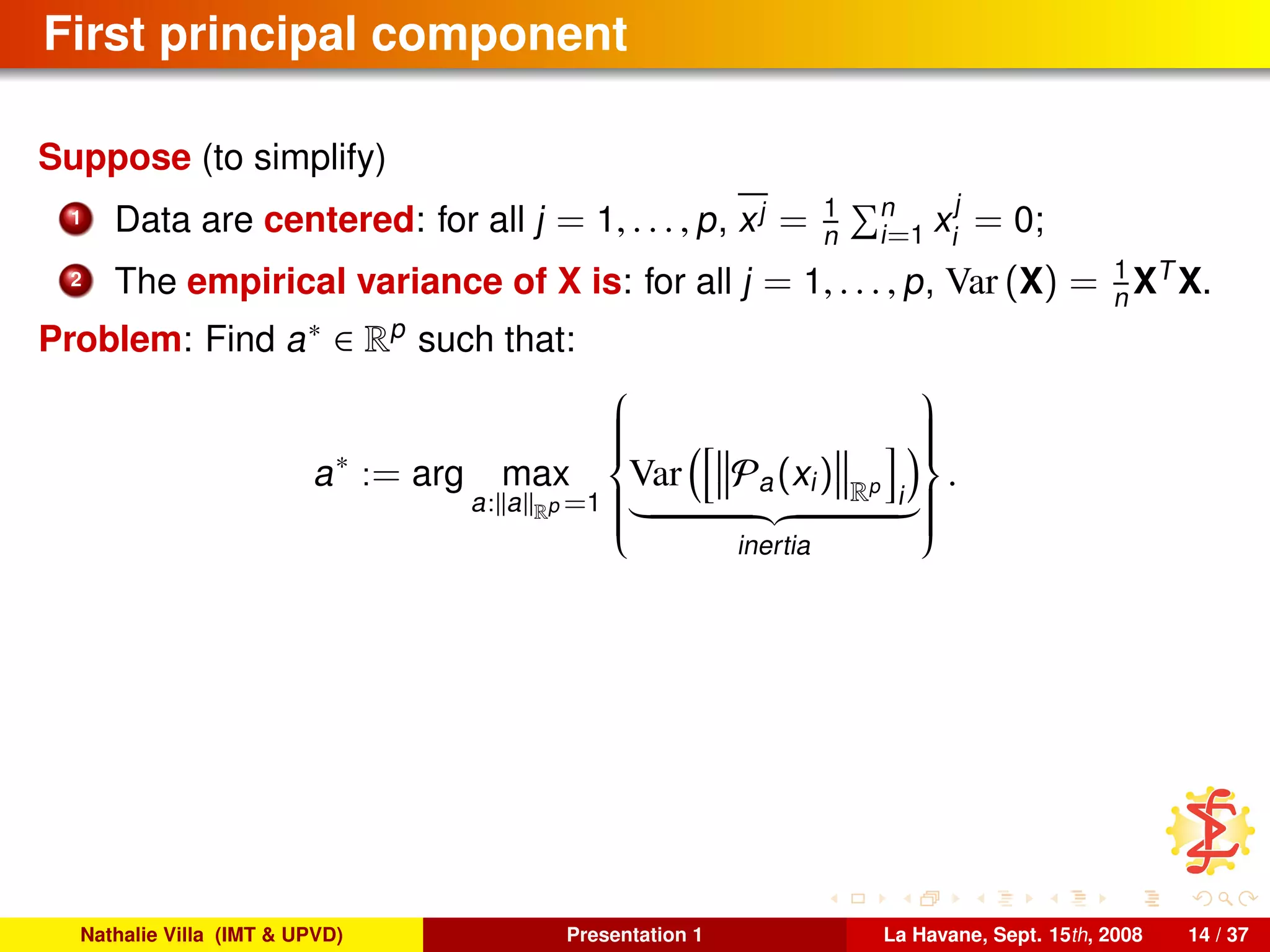
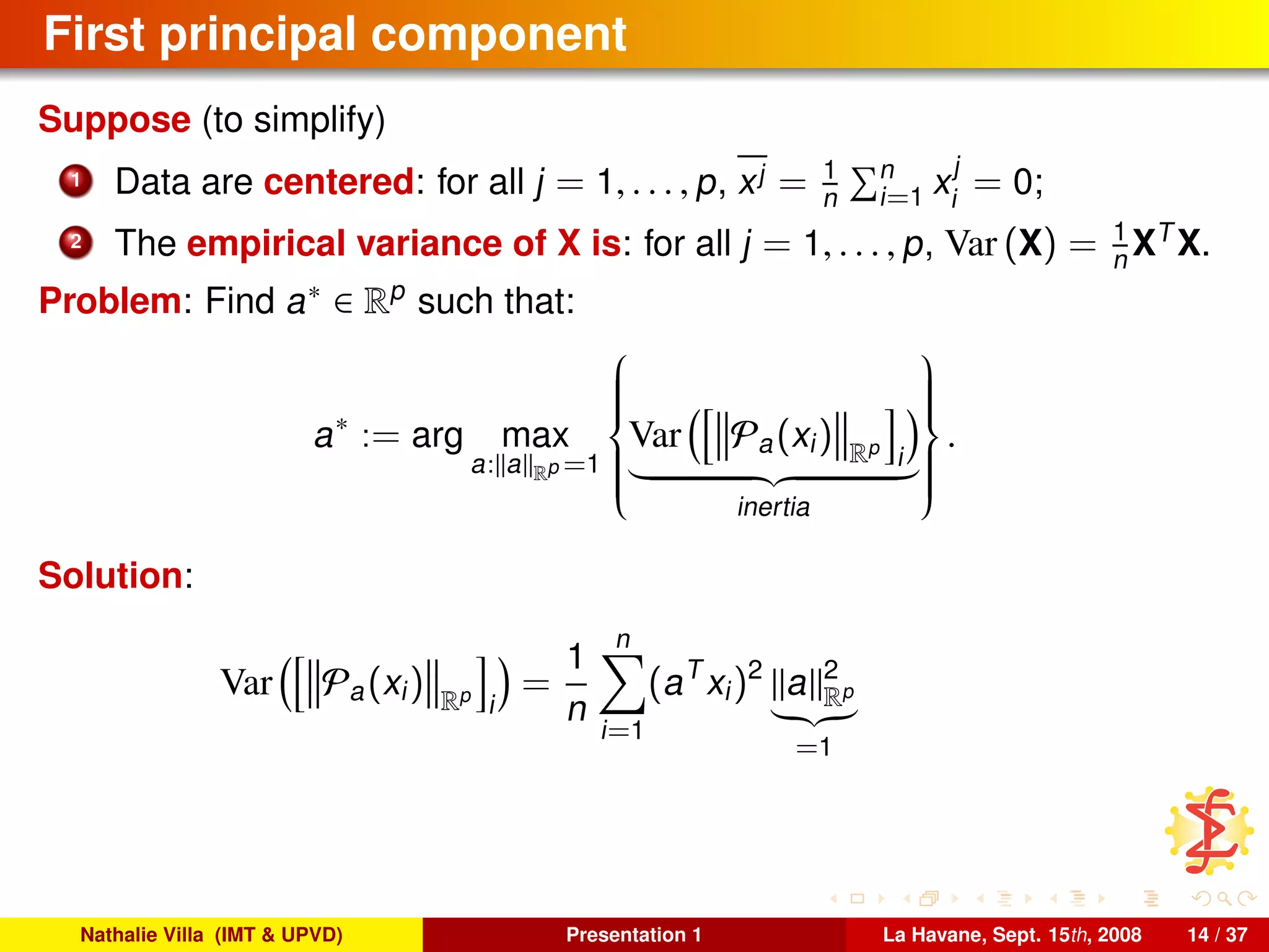
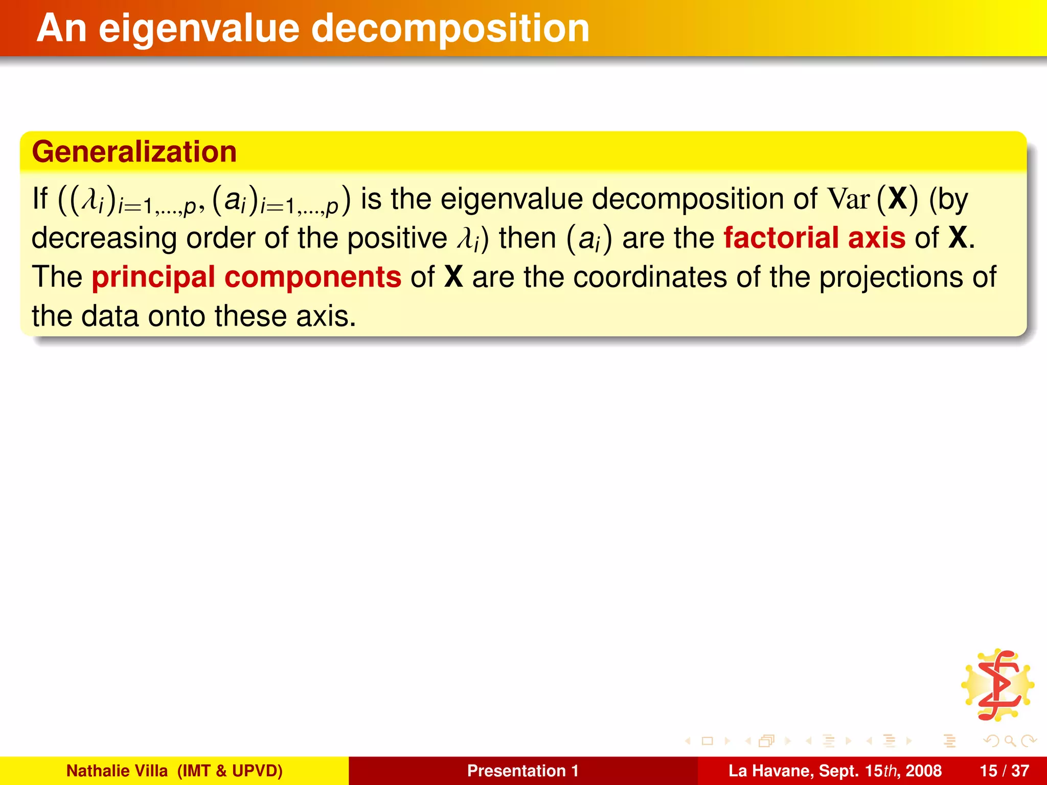
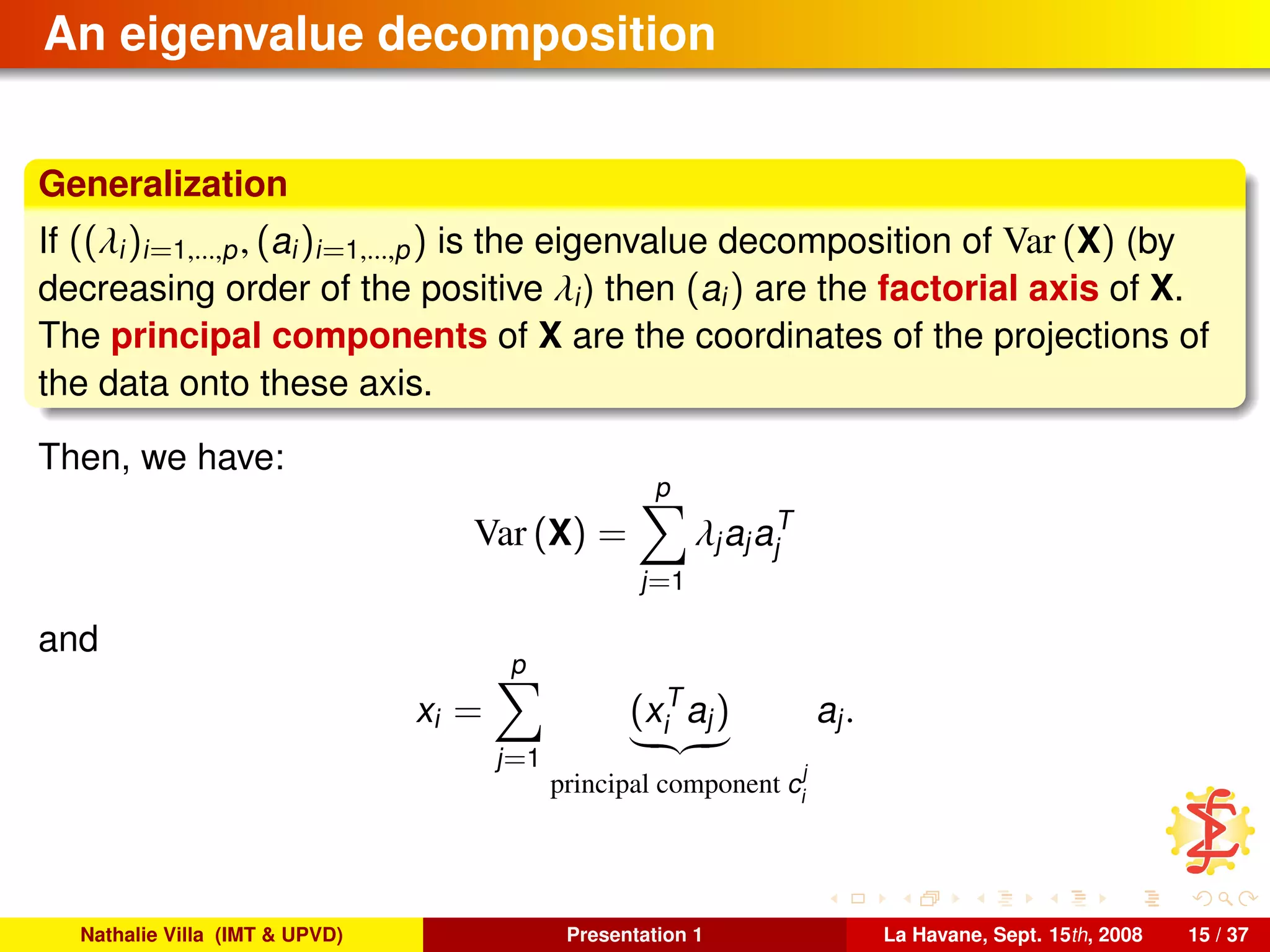
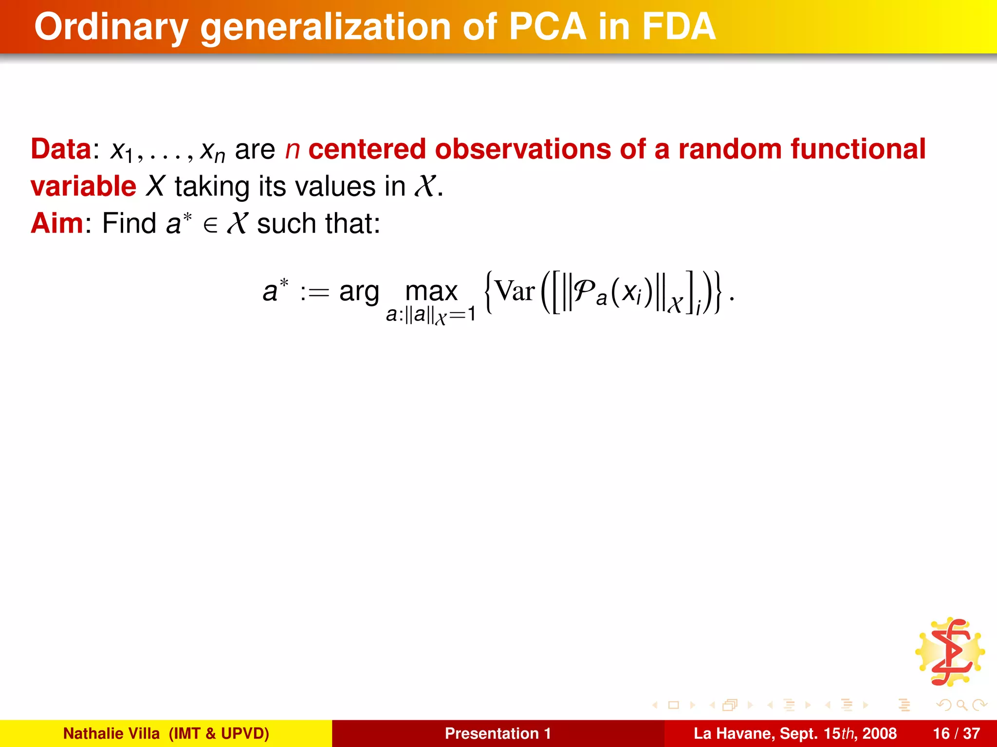
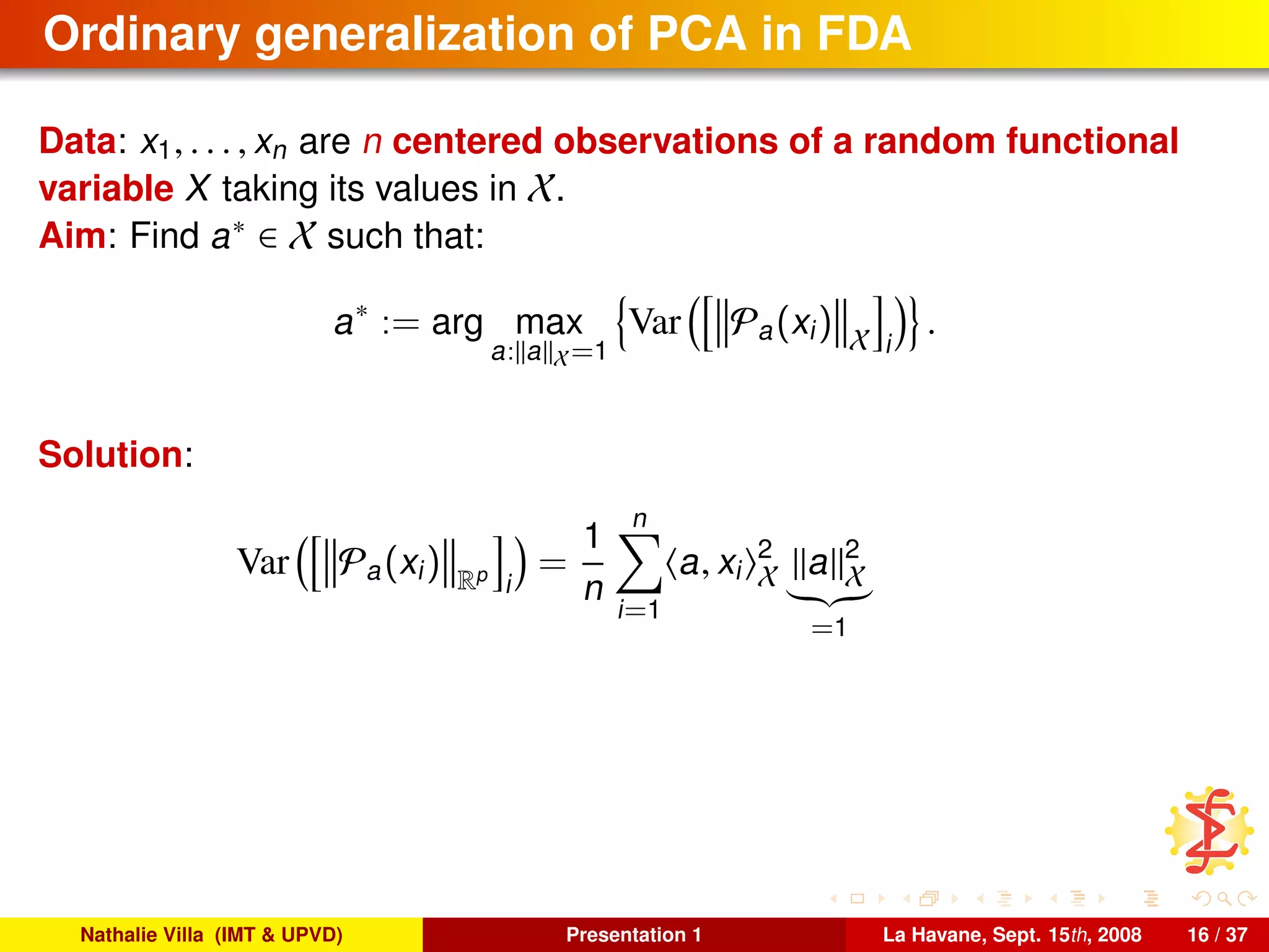
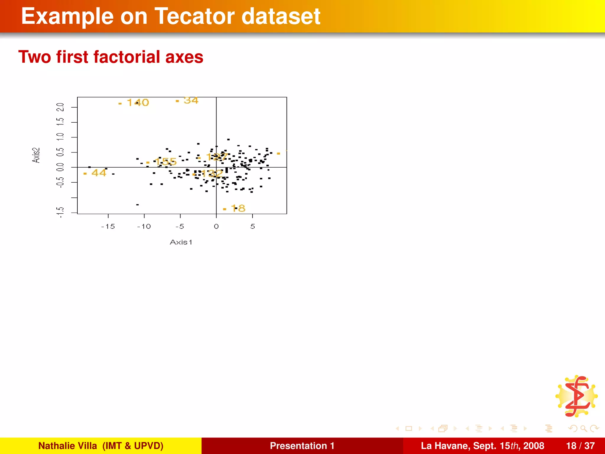
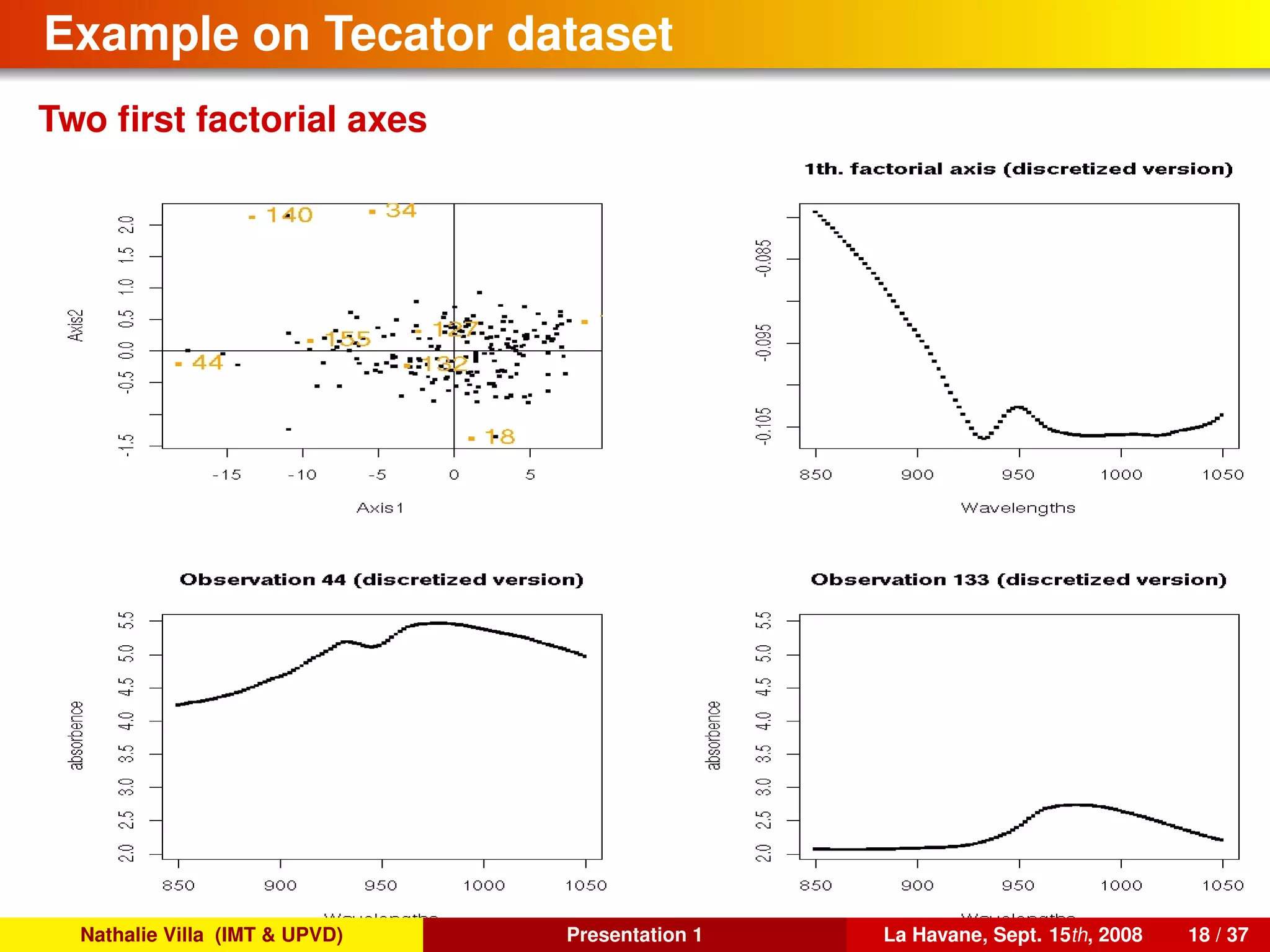
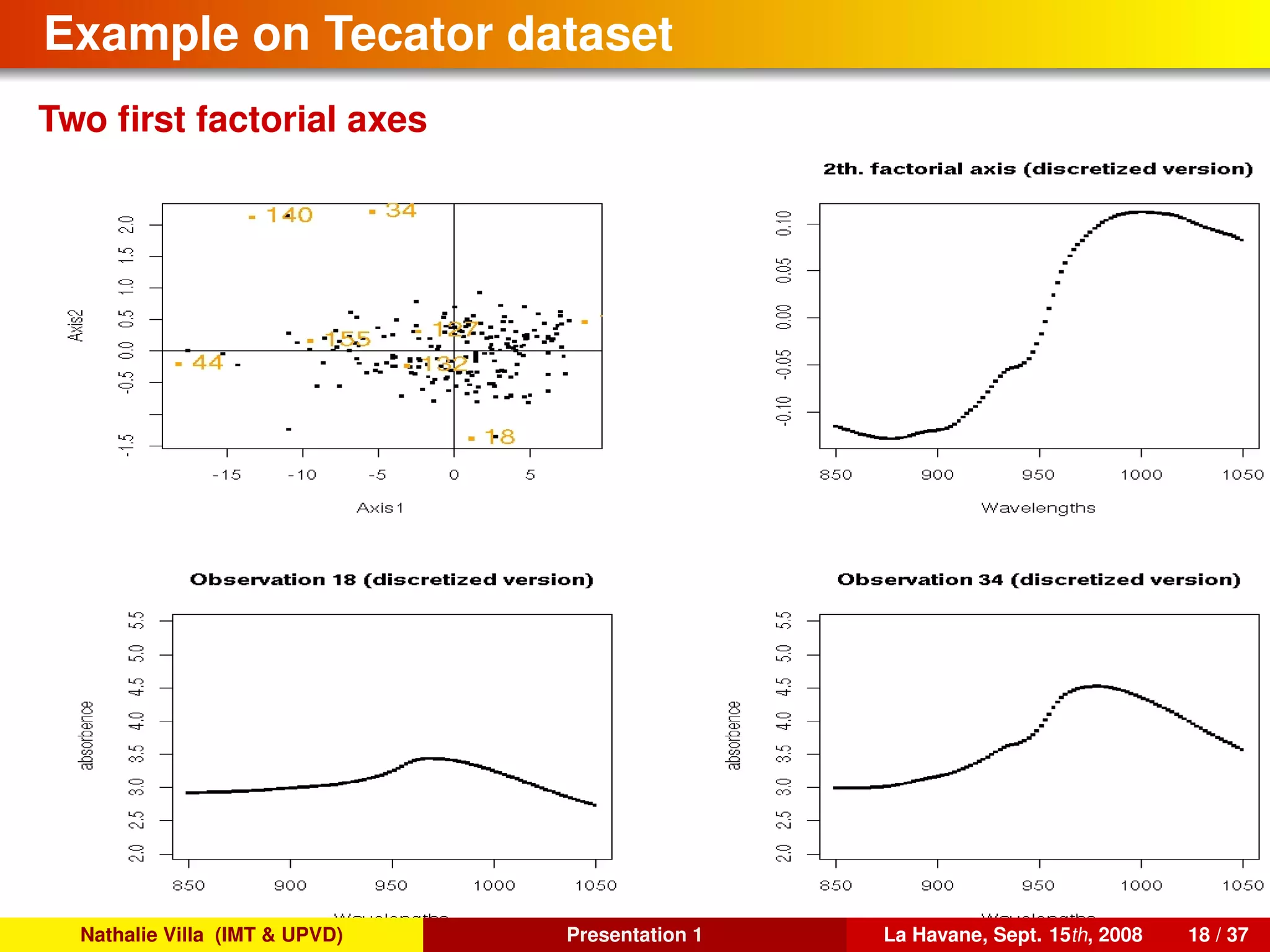
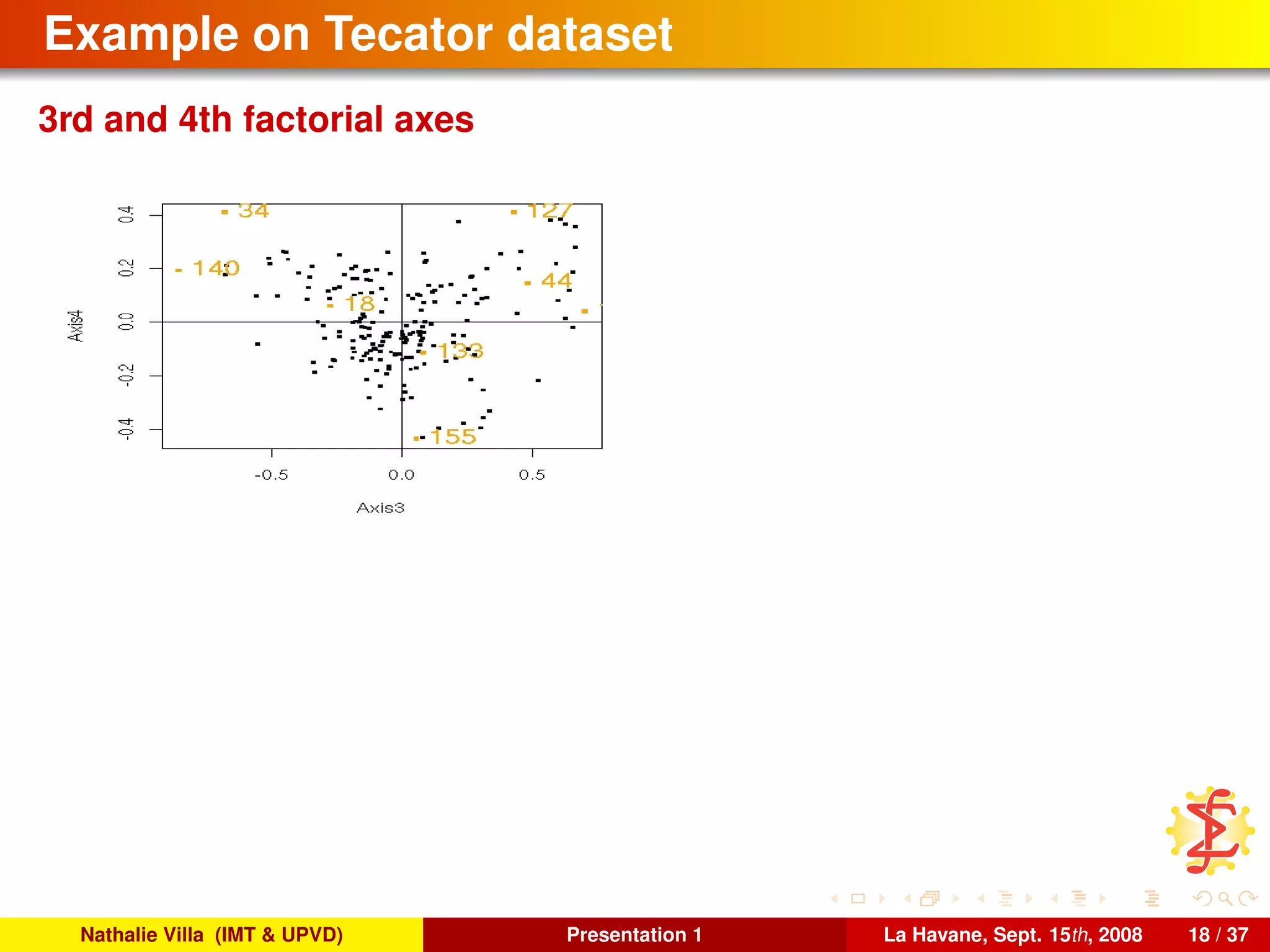
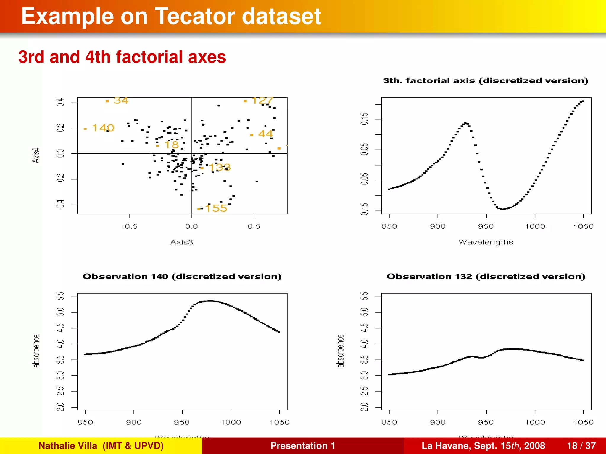
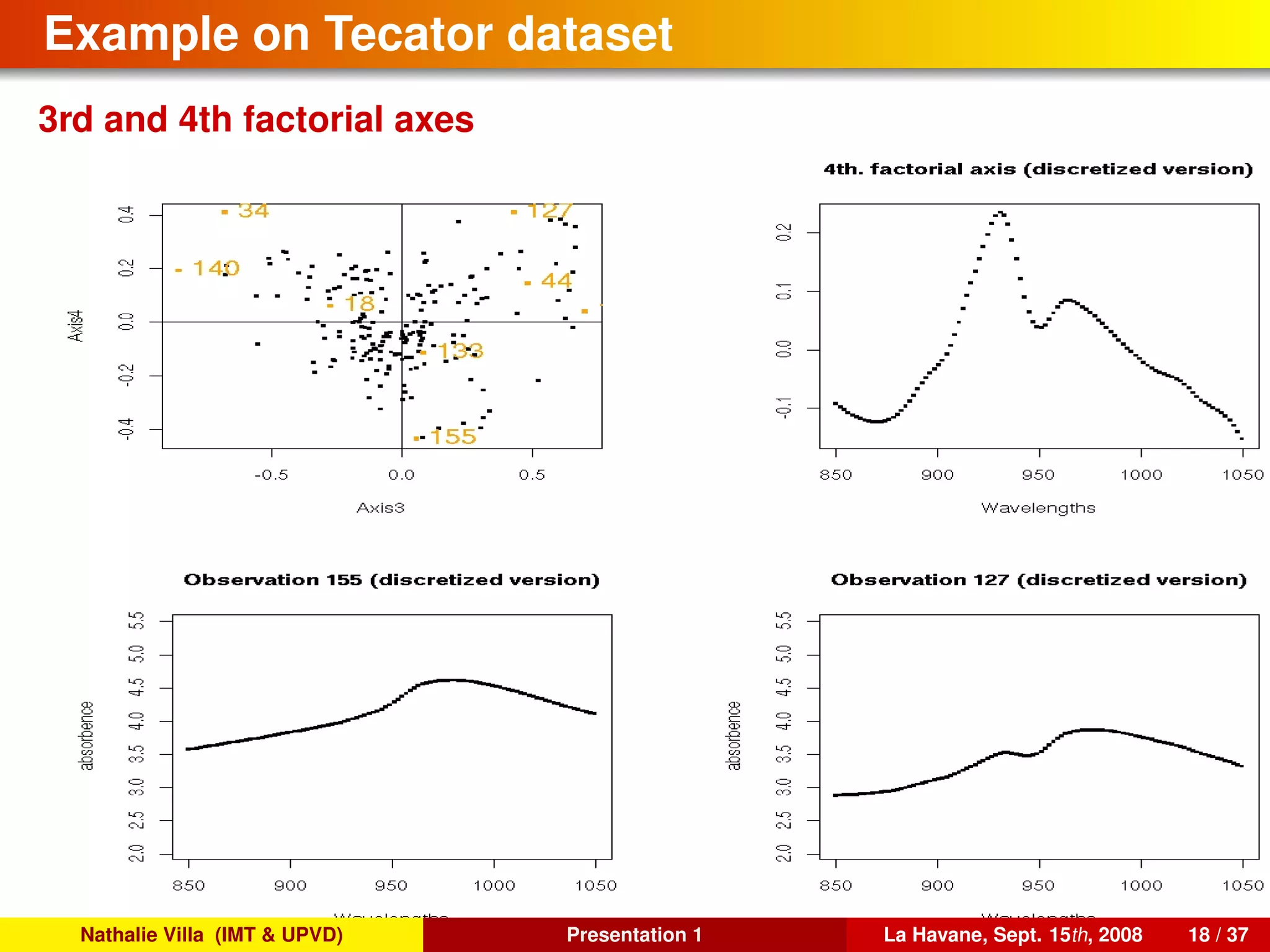
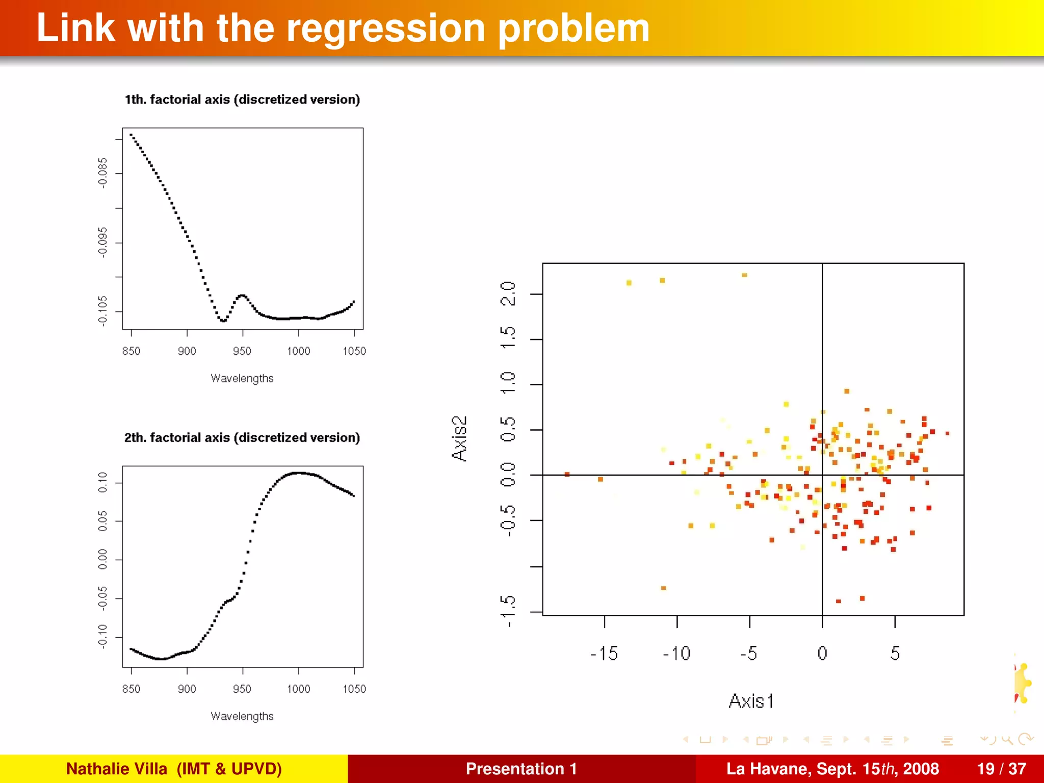
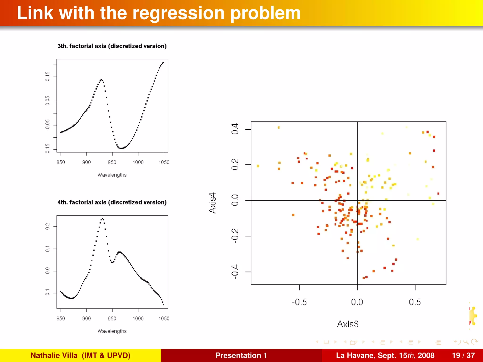
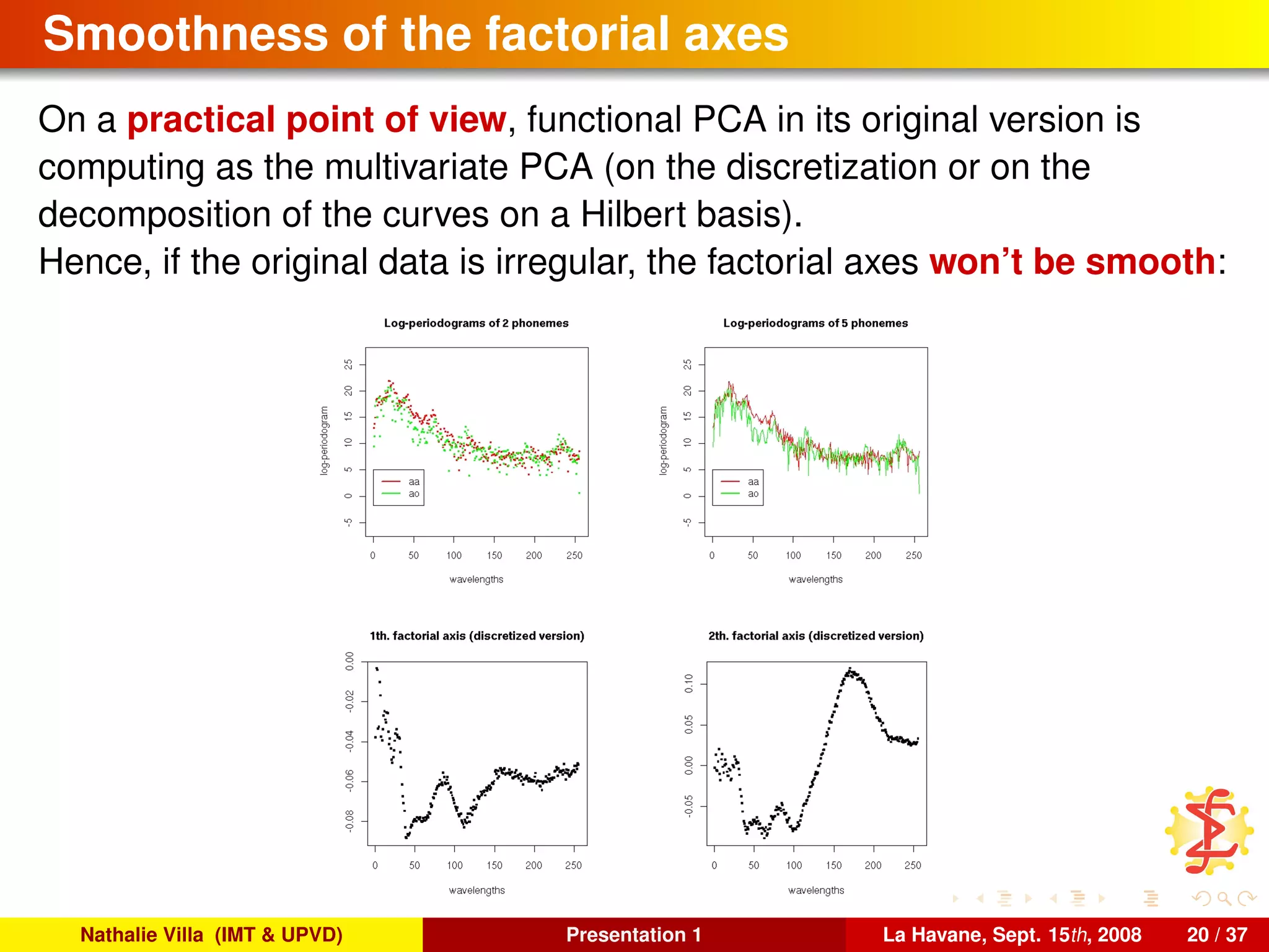
The document provides an introduction to Functional Data Analysis (FDA) and its application in modeling continuous phenomena through linear models. It discusses various examples of FDA, emphasizes the challenges posed by high-dimensional and highly correlated data, and introduces theoretical foundations including functional random variables in Hilbert spaces. The content is geared toward understanding the implications of FDA for statistical methods and modeling complexities.
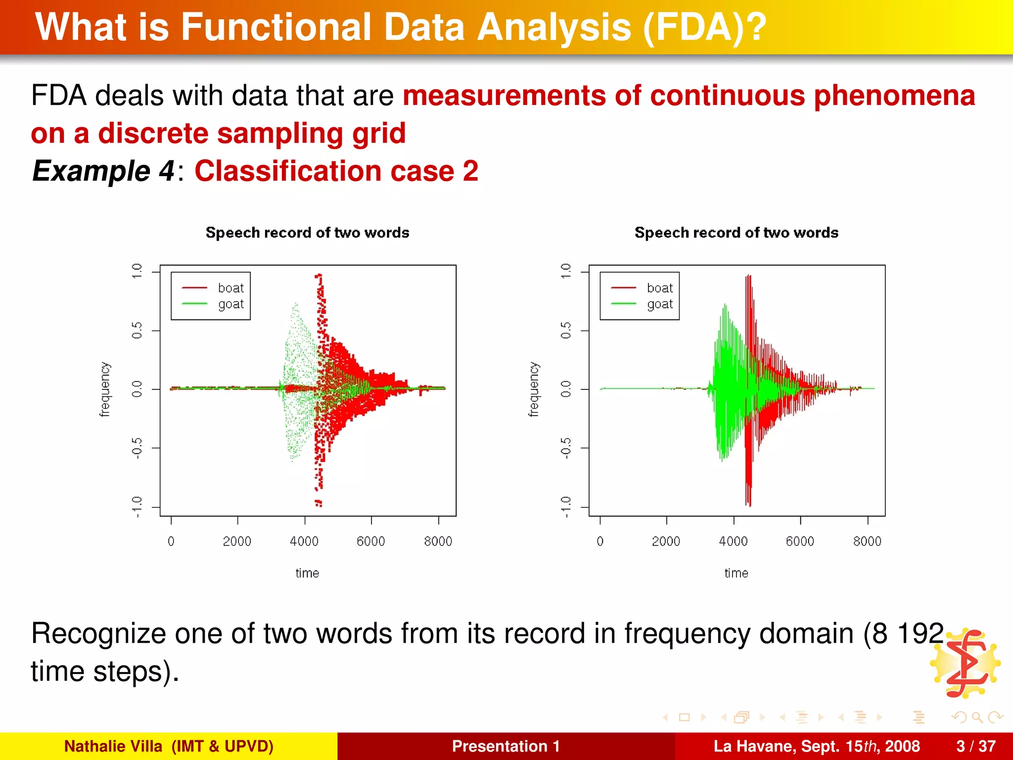
![What is Functional Data Analysis (FDA)?
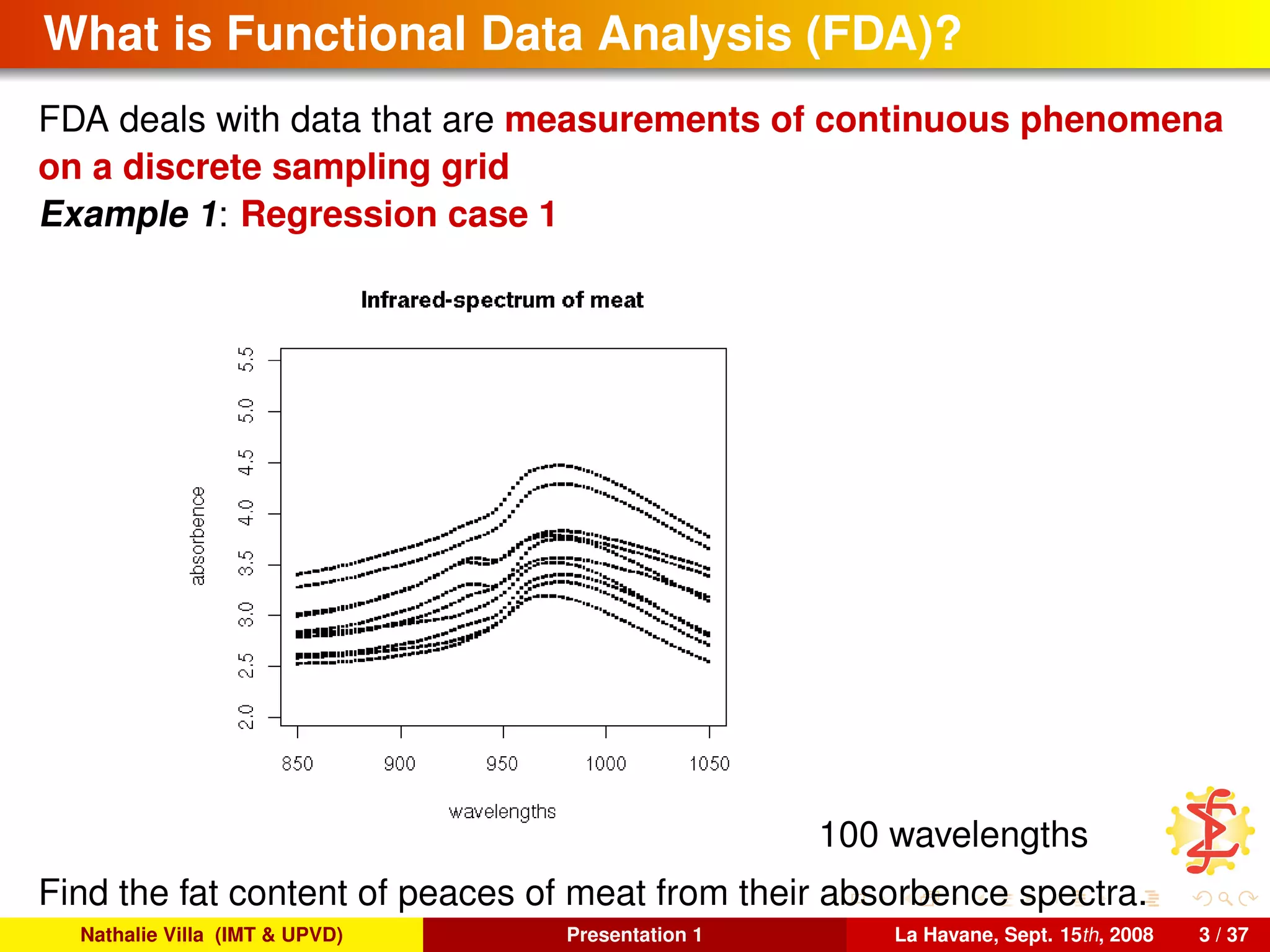
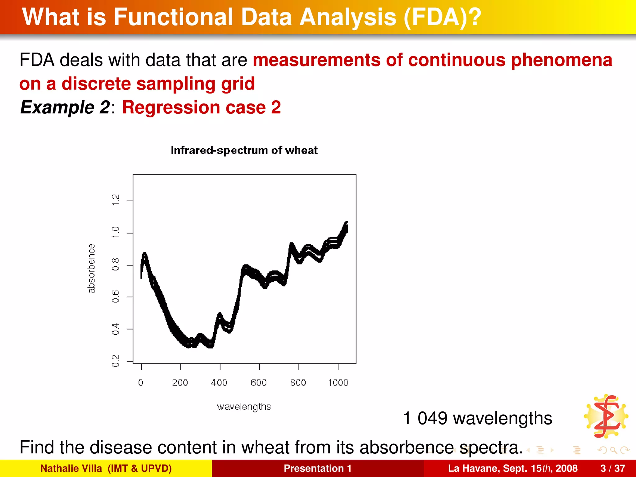
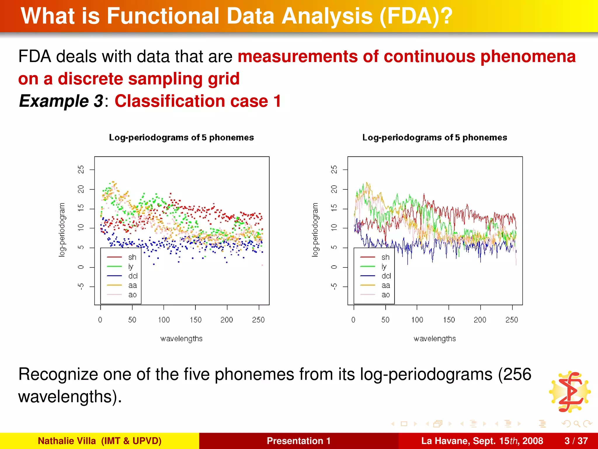
FDA deals with data that are measurements of continuous phenomena
on a discrete sampling grid
Example 5: Regression on functional data
[Azaïs et al., 2008]
Estimate a typical load curve (electricity consumption) from economic
multivariate variables.
Nathalie Villa (IMT & UPVD) Presentation 1 La Havane, Sept. 15th, 2008 3 / 37](https://image.slidesharecdn.com/cenatav2008-09-15-140812085325-phpapp01/75/Introduction-to-FDA-and-linear-models-8-2048.jpg)
![What is Functional Data Analysis (FDA)?
FDA deals with data that are measurements of continuous phenomena
on a discrete sampling grid
Example 6: Curves clustering
[Bensmail et al., 2005]
Create a typology of sick cells from their “SELDI mass” spectra.
Nathalie Villa (IMT & UPVD) Presentation 1 La Havane, Sept. 15th, 2008 3 / 37](https://image.slidesharecdn.com/cenatav2008-09-15-140812085325-phpapp01/75/Introduction-to-FDA-and-linear-models-9-2048.jpg)

![Case X = L2
([0, 1])
if X = L2
([0, 1]), this expressions simplify in:
norm: X 2
= [0,1]
(X(t))2
dt < +∞;
Nathalie Villa (IMT & UPVD) Presentation 1 La Havane, Sept. 15th, 2008 7 / 37](https://image.slidesharecdn.com/cenatav2008-09-15-140812085325-phpapp01/75/Introduction-to-FDA-and-linear-models-19-2048.jpg)
![Case X = L2
([0, 1])
if X = L2
([0, 1]), this expressions simplify in:
norm: X 2
= [0,1]
(X(t))2
dt < +∞;
expectation: for all t ∈ [0, 1],
E (X) (t) = E (X(t)) = X(t)dPX ,
Nathalie Villa (IMT & UPVD) Presentation 1 La Havane, Sept. 15th, 2008 7 / 37](https://image.slidesharecdn.com/cenatav2008-09-15-140812085325-phpapp01/75/Introduction-to-FDA-and-linear-models-20-2048.jpg)
![Case X = L2
([0, 1])
if X = L2
([0, 1]), this expressions simplify in:
norm: X 2
= [0,1]
(X(t))2
dt < +∞;
expectation: for all t ∈ [0, 1],
E (X) (t) = E (X(t)) = X(t)dPX ,
variance: for all t, t ∈ [0, 1],
ΓX γ(t, t ) = E (X(t)X(t ))
(if E (X) = 0 for clarity reasons)
Nathalie Villa (IMT & UPVD) Presentation 1 La Havane, Sept. 15th, 2008 7 / 37](https://image.slidesharecdn.com/cenatav2008-09-15-140812085325-phpapp01/75/Introduction-to-FDA-and-linear-models-21-2048.jpg)
![Case X = L2
([0, 1])
if X = L2
([0, 1]), this expressions simplify in:
norm: X 2
= [0,1]
(X(t))2
dt < +∞;
expectation: for all t ∈ [0, 1],
E (X) (t) = E (X(t)) = X(t)dPX ,
variance: for all t, t ∈ [0, 1],
ΓX γ(t, t ) = E (X(t)X(t ))
(if E (X) = 0 for clarity reasons) because:
1 for all t ∈ [0, 1], we can define Γt
X
: u ∈ X → (ΓX u)(t) ∈ R,
Nathalie Villa (IMT & UPVD) Presentation 1 La Havane, Sept. 15th, 2008 7 / 37](https://image.slidesharecdn.com/cenatav2008-09-15-140812085325-phpapp01/75/Introduction-to-FDA-and-linear-models-22-2048.jpg)
![Case X = L2
([0, 1])
if X = L2
([0, 1]), this expressions simplify in:
norm: X 2
= [0,1]
(X(t))2
dt < +∞;
expectation: for all t ∈ [0, 1],
E (X) (t) = E (X(t)) = X(t)dPX ,
variance: for all t, t ∈ [0, 1],
ΓX γ(t, t ) = E (X(t)X(t ))
(if E (X) = 0 for clarity reasons) because:
1 for all t ∈ [0, 1], we can define Γt
X
: u ∈ X → (ΓX u)(t) ∈ R,
2 By Riesz’s Theorem, it exists ζt
∈ X such that ∀ u ∈ X, Γt
X
u = ζt
, u X.
Nathalie Villa (IMT & UPVD) Presentation 1 La Havane, Sept. 15th, 2008 7 / 37](https://image.slidesharecdn.com/cenatav2008-09-15-140812085325-phpapp01/75/Introduction-to-FDA-and-linear-models-23-2048.jpg)
![Case X = L2
([0, 1])
if X = L2
([0, 1]), this expressions simplify in:
norm: X 2
= [0,1]
(X(t))2
dt < +∞;
expectation: for all t ∈ [0, 1],
E (X) (t) = E (X(t)) = X(t)dPX ,
variance: for all t, t ∈ [0, 1],
ΓX γ(t, t ) = E (X(t)X(t ))
(if E (X) = 0 for clarity reasons) because:
1 for all t ∈ [0, 1], we can define Γt
X
: u ∈ X → (ΓX u)(t) ∈ R,
2 By Riesz’s Theorem, it exists ζt
∈ X such that ∀ u ∈ X, Γt
X
u = ζt
, u X.
As,
(ΓX u)(t) = E ( X, u XX(t))
Nathalie Villa (IMT & UPVD) Presentation 1 La Havane, Sept. 15th, 2008 7 / 37](https://image.slidesharecdn.com/cenatav2008-09-15-140812085325-phpapp01/75/Introduction-to-FDA-and-linear-models-24-2048.jpg)
![Case X = L2
([0, 1])
if X = L2
([0, 1]), this expressions simplify in:
norm: X 2
= [0,1]
(X(t))2
dt < +∞;
expectation: for all t ∈ [0, 1],
E (X) (t) = E (X(t)) = X(t)dPX ,
variance: for all t, t ∈ [0, 1],
ΓX γ(t, t ) = E (X(t)X(t ))
(if E (X) = 0 for clarity reasons) because:
1 for all t ∈ [0, 1], we can define Γt
X
: u ∈ X → (ΓX u)(t) ∈ R,
2 By Riesz’s Theorem, it exists ζt
∈ X such that ∀ u ∈ X, Γt
X
u = ζt
, u X.
As,
(ΓX u)(t) = E ( X(t)X, u X)
Nathalie Villa (IMT & UPVD) Presentation 1 La Havane, Sept. 15th, 2008 7 / 37](https://image.slidesharecdn.com/cenatav2008-09-15-140812085325-phpapp01/75/Introduction-to-FDA-and-linear-models-25-2048.jpg)
![Case X = L2
([0, 1])
if X = L2
([0, 1]), this expressions simplify in:
norm: X 2
= [0,1]
(X(t))2
dt < +∞;
expectation: for all t ∈ [0, 1],
E (X) (t) = E (X(t)) = X(t)dPX ,
variance: for all t, t ∈ [0, 1],
ΓX γ(t, t ) = E (X(t)X(t ))
(if E (X) = 0 for clarity reasons) because:
1 for all t ∈ [0, 1], we can define Γt
X
: u ∈ X → (ΓX u)(t) ∈ R,
2 By Riesz’s Theorem, it exists ζt
∈ X such that ∀ u ∈ X, Γt
X
u = ζt
, u X.
As,
(ΓX u)(t) = E (X(t)X), u X,
Nathalie Villa (IMT & UPVD) Presentation 1 La Havane, Sept. 15th, 2008 7 / 37](https://image.slidesharecdn.com/cenatav2008-09-15-140812085325-phpapp01/75/Introduction-to-FDA-and-linear-models-26-2048.jpg)
![Case X = L2
([0, 1])
if X = L2
([0, 1]), this expressions simplify in:
norm: X 2
= [0,1]
(X(t))2
dt < +∞;
expectation: for all t ∈ [0, 1],
E (X) (t) = E (X(t)) = X(t)dPX ,
variance: for all t, t ∈ [0, 1],
ΓX γ(t, t ) = E (X(t)X(t ))
(if E (X) = 0 for clarity reasons) because:
1 for all t ∈ [0, 1], we can define Γt
X
: u ∈ X → (ΓX u)(t) ∈ R,
2 By Riesz’s Theorem, it exists ζt
∈ X such that ∀ u ∈ X, Γt
X
u = ζt
, u X.
As,
(ΓX u)(t) = E (X(t)X), u X,
we have that ζt
= E (X(t)X) .
Nathalie Villa (IMT & UPVD) Presentation 1 La Havane, Sept. 15th, 2008 7 / 37](https://image.slidesharecdn.com/cenatav2008-09-15-140812085325-phpapp01/75/Introduction-to-FDA-and-linear-models-27-2048.jpg)
![Case X = L2
([0, 1])
if X = L2
([0, 1]), this expressions simplify in:
norm: X 2
= [0,1]
(X(t))2
dt < +∞;
expectation: for all t ∈ [0, 1],
E (X) (t) = E (X(t)) = X(t)dPX ,
variance: for all t, t ∈ [0, 1],
ΓX γ(t, t ) = E (X(t)X(t ))
(if E (X) = 0 for clarity reasons) because:
1 for all t ∈ [0, 1], we can define Γt
X
: u ∈ X → (ΓX u)(t) ∈ R,
2 By Riesz’s Theorem, it exists ζt
∈ X such that ∀ u ∈ X, Γt
X
u = ζt
, u X.
As,
(ΓX u)(t) = E (X(t)X), u X,
we have that ζt
= E (X(t)X) .
3 We define γ : (t, t ) ∈ [0, 1]2
→ ζt
(t ) = E (X(t)X(t ))
Nathalie Villa (IMT & UPVD) Presentation 1 La Havane, Sept. 15th, 2008 7 / 37](https://image.slidesharecdn.com/cenatav2008-09-15-140812085325-phpapp01/75/Introduction-to-FDA-and-linear-models-28-2048.jpg)


![To conclude, several references. . .
Theoretical background for functional PCA:
[Deville, 1974]
[Dauxois and Pousse, 1976]
Smooth PCA:
[Besse and Ramsay, 1986]
[Pezzulli and Silverman, 1993]
[Silverman, 1996]
Several examples and discussion:
[Ramsay and Silverman, 2002]
[Ramsay and Silverman, 1997]
Nathalie Villa (IMT & UPVD) Presentation 1 La Havane, Sept. 15th, 2008 23 / 37](https://image.slidesharecdn.com/cenatav2008-09-15-140812085325-phpapp01/75/Introduction-to-FDA-and-linear-models-93-2048.jpg)
![PCA approach
References: [Cardot et al., 1999] from the works of [Bosq, 1991] on
hilbertian AR models.
Nathalie Villa (IMT & UPVD) Presentation 1 La Havane, Sept. 15th, 2008 27 / 37](https://image.slidesharecdn.com/cenatav2008-09-15-140812085325-phpapp01/75/Introduction-to-FDA-and-linear-models-102-2048.jpg)
![PCA approach
References: [Cardot et al., 1999] from the works of [Bosq, 1991] on
hilbertian AR models.
PCA decomposition of X: Note
((λn
i
, vn
i
))i≥1 the eigenvalue decomposition of Γn
X
((λi)i are ordered in
decreasing order and almost n eigenvalues are not null; (vn
i
)i are
orthonormal)
Nathalie Villa (IMT & UPVD) Presentation 1 La Havane, Sept. 15th, 2008 27 / 37](https://image.slidesharecdn.com/cenatav2008-09-15-140812085325-phpapp01/75/Introduction-to-FDA-and-linear-models-103-2048.jpg)
![PCA approach
References: [Cardot et al., 1999] from the works of [Bosq, 1991] on
hilbertian AR models.
PCA decomposition of X: Note
((λn
i
, vn
i
))i≥1 the eigenvalue decomposition of Γn
X
((λi)i are ordered in
decreasing order and almost n eigenvalues are not null; (vn
i
)i are
orthonormal)
kn an integer such that: kn ≤ n and limn→+∞ kn = +∞
Nathalie Villa (IMT & UPVD) Presentation 1 La Havane, Sept. 15th, 2008 27 / 37](https://image.slidesharecdn.com/cenatav2008-09-15-140812085325-phpapp01/75/Introduction-to-FDA-and-linear-models-104-2048.jpg)
![PCA approach
References: [Cardot et al., 1999] from the works of [Bosq, 1991] on
hilbertian AR models.
PCA decomposition of X: Note
((λn
i
, vn
i
))i≥1 the eigenvalue decomposition of Γn
X
((λi)i are ordered in
decreasing order and almost n eigenvalues are not null; (vn
i
)i are
orthonormal)
kn an integer such that: kn ≤ n and limn→+∞ kn = +∞
Pkn the projector Pkn (u) = kn
i=1
vn
i
, . Xvn
i
Nathalie Villa (IMT & UPVD) Presentation 1 La Havane, Sept. 15th, 2008 27 / 37](https://image.slidesharecdn.com/cenatav2008-09-15-140812085325-phpapp01/75/Introduction-to-FDA-and-linear-models-105-2048.jpg)
![PCA approach
References: [Cardot et al., 1999] from the works of [Bosq, 1991] on
hilbertian AR models.
PCA decomposition of X: Note
((λn
i
, vn
i
))i≥1 the eigenvalue decomposition of Γn
X
((λi)i are ordered in
decreasing order and almost n eigenvalues are not null; (vn
i
)i are
orthonormal)
kn an integer such that: kn ≤ n and limn→+∞ kn = +∞
Pkn the projector Pkn (u) = kn
i=1
vn
i
, . Xvn
i
Γn,kn
X
= Pkn ◦ Γn,kn
X
◦ Pkn = 1
n
kn
i=1
λn
i
vn
i
, . Xvn
i
Nathalie Villa (IMT & UPVD) Presentation 1 La Havane, Sept. 15th, 2008 27 / 37](https://image.slidesharecdn.com/cenatav2008-09-15-140812085325-phpapp01/75/Introduction-to-FDA-and-linear-models-106-2048.jpg)
![PCA approach
References: [Cardot et al., 1999] from the works of [Bosq, 1991] on
hilbertian AR models.
PCA decomposition of X: Note
((λn
i
, vn
i
))i≥1 the eigenvalue decomposition of Γn
X
((λi)i are ordered in
decreasing order and almost n eigenvalues are not null; (vn
i
)i are
orthonormal)
kn an integer such that: kn ≤ n and limn→+∞ kn = +∞
Pkn the projector Pkn (u) = kn
i=1
vn
i
, . Xvn
i
Γn,kn
X
= Pkn ◦ Γn,kn
X
◦ Pkn = 1
n
kn
i=1
λn
i
vn
i
, . Xvn
i
∆n,kn
(X,Y)
= Pkn ◦ 1
n
n
i=1 yixi = 1
n i=1,...,n, i =1,...,kn
yi xi, vn
i Xvn
i
Nathalie Villa (IMT & UPVD) Presentation 1 La Havane, Sept. 15th, 2008 27 / 37](https://image.slidesharecdn.com/cenatav2008-09-15-140812085325-phpapp01/75/Introduction-to-FDA-and-linear-models-107-2048.jpg)
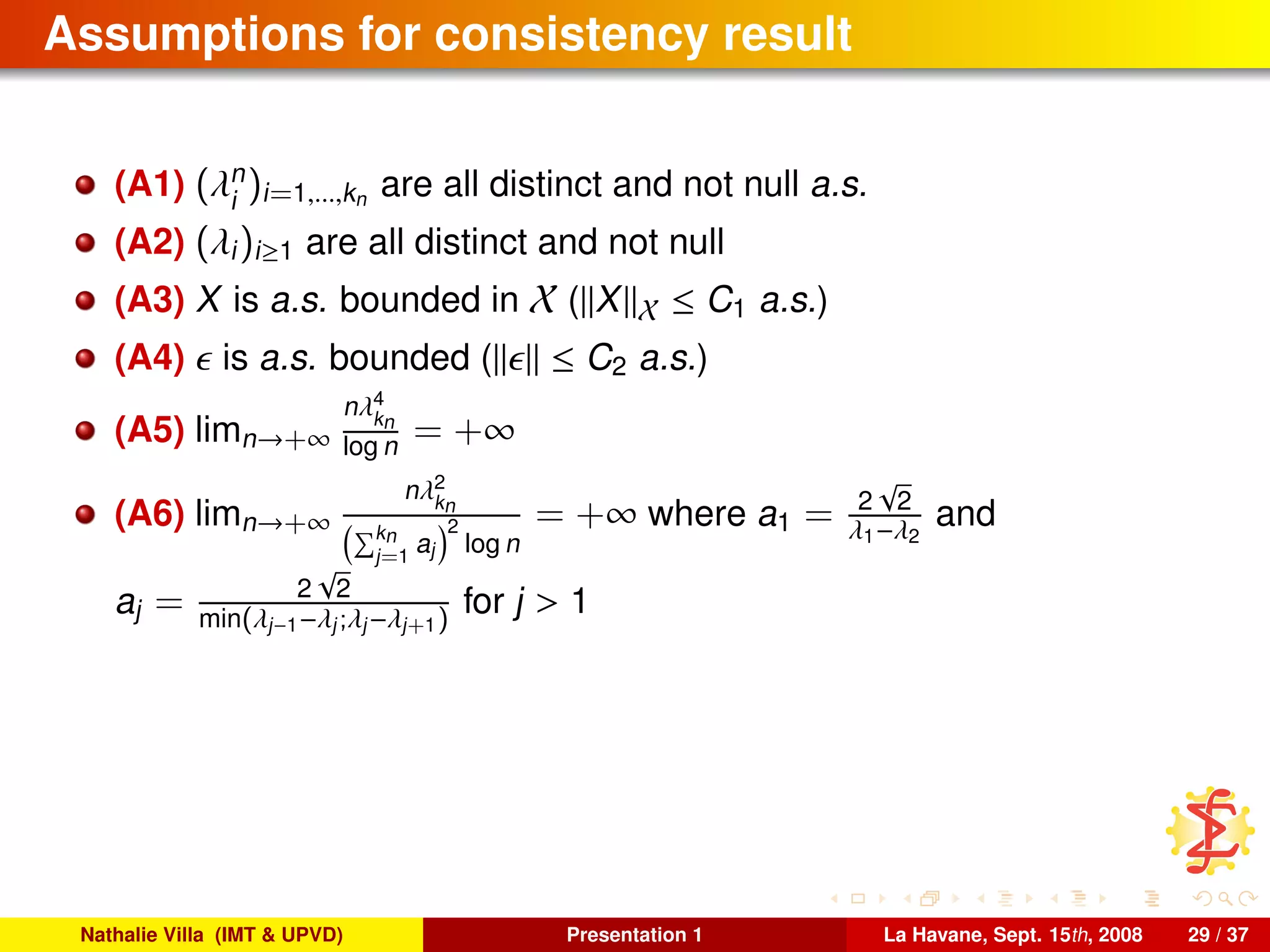
![Assumptions for consistency result
(A1) (λn
i
)i=1,...,kn are all distinct and not null a.s.
(A2) (λi)i≥1 are all distinct and not null
(A3) X is a.s. bounded in X ( X X ≤ C1 a.s.)
(A4) is a.s. bounded ( ≤ C2 a.s.)
(A5) limn→+∞
nλ4
kn
log n = +∞
(A6) limn→+∞
nλ2
kn
kn
j=1
aj
2
log n
= +∞ where a1 = 2
√
2
λ1−λ2
and
aj = 2
√
2
min(λj−1−λj;λj−λj+1)
for j > 1
Example of ΓX satisfying those assumptions: if the eigenvalues of ΓX
are geometrically or exponentially decreasing, these assumptions are
fullfilled as long as the sequence (kn)n tends slowly enough to +∞.
For example, X is a Brownian motion on [0, 1] and kn = o(log n).
Nathalie Villa (IMT & UPVD) Presentation 1 La Havane, Sept. 15th, 2008 29 / 37](https://image.slidesharecdn.com/cenatav2008-09-15-140812085325-phpapp01/75/Introduction-to-FDA-and-linear-models-110-2048.jpg)
![Consistency result
Theorem [Cardot et al., 1999]
Under assumptions (A1)-(A6), we have:
αn
− α X
n→+∞
−−−−−−→ 0
Nathalie Villa (IMT & UPVD) Presentation 1 La Havane, Sept. 15th, 2008 30 / 37](https://image.slidesharecdn.com/cenatav2008-09-15-140812085325-phpapp01/75/Introduction-to-FDA-and-linear-models-111-2048.jpg)
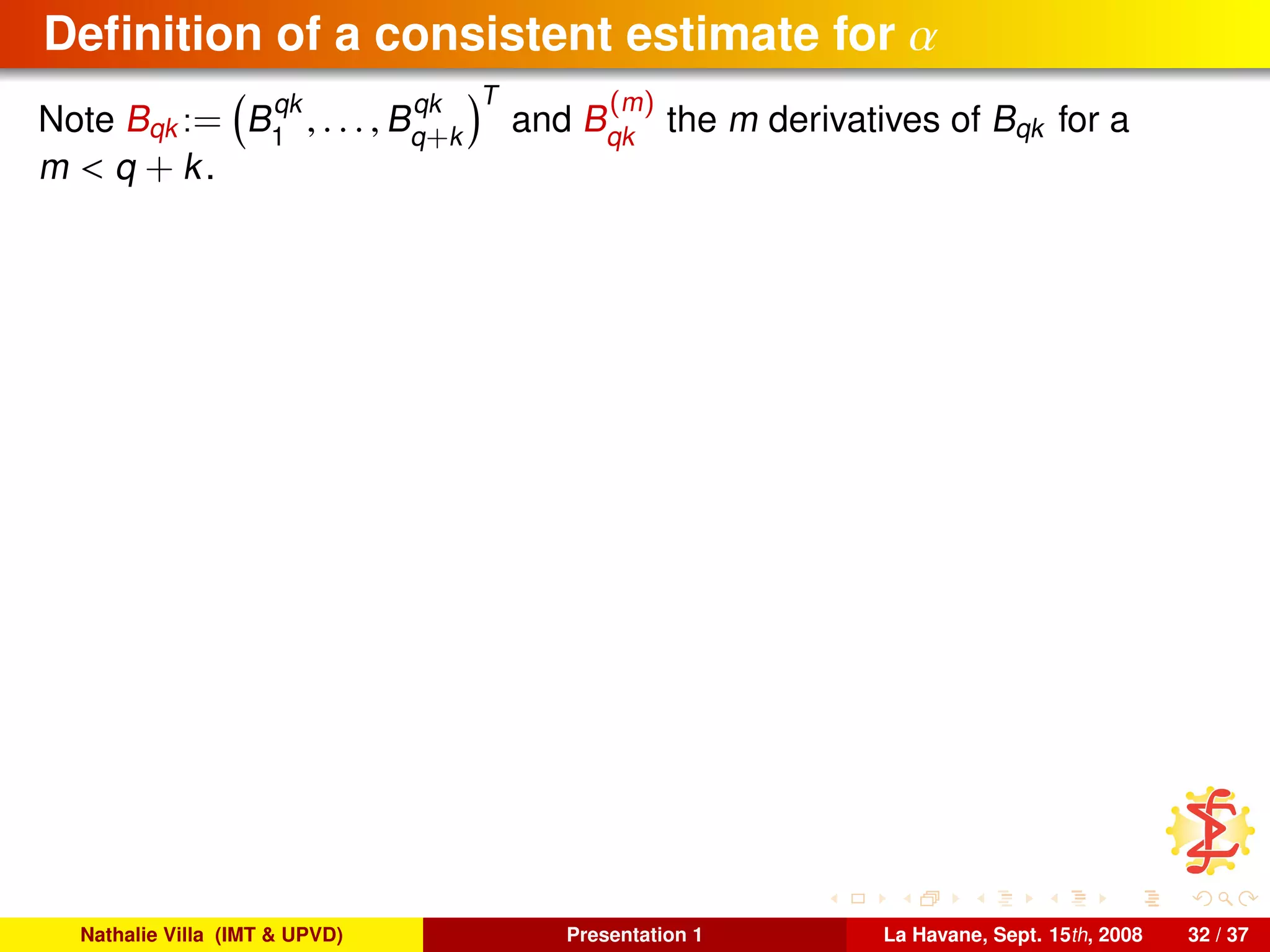
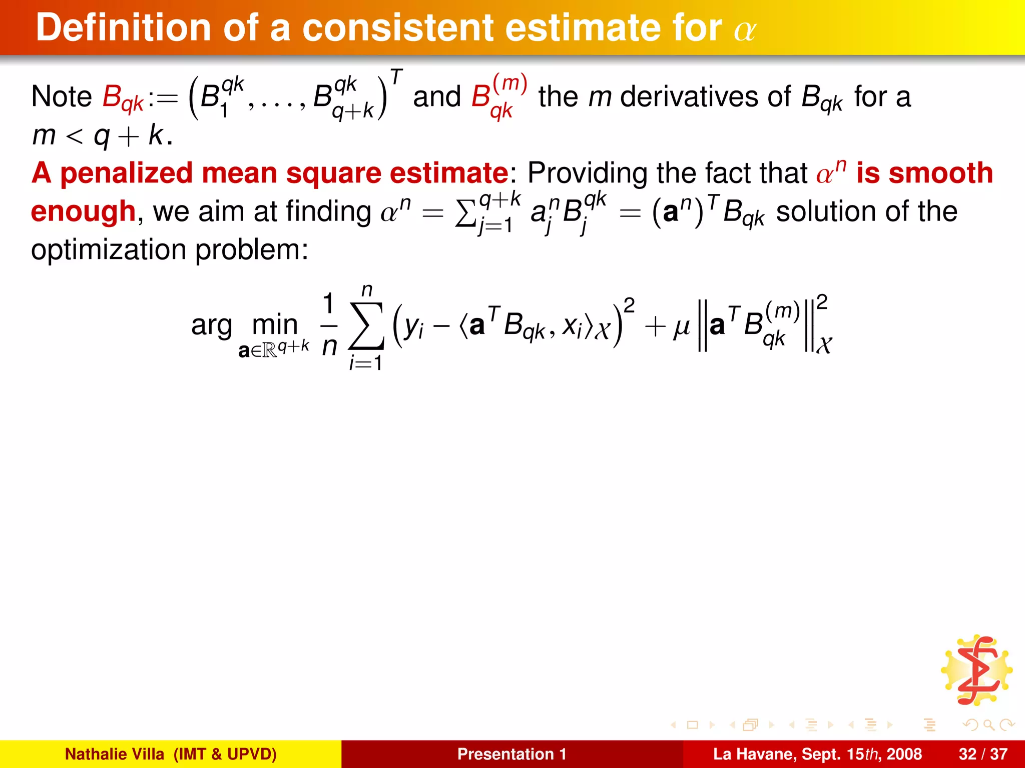
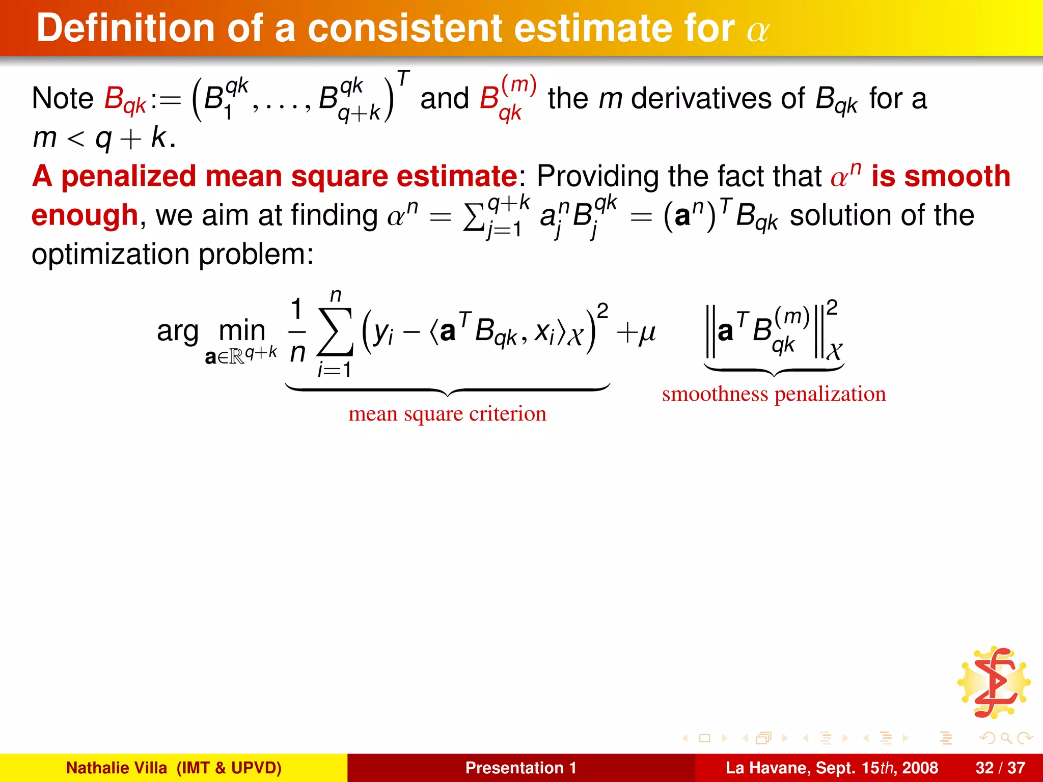
![Smoothing approach based on B-splines
References: [Cardot et al., 2003]
Nathalie Villa (IMT & UPVD) Presentation 1 La Havane, Sept. 15th, 2008 31 / 37](https://image.slidesharecdn.com/cenatav2008-09-15-140812085325-phpapp01/75/Introduction-to-FDA-and-linear-models-112-2048.jpg)
![Smoothing approach based on B-splines
References: [Cardot et al., 2003]
Suppose that X takes values in L2
([0, 1]).
Basics on B-splines: Let q and k be to integers and denotes by Sqk the
space of functions satisfying:
s ∈ Sqk are polynomials of degree q on each interval l−1
k , l
k for all
l = 1, . . . , k,
s ∈ Sqk are q − 1 times differentiable on [0, 1].
Nathalie Villa (IMT & UPVD) Presentation 1 La Havane, Sept. 15th, 2008 31 / 37](https://image.slidesharecdn.com/cenatav2008-09-15-140812085325-phpapp01/75/Introduction-to-FDA-and-linear-models-113-2048.jpg)
![Smoothing approach based on B-splines
References: [Cardot et al., 2003]
Suppose that X takes values in L2
([0, 1]).
Basics on B-splines: Let q and k be to integers and denotes by Sqk the
space of functions satisfying:
s ∈ Sqk are polynomials of degree q on each interval l−1
k , l
k for all
l = 1, . . . , k,
s ∈ Sqk are q − 1 times differentiable on [0, 1].
The space Sqk has dimension q + k and a normalized basis of Sqk is
denoted by {B
qk
j
, j = 1, . . . , q + k} (normalized B-Splines, see
[de Boor, 1978]).
Nathalie Villa (IMT & UPVD) Presentation 1 La Havane, Sept. 15th, 2008 31 / 37](https://image.slidesharecdn.com/cenatav2008-09-15-140812085325-phpapp01/75/Introduction-to-FDA-and-linear-models-114-2048.jpg)
![Smoothing approach based on B-splines
References: [Cardot et al., 2003]
Suppose that X takes values in L2
([0, 1]).
Basics on B-splines: Let q and k be to integers and denotes by Sqk the
space of functions satisfying:
s ∈ Sqk are polynomials of degree q on each interval l−1
k , l
k for all
l = 1, . . . , k,
s ∈ Sqk are q − 1 times differentiable on [0, 1].
The space Sqk has dimension q + k and a normalized basis of Sqk is
denoted by {B
qk
j
, j = 1, . . . , q + k} (normalized B-Splines, see
[de Boor, 1978]).
These functions are easy to manipulate and have interesting smoothness
properties. They can be used to express either X and the parameter α as
well as to impose smoothness constrains on α.
Nathalie Villa (IMT & UPVD) Presentation 1 La Havane, Sept. 15th, 2008 31 / 37](https://image.slidesharecdn.com/cenatav2008-09-15-140812085325-phpapp01/75/Introduction-to-FDA-and-linear-models-115-2048.jpg)
![Assumptions for consistency result
(A1) X is a.s. bounded in X
(A2) Var (Y|X = x) ≤ C1 for all x ∈ X
(A3) E (Y|X = x) ≤ C2 for all x ∈ X
(A4) it exists an integer p and a real ν ∈ [0, 1] such that p + ν ≤ q
and α(p )(t1) − α(p )(t2) ≤ |t1 − t2|ν
(A5) µ = O n−(1−δ)/2
for a 0 < δ < 1
(A6) limn→+∞ µk2(m−p) = 0 for p = p + ν
(A7) k = O n1/(4p+1)
Nathalie Villa (IMT & UPVD) Presentation 1 La Havane, Sept. 15th, 2008 33 / 37](https://image.slidesharecdn.com/cenatav2008-09-15-140812085325-phpapp01/75/Introduction-to-FDA-and-linear-models-120-2048.jpg)
![Consistency result
Theorem [Cardot et al., 2003]
Under assumptions (A1)-(A7),
limn→+∞ P (it exists a unique solution to the minimization problem) = 1
E αn
− α 2
X |x1, . . . , xn = OP n−2p/(4p+1)
Nathalie Villa (IMT & UPVD) Presentation 1 La Havane, Sept. 15th, 2008 34 / 37](https://image.slidesharecdn.com/cenatav2008-09-15-140812085325-phpapp01/75/Introduction-to-FDA-and-linear-models-121-2048.jpg)
![Other functional linear methods
Canonical correlation: [Leurgans et al., 1993]
Factorial Discriminant Analysis: [Hastie et al., 1995]
Partial Least Squares: [Preda and Saporta, 2005]
. . .
Nathalie Villa (IMT & UPVD) Presentation 1 La Havane, Sept. 15th, 2008 35 / 37](https://image.slidesharecdn.com/cenatav2008-09-15-140812085325-phpapp01/75/Introduction-to-FDA-and-linear-models-122-2048.jpg)