DOW JONES INDUSTRIAL AVERAGE Time series Data Analysis: Analysis and Results of Data

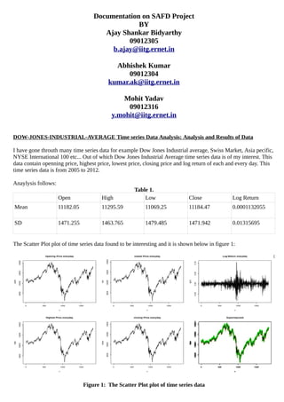
1. Documentation on SAFD Project
BY
Ajay Shankar Bidyarthy
09012305
b.ajay@iitg.ernet.in
Abhishek Kumar
09012304
kumar.ak@iitg.ernet.in
Mohit Yadav
09012316
y.mohit@iitg.ernet.in
DOW-JONES-INDUSTRIAL-AVERAGE Time series Data Analysis: Analysis and Results of Data
I have gone throuth many time series data for example Dow Jones Industrial average, Swiss Market, Asia pecific,
NYSE International 100 etc... Out of which Dow Jones Industrial Average time series data is of my interest. This
data contain openning price, highest price, lowest price, closing price and log return of each and every day. This
time series data is from 2005 to 2012.
Anaylysis follows:
Table 1.
Open High Low Close Log Return
Mean 11182.05 11295.59 11069.25 11184.47 0.0001132055
SD 1471.255 1463.765 1479.485 1471.942 0.01315695
The Scatter Plot plot of time series data found to be interesting and it is shown below in figure 1:
Figure 1: The Scatter Plot plot of time series data

2. The superimposed scatterplot of openning price, highest price, lowest price and closing price is shown below in
figure 2:
Figure 2: The superimposed scatterplot of openning price, highest price, lowest price and closing price
The Histogram plot of openning price, highest price, lowest price and closing price, and the superimposed graph
of log Return and normal plot is shown below in figure 3:
figure 3: The Histogram plot of openning price, highest price, lowest price and closing price, and the
superimposed graph of log Return and normal plot
Next graph figure 4. shows Autocorrelation function plot of log-return data of type correlation, covariance, and
partial.

3. Figure 4: Autocorrelation function plot of log-return data of type correlation, covariance, and partial
Next figure 5: represents AR plot of log-return data for method yule-walker, burg, ols, mle and yw:
Figure 5: Plot represents AR plot of log-return data for method yule-walker, burg, ols, mle and yw
Next graph figure 6. shows whether the log-return data is stationary or not. Out of two plot one is Default method
roots of the corresponding AR polynomial and another is Burg method roots of the corresponding AR
polynomial. Its is found that all roots of AR polynomial lies inside an unit circle.

4. Figure 6: shows whether the log-return data is stationary or not
Next plot figure 7. shows the plot of AR(1): Autoregression model of log-return data: Stationary Time series
Model.
First two plot shows autocorrelation plot of two different lags of AR(1) model. Next two plot shows simple
autocorrelation plot and partial aoutocorrelation plot of AR(1) model. Next two plot shows the AR(1) plot of this
model with two different method yule-walker and burg method.
Figure 7: shows the plot of AR(1): Autoregression model of log-return data: Stationary Time series Model
Next plot figure 8. shows the plot of AR(2): Autoregression model of log-return data: Stationary Time series
Model.

5. First two plot shows autocorrelation plot of two different lags of AR(2) model. Next two plot shows simple
autocorrelation plot and partial aoutocorrelation plot of AR(2) model. Next two plot shows the AR(2) plot of this
model with two different method yule-walker and burg method.
Figure 8: shows the plot of AR(2): Autoregression model of log-return data: Stationary Time series Model.
Next job is to verify whether the AR(1) and AR(2) model is stationary or non stationary. In figure 9. We have
plotted the roots of the polynomial along whith an unit circle and verified that whether the roots lies inside the
circle. We have observed that the roots of the polynomial AR(1) and AR(2) is lies in side the unit circle, hnce it
proved that the AR(1) and AR(2) model is stationary.
Figure 9: We have plotted the roots of the polynomial along whith an unit circle and verified that whether

6. the roots lies inside the circle
Next job is to find out the mean and stndard deviation of AR(1) and AR(2) model generated from log-return data.
We have found the following result in table 2.:
Table 2.
AR(1) AR(2)
mean 0.0002792318 0.0001425631
sd 0.01492827 0.01307018
The results shows that mean of AR(1) and AR(2) model is close to zero.
Next job is to find out bootstrap-t confidence intervals of log-return data. Next two table shows the bootstrap-t
confidence limits of log-return model with different confidence levels.
This table 3. shows the Bootstrap-t Confidence Limits estimated confidence points for the mean using variance-
stabilization bootstrap-T method.
Table 3.
Bootstrap-t Confidence level estimated confidence points for the
mean using variance-stabilization
bootstrap-T method
estimated confidence points for the
mean using standard formula for
stand dev of mean rather than an
inner bootstrap loop
0.001 -0.0007307233 -0.0005634083
0.01 -0.0005819501 -0.0004822881
0.025 -0.0004977744 -0.0003602349
0.05 -0.0004150469 -0.0003287742
0.1 -0.0002846829 -0.0002336607
0.5 0.0001071803 0.0001275114
0.9 0.000536211 0.000528693
0.95 0.0006585565 0.0006526679
0.975 0.0007794517 0.0007909542
0.99 0.0008495297 0.0008132326
0.999 0.0008720842 0.0008996211
Next plots, figure 10. is the plot of bootstrap-t confidence interval of log-return data i.e quantile plot of
bootstrap-t method along with normal abline, which shows that how much the is similar to standard normal
distribution:
Figure 10: plot of bootstrap-t confidence interval of log-return data i.e quantile plot of bootstrap-t method

7. along with normal abline
Next job is to find out bootstrap-t confidence intervals of AR(1) model data. Next two table, table 4 and table 5
shows the bootstrap-t confidence limits of AR(1) model with different confidence levels.
This table 4. shows the Bootstrap-t Confidence Limits estimated confidence points for the mean using variance-
stabilization bootstrap-T method.
Table 4.
Bootstrap-t Confidence level estimated confidence points for the
mean using variance-stabilization
bootstrap-T method AR(1) Model
estimated confidence points for the
mean using standard formula for
stand dev of mean rather than an
inner bootstrap loop AR(1) Model
0.001 -0.0008706475 -0.0007929847
0.01 -0.0006634627 -0.0005364274
0.025 -0.0004847622 -0.0002949158
0.05 -0.000344636 -0.0002096313
0.1 -0.0001901081 -0.0001498637
0.5 0.0002680792 0.0002938364
0.9 0.0007174549 0.0007416045
0.95 0.0008298517 0.0008342107
0.975 0.0009238767 0.000893108
0.99 0.0009425914 0.0009708158
0.999 0.0009946744 0.001464537
This table 5. shows the Bootstrap-t Confidence Limits estimated confidence points for the standard deviation
using variance-stabilization bootstrap-T method.
Table 5.
Bootstrap-t Confidence level estimated confidence points for the
standard deviation using variance-
stabilization bootstrap-T method
estimated confidence points for the
standard deviation using standard
formula for stand dev of mean rather
than an inner bootstrap loop
0.001 0.01350699 0.01365689
0.01 0.01380652 0.01398131
0.025 0.01409778 0.01404494
0.05 0.01413915 0.01421174
0.1 0.01430467 0.0143503
0.5 0.01487313 0.01495102
0.9 0.01563718 0.01565043
0.95 0.01587061 0.0158341
0.975 0.01591511 0.01605114
0.99 0.01613755 0.01619159
0.999 0.01616807 0.01632221
Next plots, figure 11. is the plot of bootstrap-t confidence interval of AR(1) Model i.e quantile plot of bootstrap-t
method along with normal abline, which shows that how much the is similar to standard normal distribution:

8. Figure 11: plot of bootstrap-t confidence interval of AR(1) Model i.e quantile plot of bootstrap-t method
along with normal abline
Next job is to find out bootstrap-t confidence intervals of AR(2) model data. Next two table, table 6. and table 7.
shows the bootstrap-t confidence limits of AR(2) model with different confidence levels.
This table 6. shows the Bootstrap-t Confidence Limits estimated confidence points for the mean using variance-
stabilization bootstrap-T method.
Table 6.
Bootstrap-t Confidence level estimated confidence points for the
mean using variance-stabilization
bootstrap-T method AR(2) Model
estimated confidence points for the
mean using standard formula for
stand dev of mean rather than an
inner bootstrap loop AR(2) Model
0.001 -0.0008389193 -0.0006113395
0.01 -0.0005660646 -0.0004777913
0.025 -0.0004538679 -0.0004216084
0.05 -0.0003172515 -0.000376111
0.1 -0.0002484862 -0.000267711
0.5 0.0001522397 0.0001851577
0.9 0.0005252189 0.0005546292
0.95 0.0006110283 0.0006741637
0.975 0.000753856 0.0007611141
0.99 0.0008270379 0.0008813399
0.999 0.000850657 0.001033178
This table 7. shows the Bootstrap-t Confidence Limits estimated confidence points for the standard deviation
using variance-stabilization bootstrap-T method.
Table 7.
Bootstrap-t Confidence level estimated confidence points for the
standard deviation using variance-
estimated confidence points for the
standard deviation using standard

9. stabilization bootstrap-T method formula for stand dev of mean rather
than an inner bootstrap loop
0.001 0.01205562 0.01197694
0.01 0.01210608 0.01215861
0.025 0.01223262 0.01218693
0.05 0.01232255 0.01232707
0.1 0.01248824 0.01248951
0.5 0.0130784 0.01304621
0.9 0.01372298 0.01388045
0.95 0.0139599 0.01408361
0.975 0.01429492 0.01411002
0.99 0.01439702 0.01428571
0.999 0.0145221 0.01435676
Next plots, figure 12. is the plot of bootstrap-t confidence interval of AR(2) Model i.e quantile plot of bootstrap-t
method along with normal abline, which shows that how much the is similar to standard normal distribution:
Figure 12: plot of bootstrap-t confidence interval of AR(2) Model i.e quantile plot of bootstrap-t method
along with normal abline