The document discusses beamforming antennas, focusing on various types such as phased array and vector antennas, and their applications in fields like communications, radar, and biomedical technology. It outlines the advantages of beamforming over omnidirectional antennas, including higher gain, improved signal-to-noise ratios, and capabilities for direction of arrival (DOA) estimation. Additionally, it covers aspects of smart antenna systems and applications in WLAN designs, including performance metrics and propagation challenges.

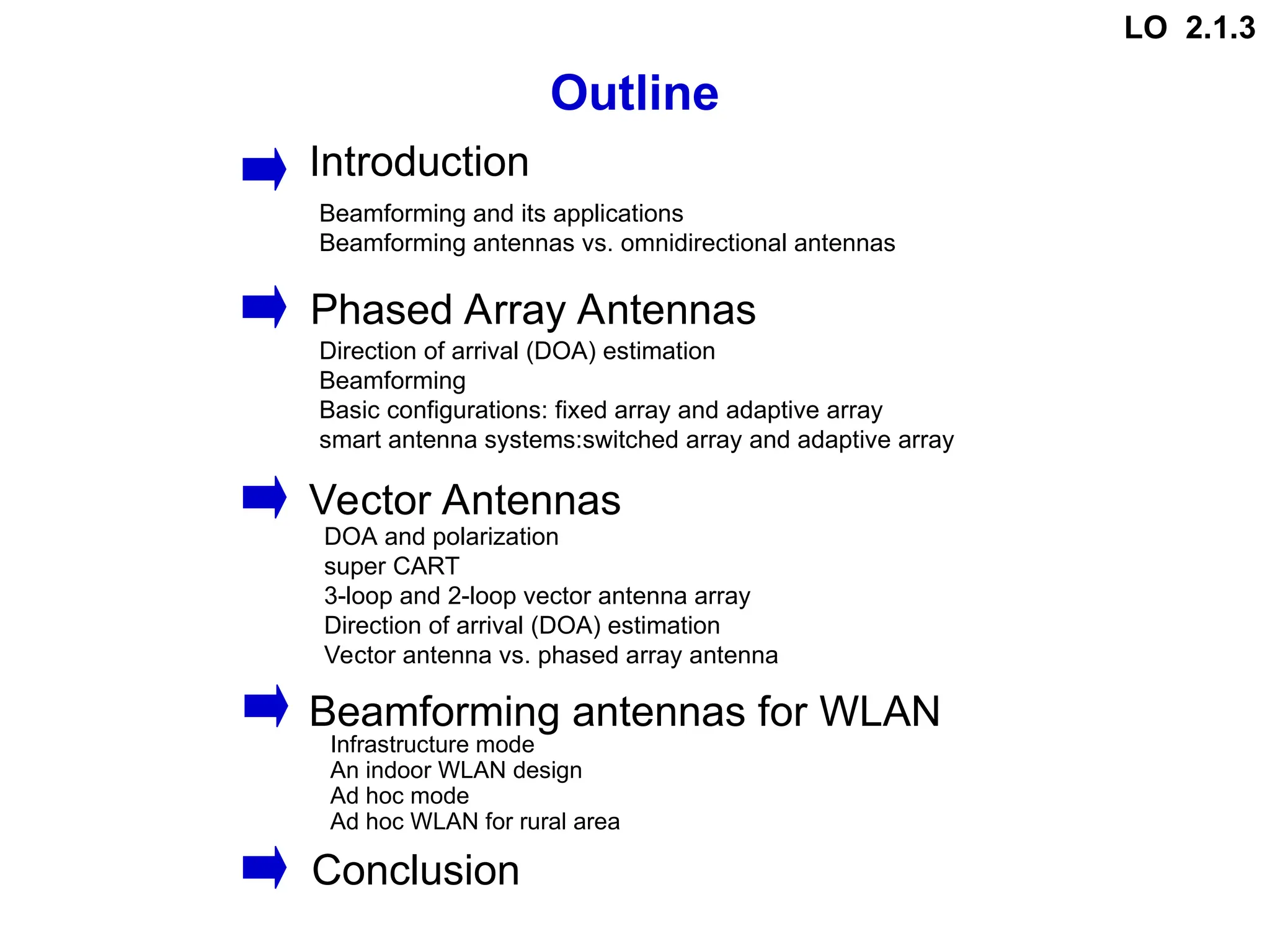
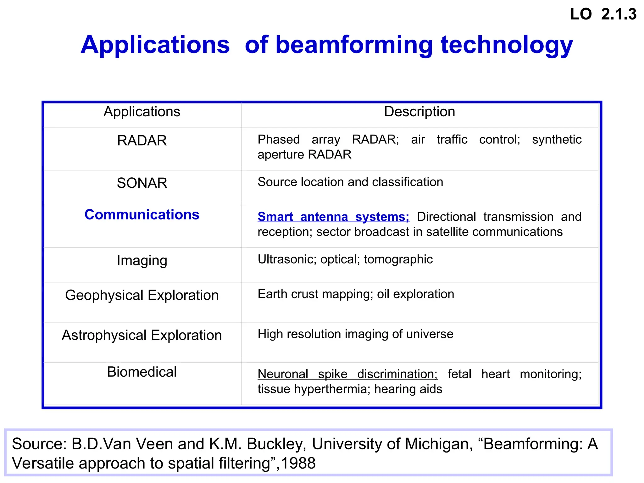
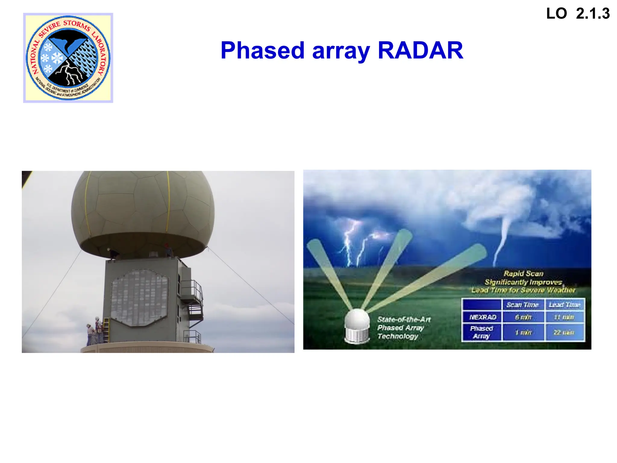
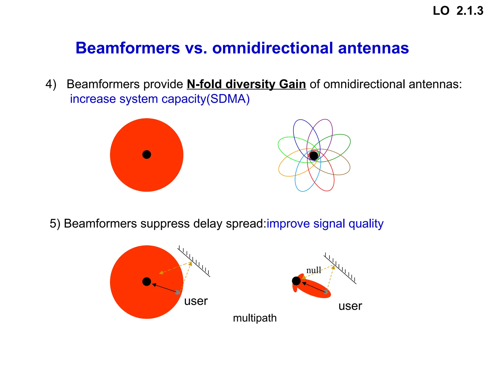
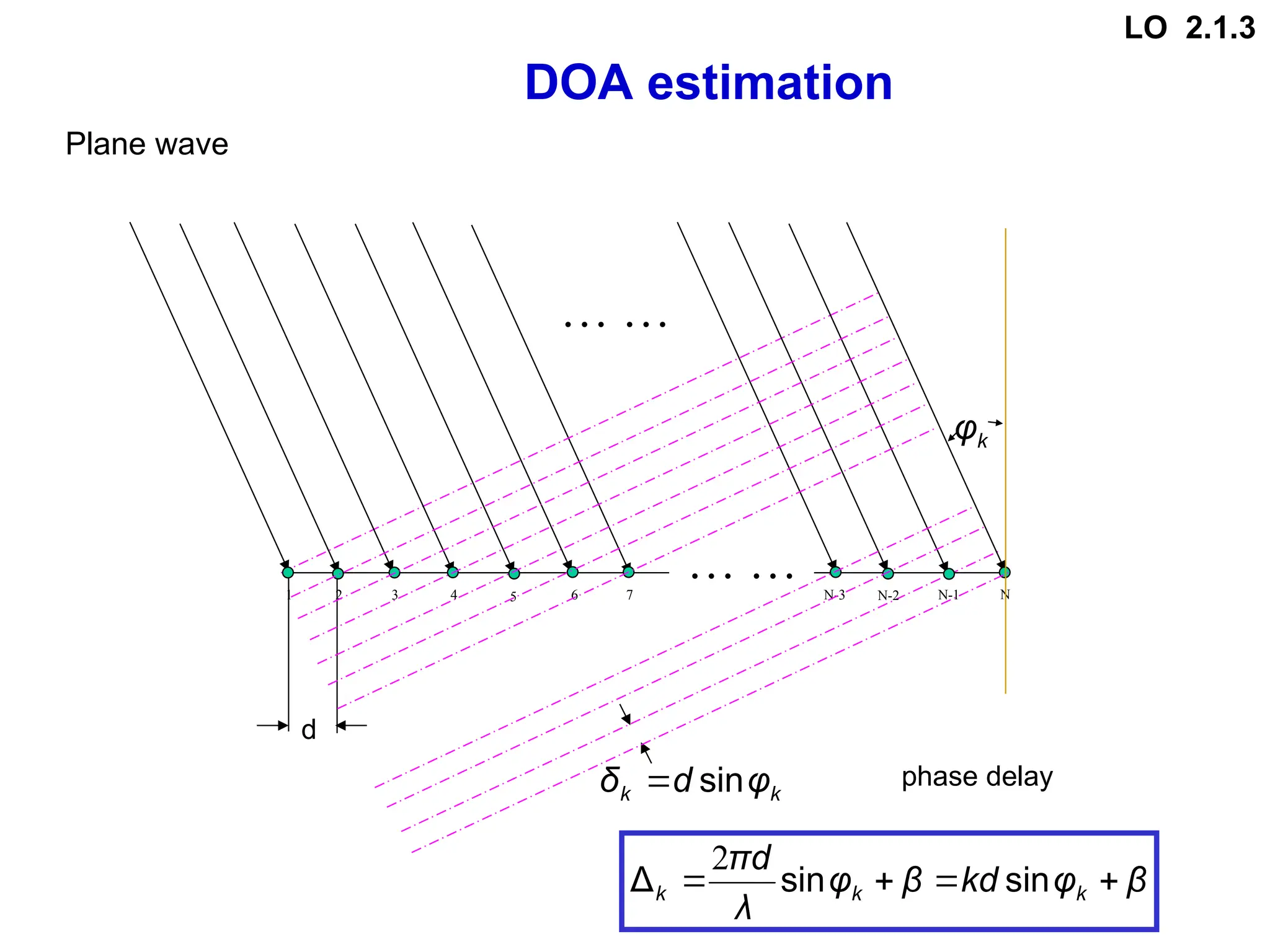
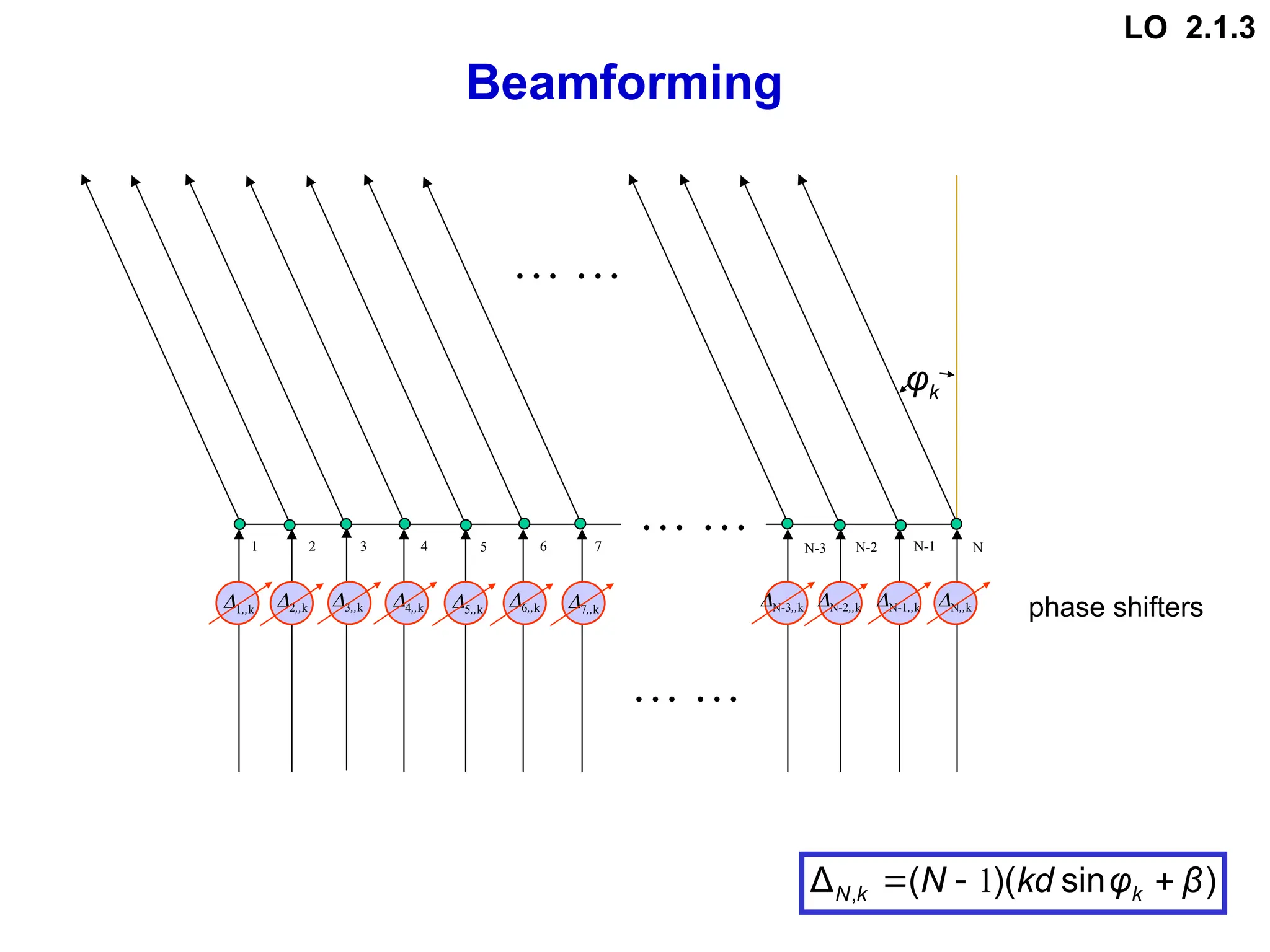
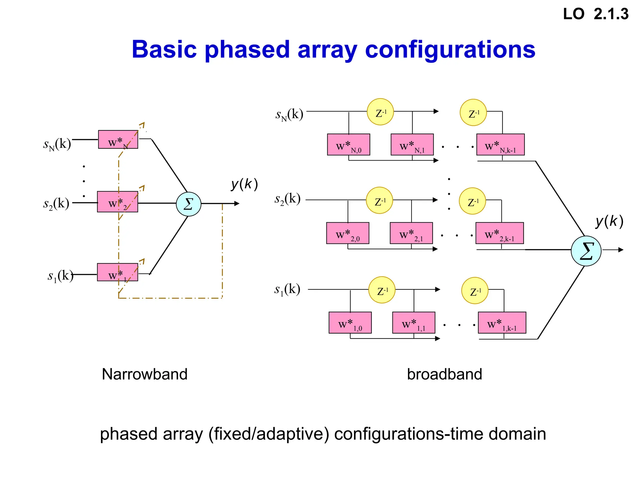
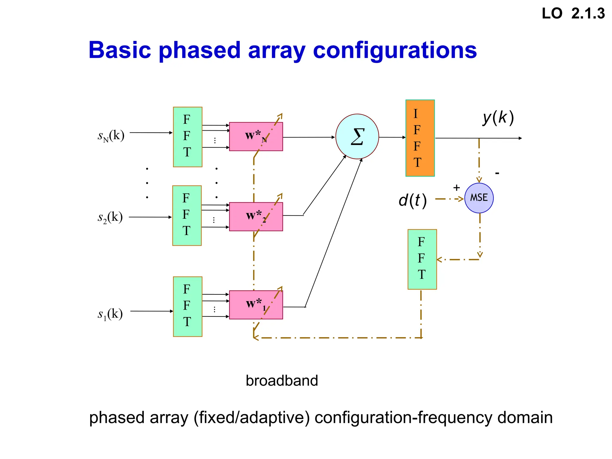
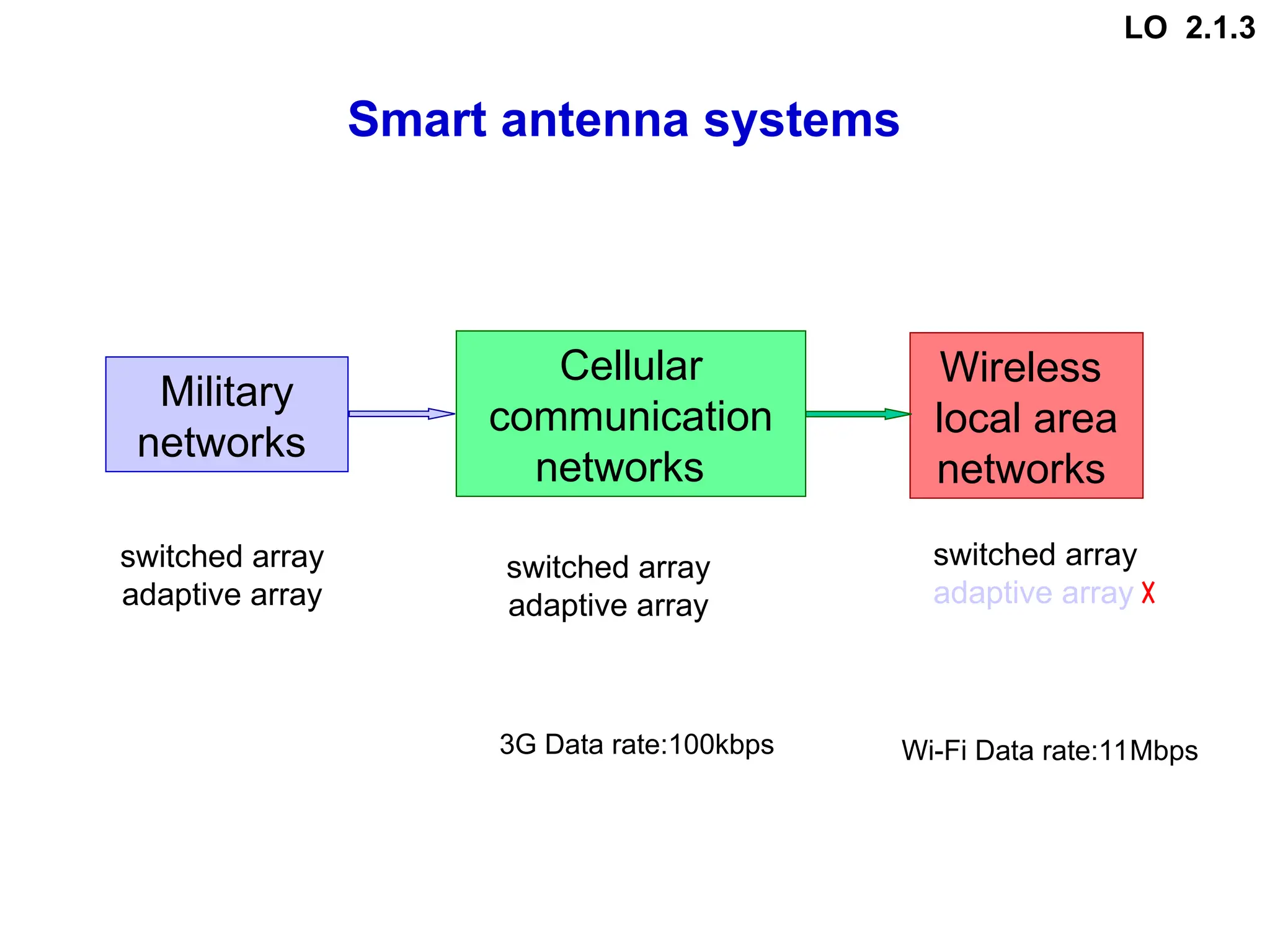
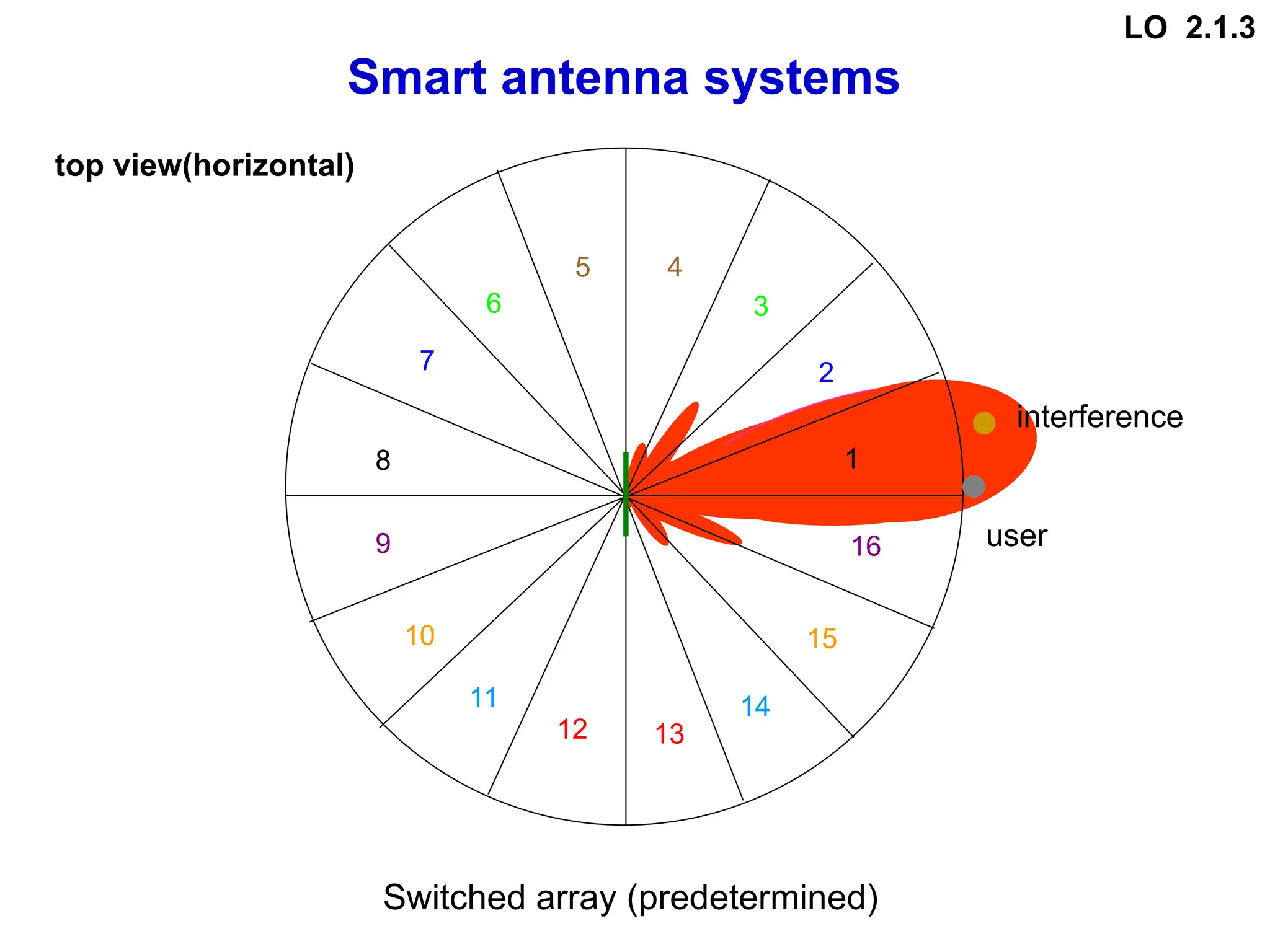
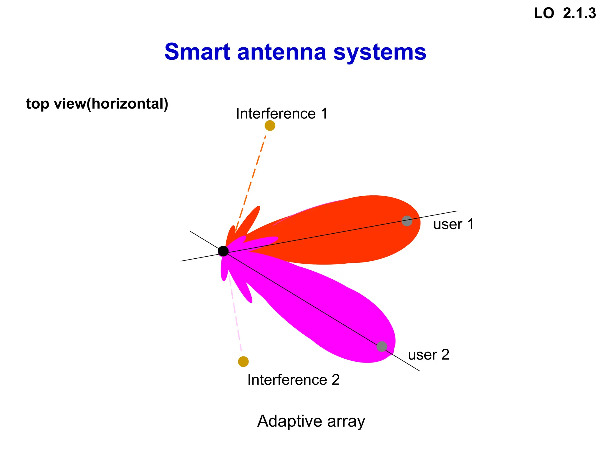
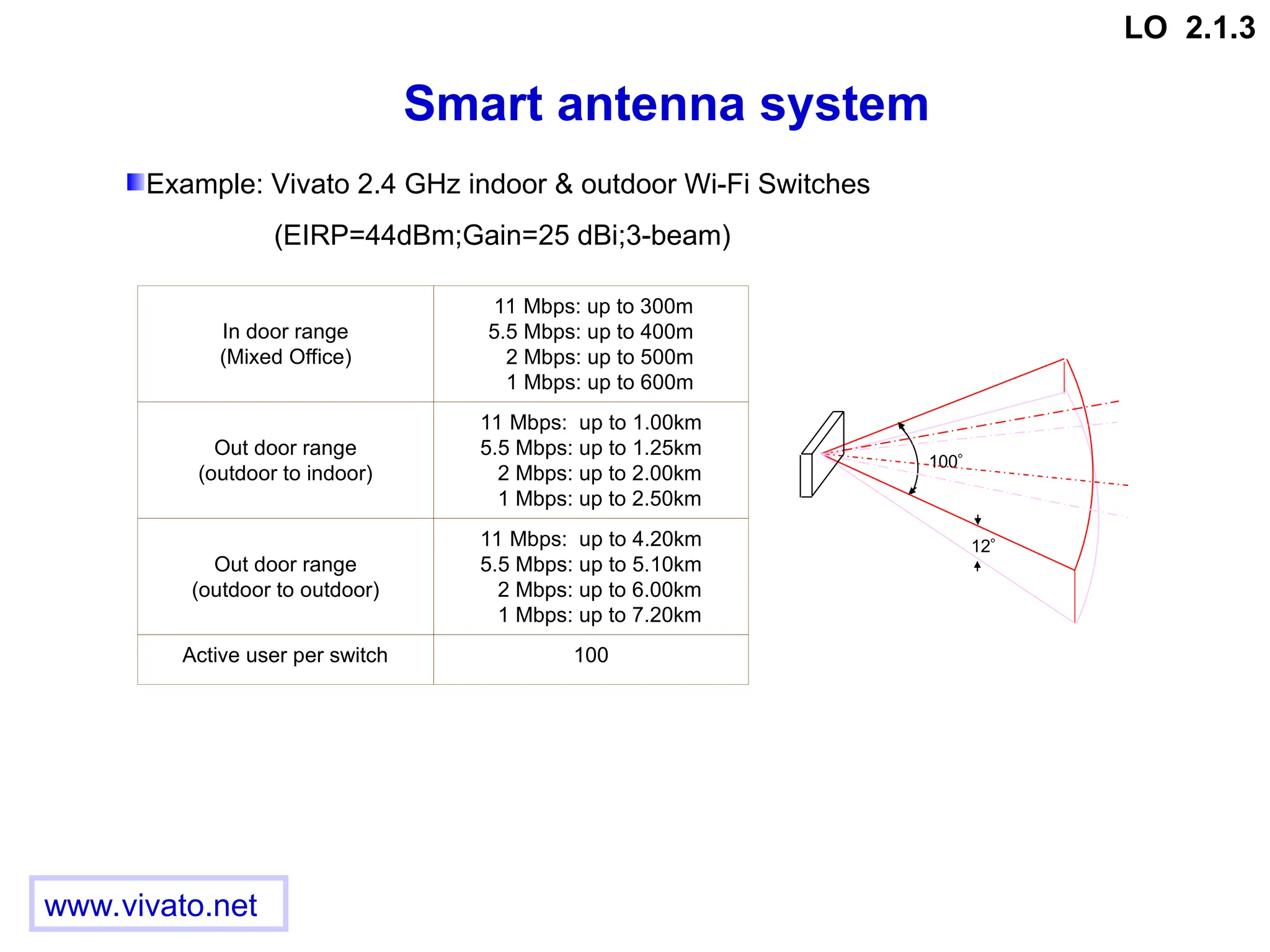
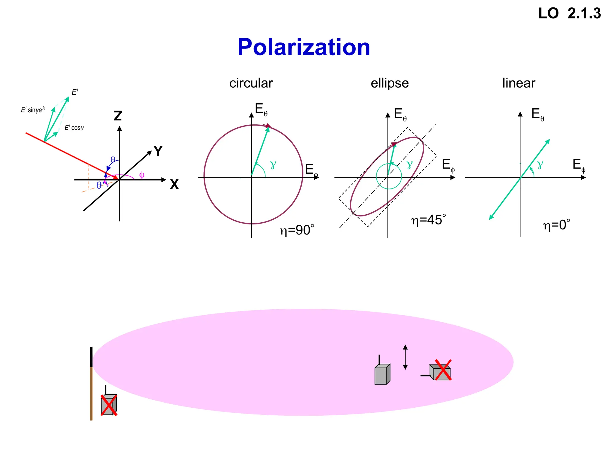
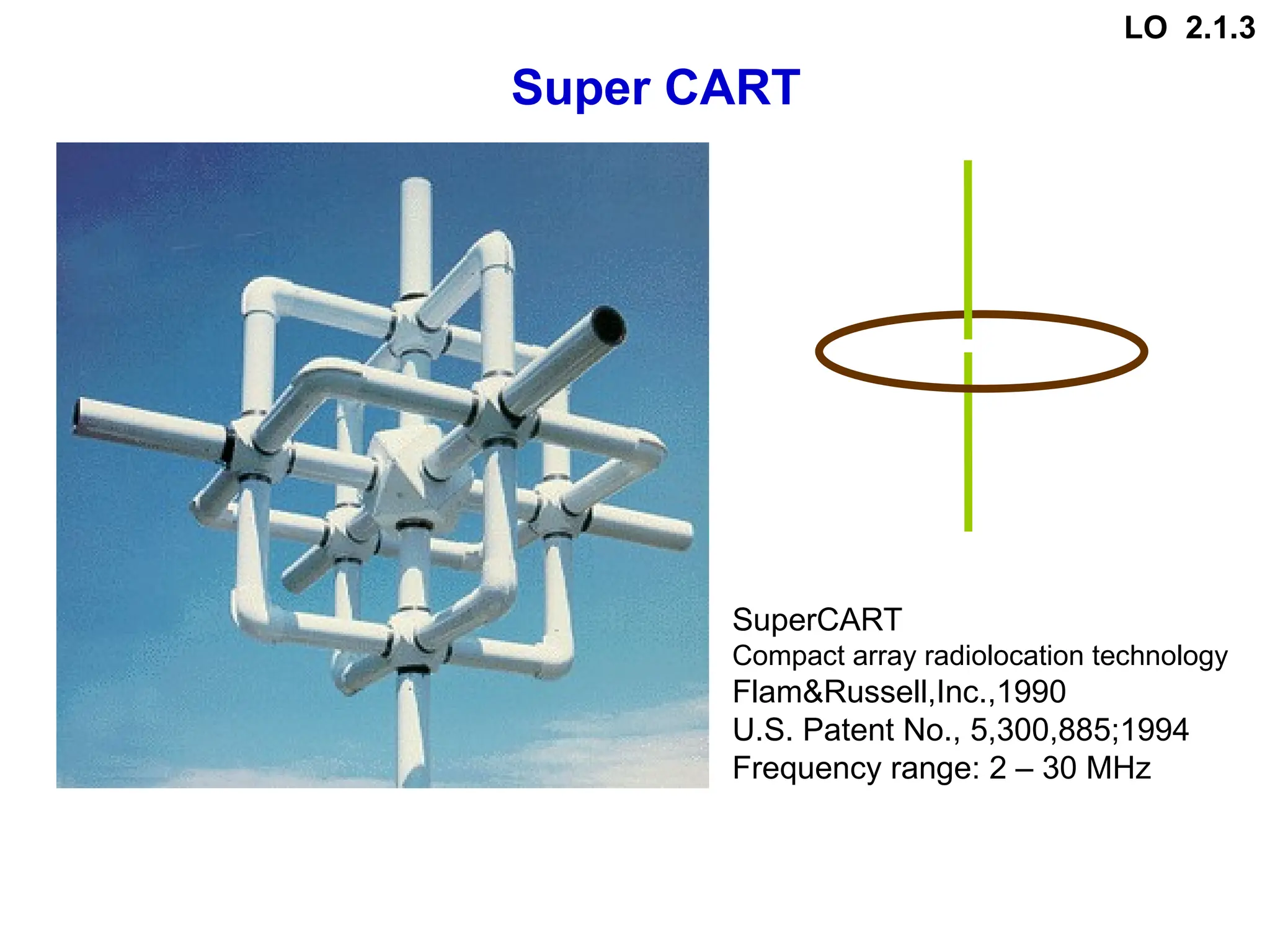
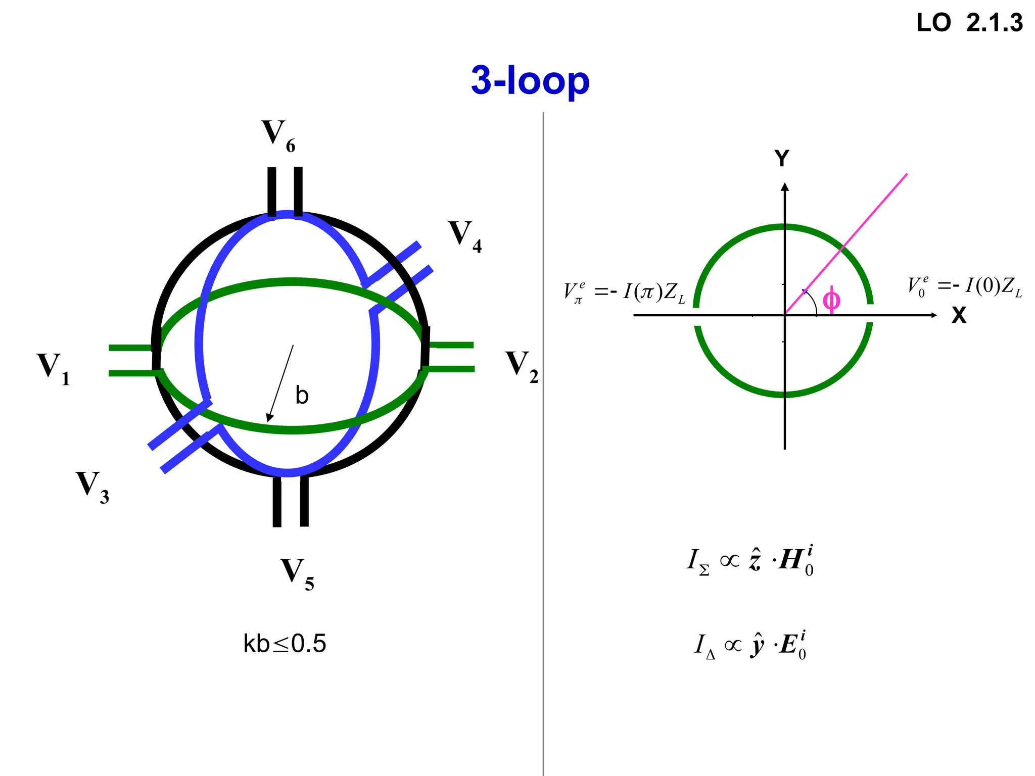
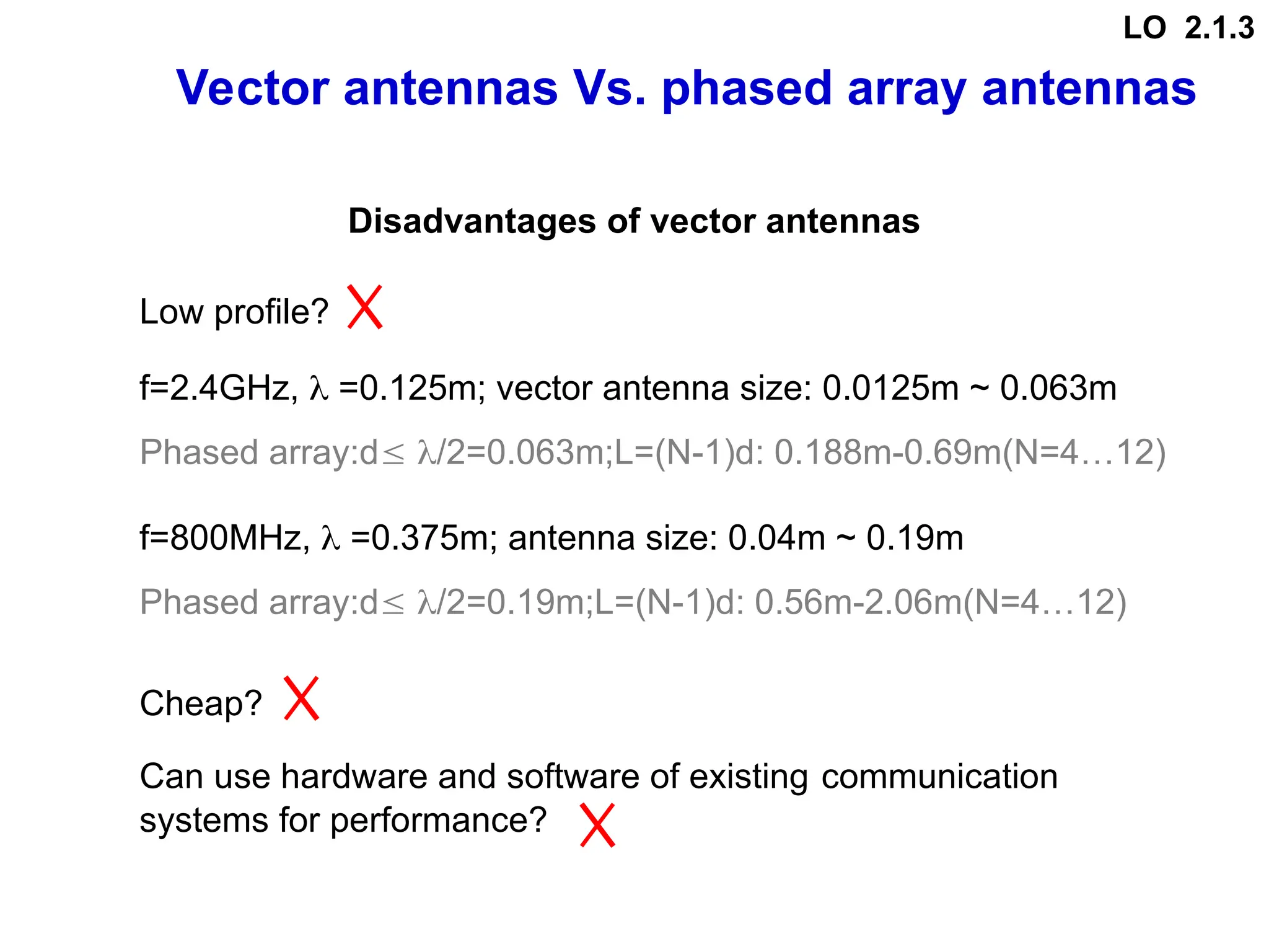
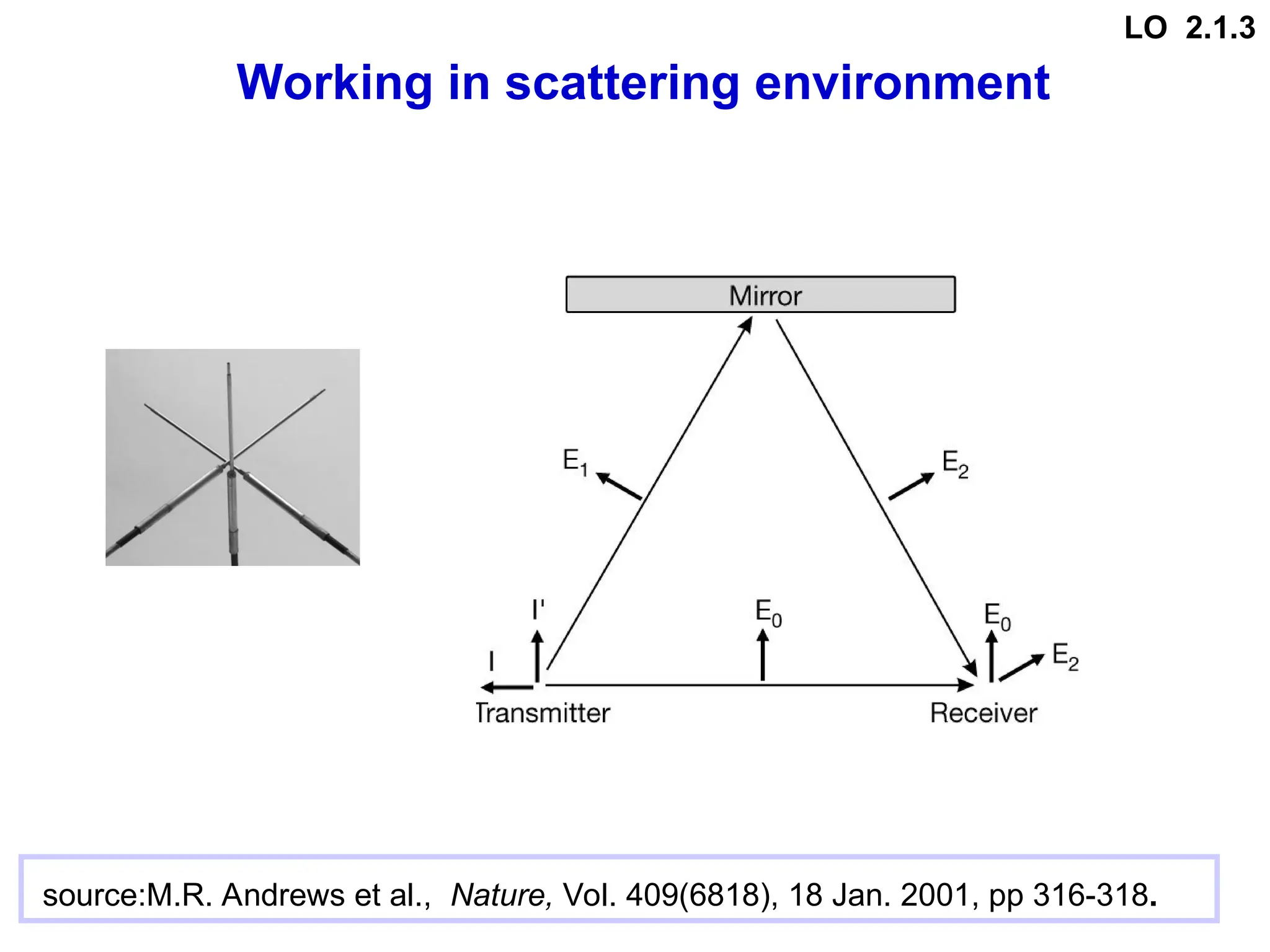
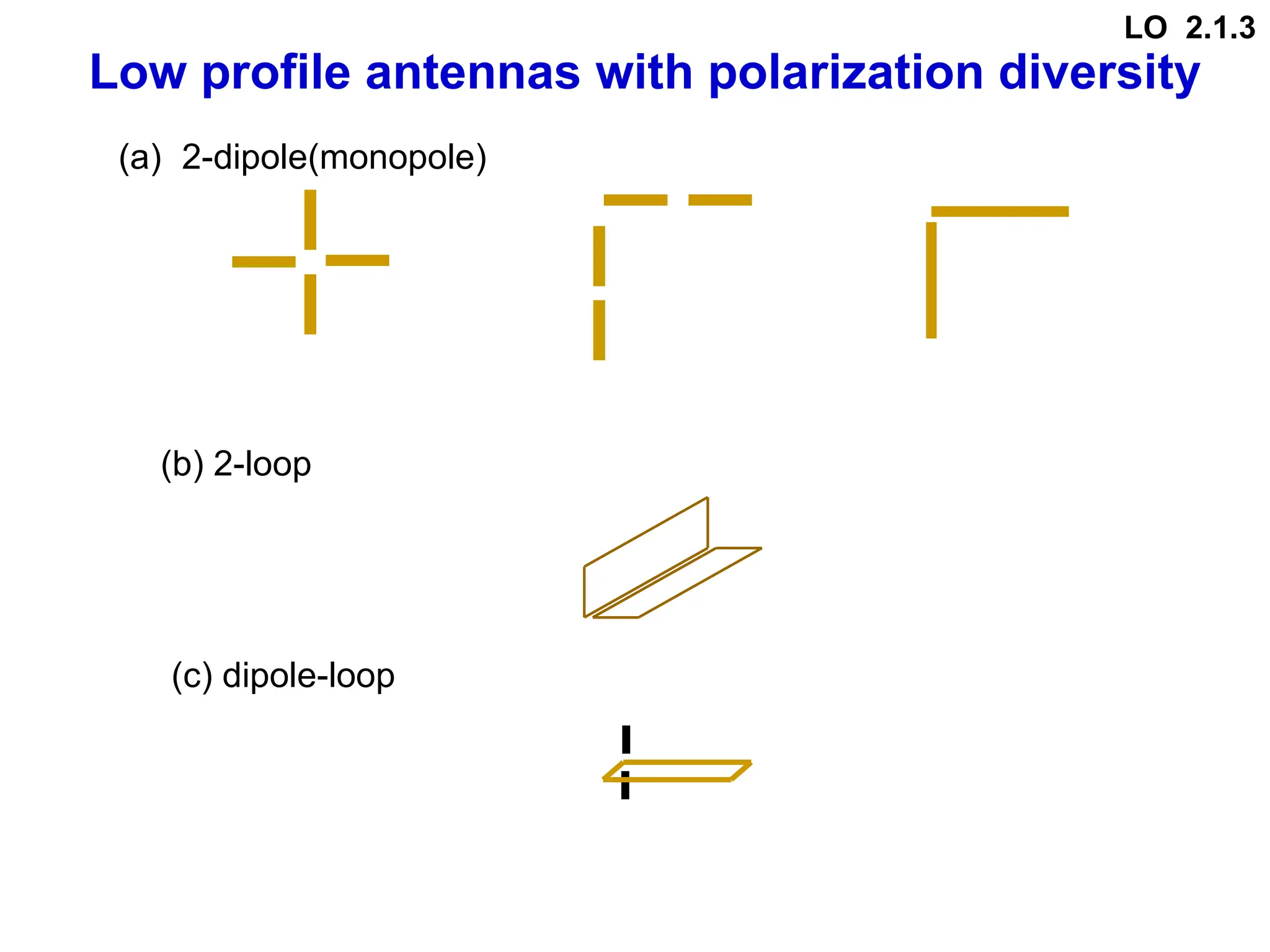
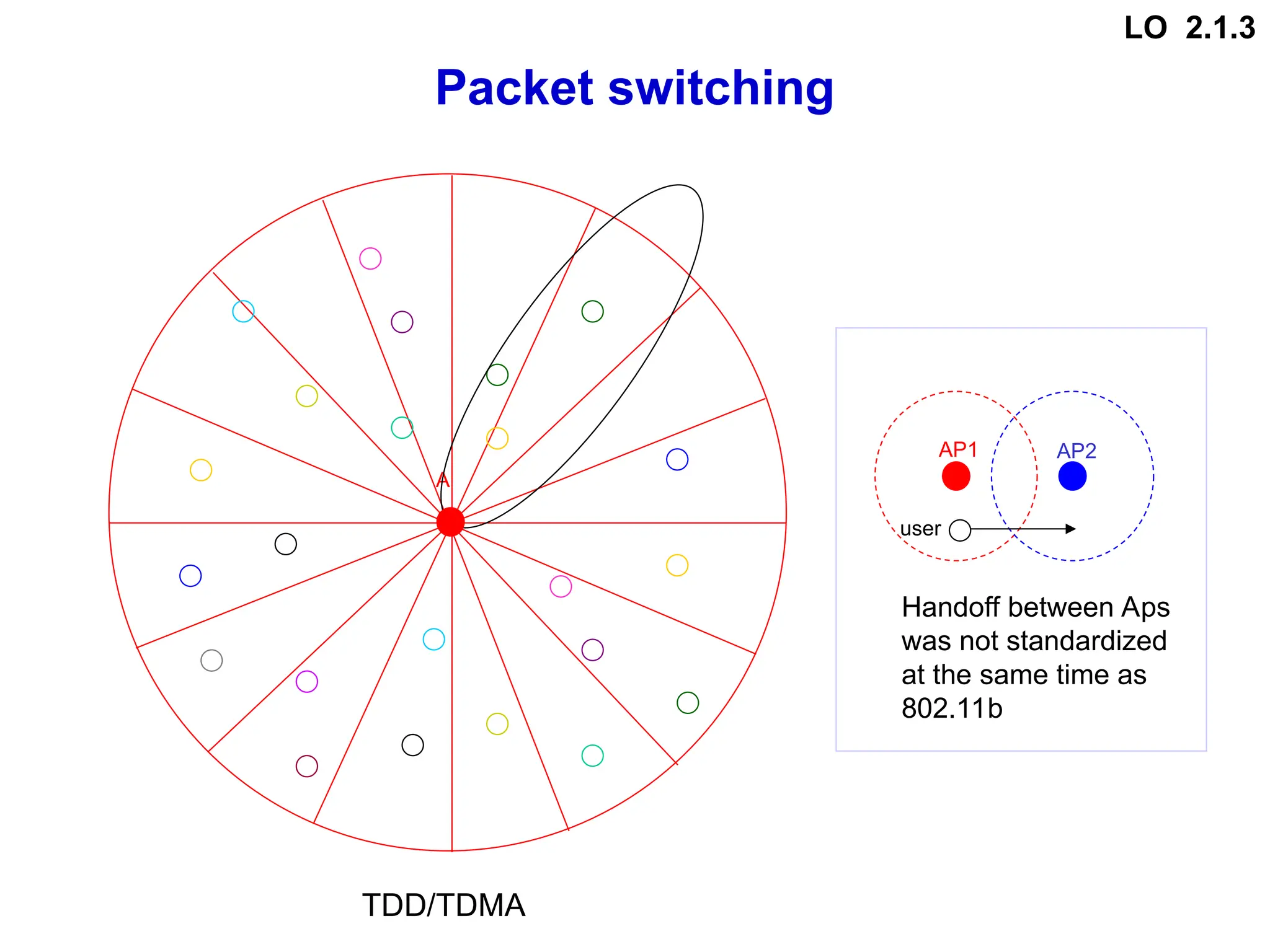
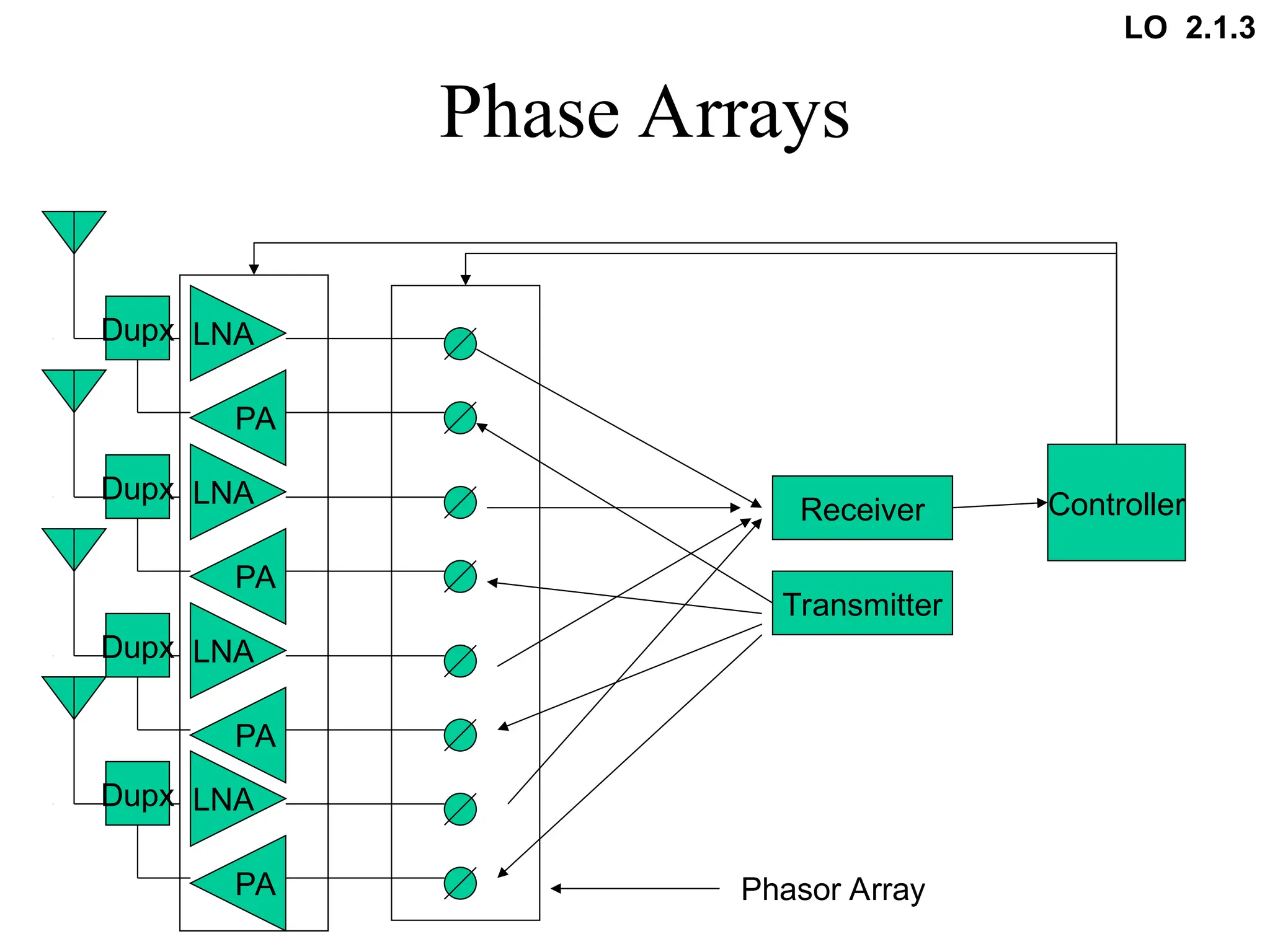
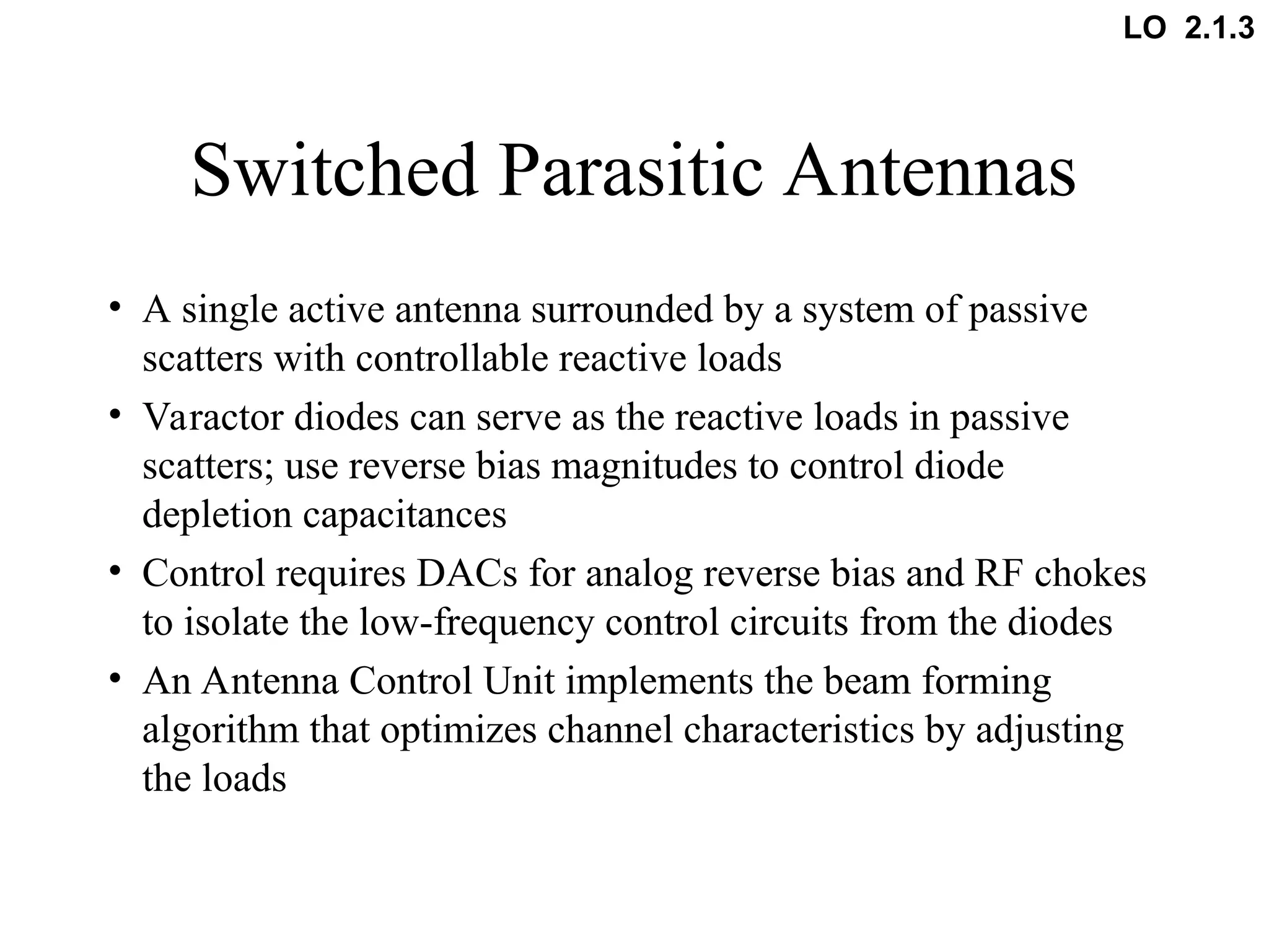
1. Beamforming Antennas
LO 2.1.3

2. Outline
Phased Array Antennas
Vector Antennas
Beamforming antennas for WLAN
Conclusion
Introduction
Beamforming and its applications
Beamforming antennas vs. omnidirectional antennas
Direction of arrival (DOA) estimation
Beamforming
Basic configurations: fixed array and adaptive array
smart antenna systems:switched array and adaptive array
DOA and polarization
super CART
3-loop and 2-loop vector antenna array
Direction of arrival (DOA) estimation
Vector antenna vs. phased array antenna
Infrastructure mode
An indoor WLAN design
Ad hoc mode
Ad hoc WLAN for rural area
LO 2.1.3

3. Applications Description
RADAR Phased array RADAR; air traffic control; synthetic
aperture RADAR
SONAR Source location and classification
Communications Smart antenna systems; Directional transmission and
reception; sector broadcast in satellite communications
Imaging Ultrasonic; optical; tomographic
Geophysical Exploration Earth crust mapping; oil exploration
Astrophysical Exploration High resolution imaging of universe
Biomedical Neuronal spike discrimination; fetal heart monitoring;
tissue hyperthermia; hearing aids
Source: B.D.Van Veen and K.M. Buckley, University of Michigan, “Beamforming: A
Versatile approach to spatial filtering”,1988
Applications of beamforming technology
LO 2.1.3

4. Phased array RADAR
LO 2.1.3

5. Phased array spike sorting
0.139
0.544

Ey1n t
( )
1.2 10
4

0 t
0.056
0.205

Ey2n t
( )
1.2 10
4

0 t
0.042
0.187

Ey3n t
( )
1.2 10
4

0 t
Sorted
Spike of
individual
neurons.
1
2
3
4
1
6
5
6
7
8
9
1
4
1
5
1
3
1
2
1
1
1
0
0.139
0.534

Rn 3 t

( )
1.2 10
4

0 t
0.183
0.539

Rn 5 t

( )
1.2 10
4

0 t
0.147
0.534

Rn 7 t

( )
1.2 10
4

0 t
0.147
0.534

Rn 9 t

( )
1.2 10
4

0 t
0.183
0.539

Rn 11 t

( )
1.2 10
4

0 t
0.139
0.534

Rn 13 t

( )
1.2 10
4

0 t
0.14
0.534

Rn 1 t

( )
1.2 10
4

0 t
0.148
0.534

Rn 15 t

( )
1.2 10
4

0 t
Neuronal
spikes
recorded by
electrode
array
Phased
array
spike
sorting
system
Center for Computational Biology, MSU
LO 2.1.3

6. Patterns, beamwidth & Gain
Isotropic dipole
top
view(horizontal)
side
view(vertical)
half-wave dipole beamformer
2
1/
φ
Half-power
beam width
Half-power
beam width
Half-power
beam width
Main lobe
side lobes
nulls
2
1/
θ
78°
LO 2.1.3

7. Beamformers vs. omnidirectional antennas
1) Beamformers have much higher Gain than omnidirectional antennas:
Increase coverage and reduce number of antennas!
Gain:
2
1
N
G
GN

0
30
60
90
120
150
180
210
240
270
300
330
6
4
2
0
6
9.961 10
7


Field 6 0
 

( )
Field 2 0
 

( )
Field 1 0
 

( )

LO 2.1.3

8. Beamformers vs. omnidirectional antennas
2) Beamformers can reject interference while omnidirectional
antennas can’t: Improve SNR and system capacity!
3) Beamformers directionally send down link information to the
users while omnidirectional antennas can’t: save energy!
user
interference
user
interference
null
LO 2.1.3

9. Beamformers vs. omnidirectional antennas
user user
null
multipath
4) Beamformers provide N-fold diversity Gain of omnidirectional antennas:
increase system capacity(SDMA)
5) Beamformers suppress delay spread:improve signal quality
LO 2.1.3

10. DOA estimation
β
φ
kd
β
φ
λ
d
π
k
k
k 


 sin
sin
Δ
2
phase delay
1 2 3 4 5 6 7 N
N-2 N-1
N-3
… …
… …
d
k
k φ
d
δ sin

k
φ
Plane wave
LO 2.1.3

11. Beamforming
phase shifters
1 2 3 4 5 6 7 N
N-2 N-1
N-3
… …
… …
k
φ
… …
1,,k
2,,k 3,,k 4,,k 5,,k
6,,k 7,,k
N-3,,k N-2,,k N-1,,k N,,k
)
sin
)(
(
Δ , β
φ
kd
N k
k
N 

 1
LO 2.1.3

12. phased array (fixed/adaptive) configurations-time domain
Basic phased array configurations
Narrowband
sN(k)
s2(k)
s1(k)
.
.
.
w*N
w*2
w*1

)
(k
y
broadband
sN(k)
s2(k)
s1(k)
.
.
.

)
(k
y
w*N,0 w*N,1 w*N,k-1
.
.
.
Z-1
Z-1
w*2,0 w*2,1 w*2,k-1
.
.
.
Z-1
Z-1
w*1,0 w*1,1 w*1,k-1
.
.
.
Z-1
Z-1
LO 2.1.3

13. phased array (fixed/adaptive) configuration-frequency domain
Basic phased array configurations
…
…
…
sN(k)
s2(k)
s1(k)
.
.
.
-
+
I
F
F
T
MSE
F
F
T
w*N
w*2
w*1

)
(k
y
)
(t
d
F
F
T
F
F
T
F
F
T
broadband
.
.
.
LO 2.1.3

14. Smart antenna systems
Military
networks
Cellular
communication
networks
Wireless
local area
networks
switched array
adaptive array
switched array
adaptive array
switched array
adaptive array
Wi-Fi Data rate:11Mbps
3G Data rate:100kbps
LO 2.1.3

15. Switched array (predetermined)
top view(horizontal)
Smart antenna systems
interference
user
1
2
3
4
5
6
7
8
9
10
11
12 13
14
15
16
LO 2.1.3

16. user 1
Interference 1
top view(horizontal)
user 2
Smart antenna systems
Interference 2
Adaptive array
LO 2.1.3

17. Smart antenna system
www.vivato.net
12
100
In door range
(Mixed Office)
11 Mbps: up to 300m
5.5 Mbps: up to 400m
2 Mbps: up to 500m
1 Mbps: up to 600m
Out door range
(outdoor to indoor)
11 Mbps: up to 1.00km
5.5 Mbps: up to 1.25km
2 Mbps: up to 2.00km
1 Mbps: up to 2.50km
Out door range
(outdoor to outdoor)
11 Mbps: up to 4.20km
5.5 Mbps: up to 5.10km
2 Mbps: up to 6.00km
1 Mbps: up to 7.20km
Active user per switch 100
Example: Vivato 2.4 GHz indoor & outdoor Wi-Fi Switches
(EIRP=44dBm;Gain=25 dBi;3-beam)
LO 2.1.3

18. Polarization
circular
E

linear
=0
E
E

ellipse
=45
X
Y
Z
i
E

η
j
i
e
γ
E sin
γ
Ei
cos

’
E

E
=90
E
LO 2.1.3

19. SuperCART
Compact array radiolocation technology
Flam&Russell,Inc.,1990
U.S. Patent No., 5,300,885;1994
Frequency range: 2 – 30 MHz
Super CART
LO 2.1.3

20. 3-loop
V6
V4
V3
V1
V2
V5
Y
X
 L
e
Z
I
V )
0
(
0 

L
e
Z
I
V )
(
 

i
H
z 0
ˆ




I
i
E
y 0
ˆ




I
kb0.5
b
LO 2.1.3

21. 2-loop
H
E
S
Steering vector




































γ
γ
a
η
cos
e
sin
Θ
sin
Θ
cos
Φ
cos
Φ
sin
Θ
sin
Φ
cos
Θ
cos
Φ
sin
h
h
e
e
j
z
x
z
y
0
0
0
0
0
0
0
4
ζ
H
i
i E0
0 
1
2
2
2


 z
y
x e
e
e
1
2
2
2


 z
y
x h
h
h
Blind point
LO 2.1.3

22. Vector antennas vs. spatial array antennas
Vector antennas measure: ,,,, and power simultaneously,
no phase shift device, or synchronization is needed.
Phased array antennas with omnidirectional element measure:
,, and power
LO 2.1.3

23. Source: Nehorai,A.,University of Illinois at Chicago
Vector antennas vs. spatial array antennas
VA
SA
VA SA
LO 2.1.3

24. Vector antennas vs. spatial array antennas
Phased array antennas: spatial ambiguities exist
2
2
1
1 φ
f
φ
f sin
sin 
1 2 3 4 5 6 7
… …
k
φ
k
φ
1 2 3 4 5 6 7
… …
1
φ
2
φ
P
η
γ
θ
φ ,
,
,
,
h
,
h
,
h
,
e
,
e
,
e z
y
x
z
y
x 
Vector antenna: no ambiguities for DOA estimation
LO 2.1.3

25. Vector antennas Vs. phased array antennas
Disadvantages of vector antennas
Cheap?
Can use hardware and software of existing communication
systems for performance?
f=2.4GHz,  =0.125m; vector antenna size: 0.0125m ~ 0.063m
Phased array:d /2=0.063m;L=(N-1)d: 0.188m-0.69m(N=4…12)
f=800MHz,  =0.375m; antenna size: 0.04m ~ 0.19m
Phased array:d /2=0.19m;L=(N-1)d: 0.56m-2.06m(N=4…12)
Low profile?
LO 2.1.3

26. source:M.R. Andrews et al., Nature, Vol. 409(6818), 18 Jan. 2001, pp 316-318.
Working in scattering environment
LO 2.1.3

27. (a) 2-dipole(monopole)
Low profile antennas with polarization diversity
(c) dipole-loop
(b) 2-loop
LO 2.1.3

28. TDD/TDMA
Packet switching
A
AP1 AP2
user
Handoff between Aps
was not standardized
at the same time as
802.11b
LO 2.1.3

29. Packet switching: 3 beam system
top view(horizontal)
i
i
i
P
P
P
d 1
1 
 

P. Sanchis, et al. 02
i
P
1

i
P
1

i
P
φ
Δ
φ
Δ
 
 


















1
2
2
1
1
2
1
2
2
1
d
φ
d
φ
d
φ
d
φ
d
φ
d
φ
φ
i
i
i
DOA
),
/
Δ
(
/
),
/
Δ
(
),
/
Δ
(
/
ˆ
max
max
max
LO 2.1.3

30. An indoor WLAN design
A 4-story office building (including basement), high 30 m, wide 60m and long 100m. We
plan to install a Vivato switched array on the 3rd floor.
L=100m
h=30m
w=60m
Switched array
3
2
1
Basement
LO 2.1.3

31. An indoor WLAN design
Data rate 1Mbps, 2Mbps, 5.5Mbps, 11Mbps
AP’s EIEP 44dBm
AP’s antenna Gain GA 25 dBi
PC antenna Gain GP 0 dBi
Shadowing 8dB
AP’s antenna receiving sensitivity Smin -95dBm ,-92dBm, ,-89dBm, -86dBm
AP’s Noise floor -178dBm/Hz
Body/orientation loss 2dB
Soft partition attenuate factor (p= number) p1.39 dB
Concrete-wall attenuate factor(q= number) q2.38 dB
Average floor attenuation(floor number) 14.0dB(1),19.0dB(2),23.0dB(3),26.0dB(4)
Frequency 2.4GHz
Reference pathloss PL0 (LOS/NLS, r=1m) 45.9dB/ 50.3dB
Pathloss exponent  (LOS/NLS, r=1m) 2.1/3.0
Pathloss standard deviation  (LOS/NLS) 2.3dB/4.1dB
Average floor attenuation(floor number) 14.0dB(1),19.0dB(2),23.0dB(3),26.0dB(4)
Data of AP’s antenna is from www.vivato.net
LO 2.1.3

32. An indoor WLAN design
Mean pathloss with smin:
P
G
S
EIRP
L 

 min
o
sd
fl
sm
w
allowable L
L
L
L
L
L
PL 





Path loss model: )
log(
)
(
0
0 10
r
r
γ
PL
r
PL 

al
PL
r
PL 
)
(
The coverage ranges are:r=36m,29m,23m and 18m for date rate at 1Mbps, 2Mbps,
5.5Mbps and 11Mbps respectively
Allowable pathloss:
Case 1: user is on the 3rd
floor: 3 concrete walls, 3 soft partitions
The coverage ranges are: r=176m,140m,111m and 88m for date rate at 1Mbps,
2Mbps, 5.5Mbps and 11Mbps respectively .
Case 2: user is in the basement : 3 floors; 2 concrete walls, 3 soft partitions
LO 2.1.3

33. Beamforming antennas in ad hoc networks
P.Gupta and P.R. Kumar,00
throughput
obtained
by
each
node








n
nlog
W
~
Beam-
forming
antennas
?
new
routing
protocol
new
channel
access
scheme
LO 2.1.3

34. Beamforming antennas in ad hoc networks
interference
target
Phased patch
antenna
D.Lu and D.Rutledge,Caltech,02
Z0=50
Z0=50,L/
2
Z0=25,L/
2
Series resonant patch array
Phased patch array
LO 2.1.3

35. Beamforming antennas in ad hoc networks
Medium Access Control Protocol(CSMA/CA)
CSMA/CA:carrier sense multiple access/collision avoidance
( for omnidirectional antennas)
(Scheduled/On-demand)
Packet routing
Neighbor discovery
 No standard MAC protocols for directional antenna
 Ad hoc networks may achieve better performance in some cases
using beamforming antennas.
 No obvious improvement for throughput using beamforming antennas
 Neighbor discovery become more complex using beamforming antennas.
 Beamforming antennas can significantly increasing node and
network lifetime in ad hoc networks.
LO 2.1.3

36. 1) traditional exposed node
problem for omnidirectional
antennas
Channel access
Source:Y Ko et al., 00
A B C D E
RTS
CTS
DATA
ACK
RTS
CTS
DATA
DATA
DATA
ACK
A B C D E
RTS
CTS CTS
DATA
DATA
ACK
RTS
CTS CTS
DATA
DATA
ACK
1) No coverage change. May save power.
2) B may not know the location of C.
The nodes
are
prohibit to
transmit or
receive
signals
The node
is free to
transmit or
receive
signals
The node is
blocked to
communicat
e with C
2) Omnidirectional and
directional antennas solve
the exposed node problem
LO 2.1.3

37. Channel access
A B C D E
RTS
CTS
CTS
DATA
RTS
collision
deaf
collision
A B C D E
RTS
CTS
DATA
DATA
RTS
3) beamforming antennas create new problems
LO 2.1.3

38. Neighbor discovery
A
B
C
D
E
A
t
Nt
“Hello”
AP Neighbors
A B,C
B A,C
C A,B,E
D E
E C,D
LO 2.1.3

39. Ad hoc WLAN for rural area
LO 2.1.3

40. Conclusion
Beamforming antenna systems improve wireless
network performance
-increase system capacity
-improve signal quality
-suppress interference and noise
-save power
Beamforming antennas improve infrastructure
networks performance. They may improve ad hoc
networks performance. New MAC protocol
standards are needed.
Vector antennas may replace spatial arrays to
further improve beamforming performance
LO 2.1.3

41. Phase Arrays
PA
LNA
PA
LNA
PA
LNA
PA
LNA
Transmitter
Receiver Controller
Phasor Array
Dupx
Dupx
Dupx
Dupx
LO 2.1.3

42. Switched Parasitic Antennas
• A single active antenna surrounded by a system of passive
scatters with controllable reactive loads
• Varactor diodes can serve as the reactive loads in passive
scatters; use reverse bias magnitudes to control diode
depletion capacitances
• Control requires DACs for analog reverse bias and RF chokes
to isolate the low-frequency control circuits from the diodes
• An Antenna Control Unit implements the beam forming
algorithm that optimizes channel characteristics by adjusting
the loads
LO 2.1.3