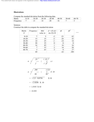
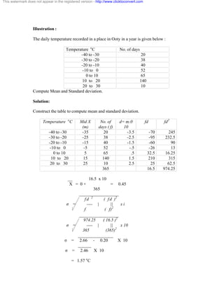
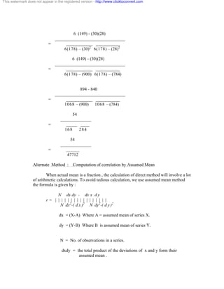
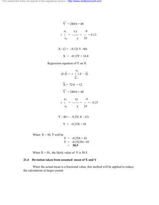
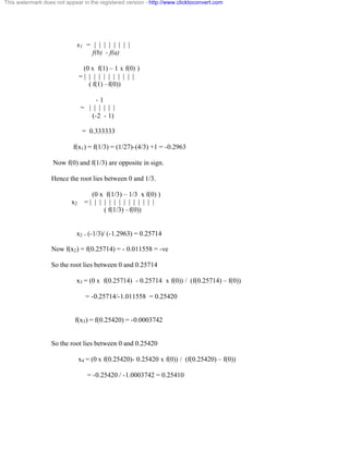
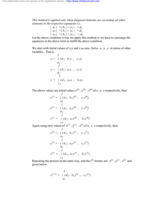
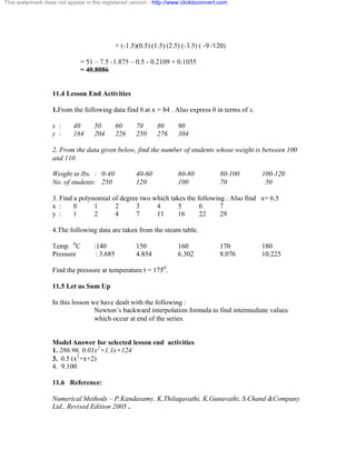
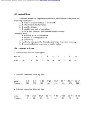
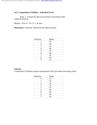
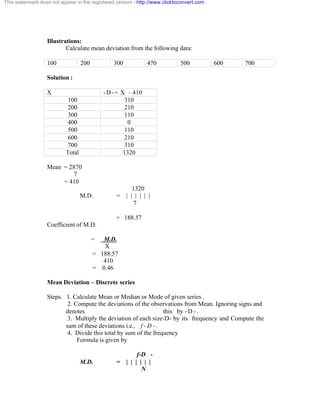
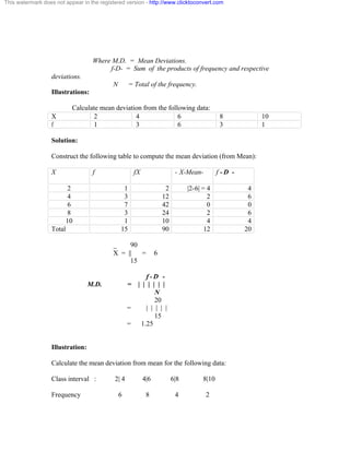
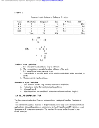
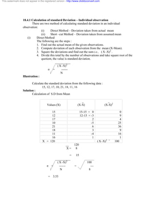
This document discusses methods for solving numerical equations, including the bisection method, Newton-Raphson method, and method of false position. It provides definitions and step-by-step computations for each method. For the bisection method, it gives an example of finding the positive root of x3 - x = 1. For Newton-Raphson, it gives examples of finding the root of 2x3 - 3x - 6 = 0 and x3 = 6x - 4. The document serves to introduce numerical methods for solving equations.
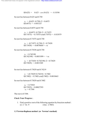
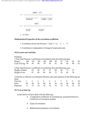
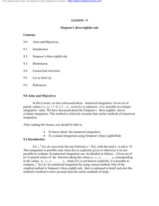
![This watermark does not appear in the registered version - http://www.clicktoconvert.com
X2 = (2(2/3)
3 – 4 )/(3(2/3)
2-6) = 0.73016
X3 = (2(0.73015873)
3 – 4 )/(3(0.73015873)
2-6)
= (3.22145837/ 4.40060469)
= 0.73205
X4 = (2(0.73204903)
3 – 4 )/(3(0.73204903)
2-6)
= (3.21539602/ 4.439231265)
= 0.73205
The root is 0.73205 correct to 5 decimal places.
Check Your Progress :
Solve the following by using Newton – Raphson Method :
x3 -x -1 (Ans :1.3247 )
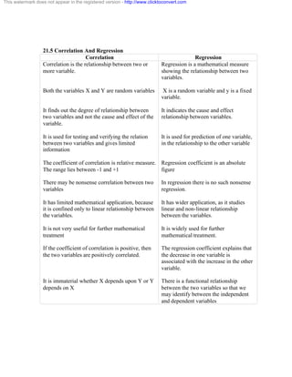
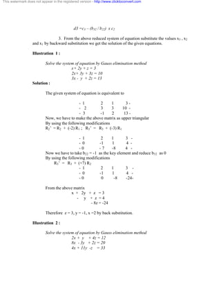
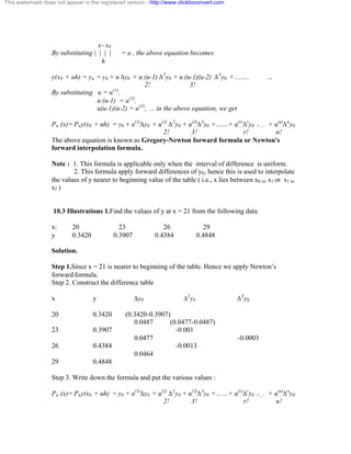
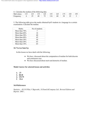
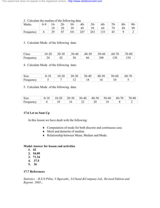
1.4 Method of False Position ( or Regula Falsi Method )
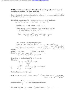
Consider the equation f(x) = 0 and f(a) and f(b) are of opposite signs. Also let a< b.
The graph y = f(x) will Meet the x-axis at some point between A(a, f(a)) and
B (b,f(b)). The equation of the chord joining the two points A(a, f(a)) and
B (b,f(b)) is
y – f(a) f(a) - f(b)
||||| = | | | | | | |
x - a a - b
The x- Coordinate of the point of intersection of this chord with the x-axis gives an
approximate value for the of f(x) = 0. Taking y = 0 in the chord equation, we get
– f(a) f(a) - f(b)
||||| = | | | | | | |
x - a a - b
x[f(a) - f(b)] - a f(a) + a f(b) = -a f(a) + b f(b)
x[f(a) - f(b)] = b f(a) - a f(b)
This x1 gives an approximate value of the root f(x) = 0. (a < x1 < b)
Now f(x1) and f(a)are of opposite signs or f(x1) and f(b) are opposite signs.
If f(x1 ), f(a) <0 . then x2 lies between x1 and a.](https://image.slidesharecdn.com/bcanumer-141110101906-conversion-gate02/85/Bca-numer-8-320.jpg)
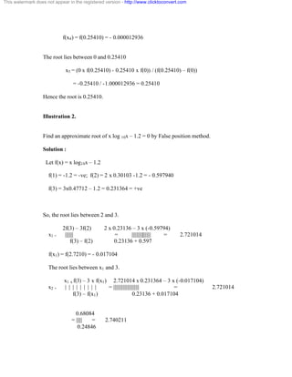
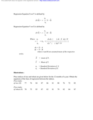
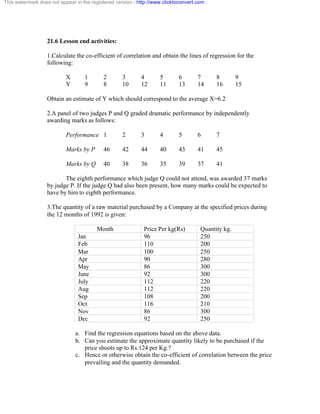
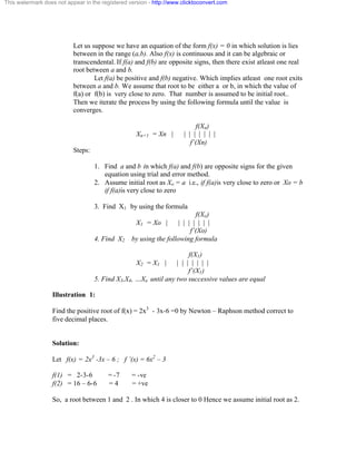
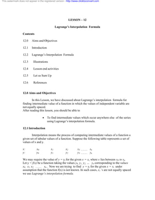
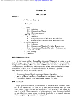
![This watermark does not appear in the registered version - http://www.clicktoconvert.com
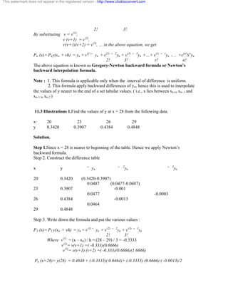
Thus, we continue the iteration and result is noted below
Iteration No. x y z
4 2.40093 3.54513 1.92265
5 2.43155 3.58327 1.92692
6 2.42323 3.57046 1.92565
7 2.42603 3.57395 1.92604
8 2.42527 3.57278 1.92593
9 2.42552 3.57310 1.92596
10 2.42546 3.57300 1.92595
From the above table 9 th and 10 th iterations are equal by considering the four
decimal places. Hence the solution of the equation is
x = 2.4255 y = 3.5730 z =1.9260.
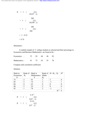
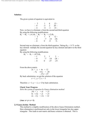
Illustration 2 . Solve the system of equation by Gauss-Jacobi method
10x - 5 y - 2 z = 3
4x - 10y + 3z = -3
x +6y + 10 z = 3
Solution:
To apply this method , first we have to check the diagonal elements are dominant.
i.e., 10 > 5+ 2 ; 10 > 4+ 3 ; 10 > 1+6 . So iteration method can be applied
x = 1/10 (3 + 5 y + 2z )
y =1 /10 (3 + 4x + 3z )
z = 1/10 ( -3 – x - 6y )
First iteration : From the above equations, we start with x = y = z = 0
x(1) = 3/10 = 0 .3 …………….(1)
y(1) = 3/10 = 0 .3 ……………..(2)
z(1) = -3/10 = -0.3 ………………(3)
Second iteration :Consider the new values of y(1) =0 .3 and z(1) = -0.3 in the first
equation
x(2) = 1/10( 3 + 5 x.3 +( -0.3)) = 0.39
y(2) = 1/10 ( 3 + 4 x0 .3 + 3 x( -0.3) ) = 0.33
z(2) = 1/10 [ -3 | (0.3) | 6(0 .3) ] = -0.51
Third iteration : Consider the new values of x(2) = 0.39 , y(2) = 0.33 and z(2)
=-0.51 in the first equation](https://image.slidesharecdn.com/bcanumer-141110101906-conversion-gate02/85/Bca-numer-28-320.jpg)
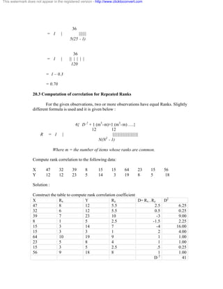
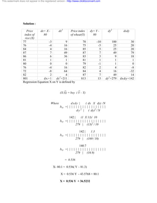
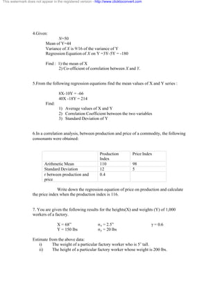
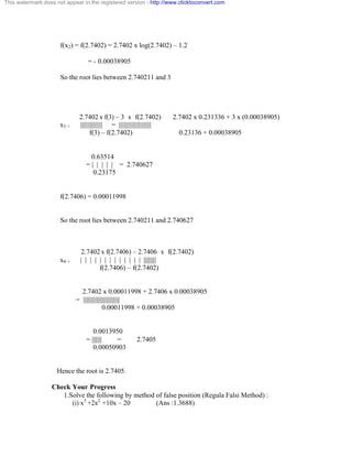
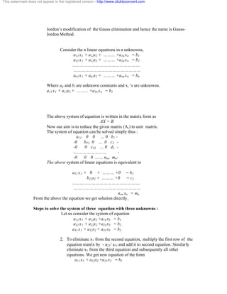
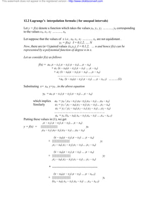
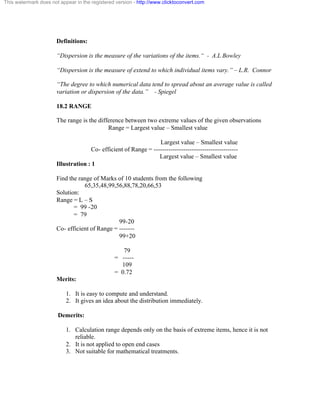
![This watermark does not appear in the registered version - http://www.clicktoconvert.com
x(3) = 1/10 [ 3 | 5 x0.33 +(-0.51)] = 0.363
y(3) = 1/10 ( 3 + 4 x 0.39 + 3 x (-0.51) ) = 0.303
z(3) = 1/10[ -3 | 0.39 | 6 x (0.33) ] = -0.537
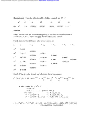
Thus, we continue the iteration and result is noted below
Iteration No. X y z
4 0.3441 0.2841 -0.5181
5 0.33843 0.2822 -0.50487
6 0.340126 0.283911 0.503163
7 0.3413229 0.2851015 -0.5043592
8 0.34167891 0.2852214 -0.50519319
9 0.341572062 0.285113607 -0.505300731
From the above table 8 th and 9 th iterations are equal by considering the 3
decimal places. Hence the solution of the equation is
x =0.342 , y = 0.285, z = - 0.505.
Check Your Progress
1. Solve the system of equation by Gauss-Jacobi method
3.15x – 1.96 y + 3.85 z = 12.95
2.13x - 5.12y -2.892z = -8.61
5.92x +3.051y +2.15 z = 6.88
(Ans : x =1.7089, y = -1.8005, z = 1.0488)
3.4 Lesson End Activities
Solve the following system of equations by using Gauss-Jacobi Method
1. 8x -3y + 2z=20 ; 4x +11y – z = 33; 6x +3y +12 z = 35
2. 28x+4y -z= 32 ; x +3y +10 z = 24; 2x +3y +10 z = 24
3. 5x -2y +z = -4 ; x + 6y -2z = -1; 3x+y+5z = 13
4. 8x +y+z = 8 ; 2x+4y + z = 4 ; x +3y + 3z = 5
3.5 Let us Sum Up
In this lesson we have dealt with the following:
· We have discussed Gauss Jacobi method to solve the system of
linear equations, which occurs in the field of science and
engineering. This method is an iterative method and it is widely
applied.
Model Answer For Lesson End Activities
1. (Ans: 3.017, 1.986, 0.912)
2. (Ans: 0.994, 1.507, 1.849)
3. (Ans:-1.0, .999, 3 )](https://image.slidesharecdn.com/bcanumer-141110101906-conversion-gate02/85/Bca-numer-29-320.jpg)
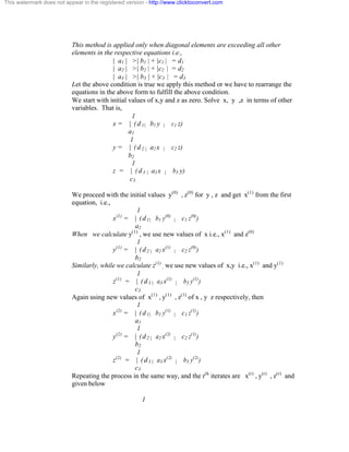
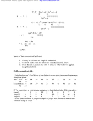
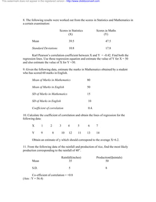
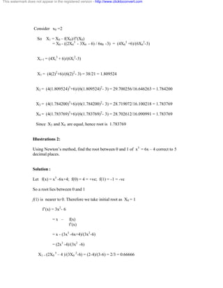
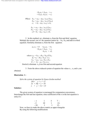
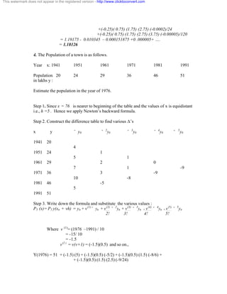
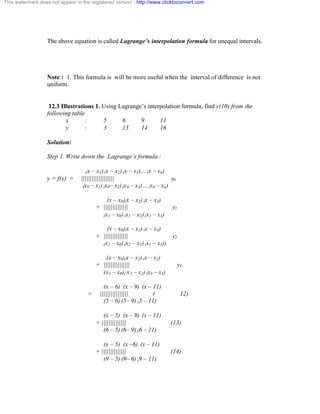
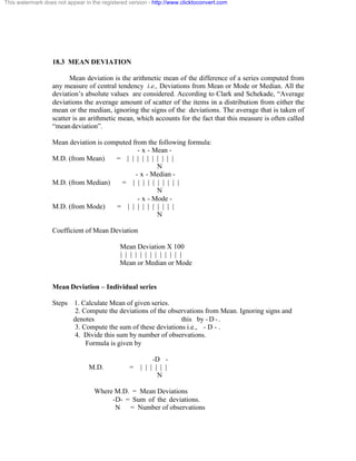
![This watermark does not appear in the registered version - http://www.clicktoconvert.com
x(r+1) = | ( d 1 | b1 y(r) | c1 z(r))
a1
1
y(r+1) = | ( d 2 | a2 x(r+1) | c2 z(r))
b2
1
z(r+1) = | ( d 3 | a3 x(r+1) | b3 y(r+1))
c3
The above iteration is continued until any two successive values are equal.
Note : 1. For all systems of equation, this method will not work
2.Iteration method is self correcting method. Any error made in computation is corrected
automatically in subsequent iterations
3. Iteration is stopped when any two successive iteration values are equal
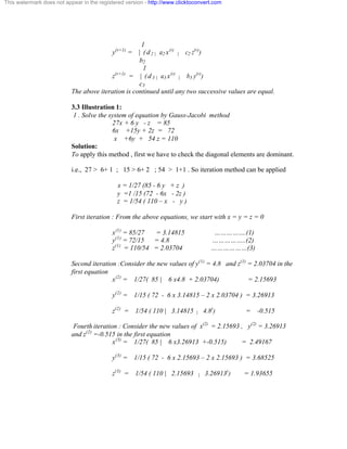
4.3 Illustration : 1 . Solve the system of equation by Gauss-Seidel method
10x - 5 y - 2 z = 3
4x - 10y + 3z = -3
x +6y + 10 z = 3
Solution:
To apply this method , first we have to check the diagonal elements are dominant.
ie., 10 > 5+ 2 ; 10 > 4+ 3 ; 10 > 1+6 . So iteration method can be applied
x = 1/10 (3 + 5 y + 2z )
y =1 /10 (3 + 4x + 3z )
z = 1/10 ( -3 – x - 6y )
First iteration :
From the above equations, we start with x = y = z = 0
x(1) = 3/10 = 0 .3 …………….(1)
New value of x is used for further calculation ie., x = 0.3
y(1) = 1/10 (3 + 4x 0.3+ 3(0)] = 0 .42 ……………..(2)
New values of x and y is used for further calculation ie., x = 0.3 and y = 0.42
z(1) = 1/10 (-3 - 0.3 -6(0.42) = -0.582 ………………(3)
Second iteration :
Consider the new values of y(1) =0 .42 and z(1) = -0.582 in the first equation
x(2) = 1/10( 3 + 5 x 0.42 +( -0.582)) = 0.3936
y(2) = 1/10 ( 3 + 4 x0 .3936 + 3 x( -0.582) ) = 0.28284
z(2) = 1/10 [ -3 | (0.3936) | 6(0 .28284) ] = -0.509064](https://image.slidesharecdn.com/bcanumer-141110101906-conversion-gate02/85/Bca-numer-33-320.jpg)
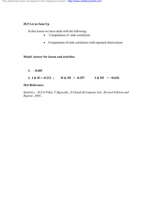
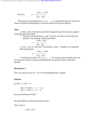
![This watermark does not appear in the registered version - http://www.clicktoconvert.com
Third iteration : Consider the new values of x(2) = 0.3936 , y(2) = 0.28284 and
z(2) =-0.509064 in the first equation
x(3) = 1/10 [ 3 | 5 x0.28284 +(-0.509064)] = 0.3396072
y(3) = 1/10 ( 3 + 4 x 0.3396072 + 3 x (-0.509064 ) = 0.28312368
z(3) = 1/10[ -3 | 0.3396072 | 6 x (0.283123678) ] = -0.503834928
Thus, we continue the iteration and result is noted below
Iteration No. X Y Z
4 0.34079485 0.28516746 -0.50517996
5 0.3415547 0.28506792 -0.505196229
6 0.3414947 0.2850390 -0.5051728
7 0.3414849 0.28504212 -0.5051737
The values correct to 3 decimal places are
x = 0.342, y = 0.285, z = -0.505
Note : Check the above equations by substituting values of x,y and z
Illustration 2 : 1 . Solve the system of equation by Gauss-Seidel method
28x + 4 y - z = 32
4x +3y + 10 z = 24
2x +17y + 4z = 35
Solution:
To apply this method , first we have to rewrite the equation in such way that to
fulfill diagonal elements are dominant.
28x + 4 y - z = 32
2x +17y + 4z = 35
4x +3y + 10 z = 24
ie., 28 > 4+ 1 ; 17 > 2+ 4 ; 10 > 4+3 . So iteration method can be applied
x = 1/28 (32 - 4 y + z )
y =1 /17 (35 -2x -4z )
z = 1/10 ( 24 – x - 3y )
First iteration :
From the above equations, we start with y = z = 0, we get
x(1) = 32/28 = 1.1429
New value of x is used for further calculation ie., x = 1.1429
y(1) = 1/17 (35 + 1.1429+ 3(0)] = 1.9244
New values of x and y is used for further calculation ie., x = 1.1429](https://image.slidesharecdn.com/bcanumer-141110101906-conversion-gate02/85/Bca-numer-34-320.jpg)
![This watermark does not appear in the registered version - http://www.clicktoconvert.com
and y = 1.9244
z(1) = 1/10 [24 -1.1429 -3(1.9244 ) ] = 1.8084)
Second iteration :
Consider the new values of y(1) = 1.9244 and z(1) = 1.8084
x(2) = 1/28[ 32 – 4 (1.9244) +( 1.8084)] = 0.9325
y(2) = 1/17 [ 35 - 2 (0 .9325) - 4 ( 1.8084) ] = 1.5236
z(2) = 1/10 [ 24 | (0.9325) | 3(1.5236) ] = 1.8497
Third iteration :
Consider the new values of x(2 ) = 0.9325, y(2) = 1.5236 and z(2) = 1.8497
x(3) = 1/28[ 32 – 4 (1.5236) +( 1.8497)] = 0.9913
y(3) = 1/17 [ 35 - 2 (0 .9913) - 4 ( 1.8497) ) = 1.5070
z(3) = 1/10 [ 24 | (0.9913) | 3(1.5070) ] = 1.8488
Thus, we continue the iteration and result is noted below
Iteration No. X y Z
4 0.9936 1.5069 1.8486
5 0.9936 1.5069 1.8486
Therefore x = 0.9936, y = 1.5069, z = 1.8486
Check Your Progress
1. Solve the system of equation by Gauss Seidel method
3.15x – 1.96 y + 3.85 z = 12.95
2.13x - 5.12y -2.892z = -8.61
5.92x +3.051y +2.15 z = 6.88
(Ans : x =1.7089, y = -1.8005, z = 1.0488)
4.4 Lesson End Activities
1. 8x -6y +z =13.67; 3x +y -2z =17.59; 2x -6y +9z =29.29
2. 30x – 2y +3z =75; 2x+ 2y +18z = 30 ; x + 17y -2z =48
3. y –x + 10z=35.61; x + z + 10y =20.08; y- z +10x =11.19
4. 10x -2y +z = 12 ; x + 9y -z =10; 2x – y + 11z = 20
5. 8x – y +z =18; 2x +5y -2z = 3; x+y – 3z = -16
6. 2x + y + z =4; x + 2y –z = 4; x + y + 2z = 4](https://image.slidesharecdn.com/bcanumer-141110101906-conversion-gate02/85/Bca-numer-35-320.jpg)
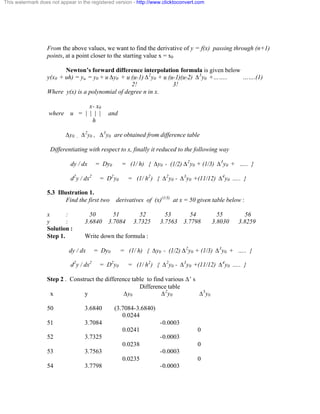
![This watermark does not appear in the registered version - http://www.clicktoconvert.com
0.0232 0
55 3.8030 -0.0003
0.0229
56 3.8259
By applying Newton’s forward formula :
[ dy / dx]x=xo =[ dy / dx]u=o
= (1/ h) { Äy0 - (1/2) Ä2y0 + (1/3) Ä3y0 + ….. }
= (1/ 1) [ 0.0244 - (1/2) (-0.0003) + (1/3) 0 ]
= 0.02455
[d2y / dx2 ]x=50 = D2y0 = (1/ h2) [ Ä2y0 - Ä3y0 +… ]
= 1 [ -0.0003]
= -0.0003
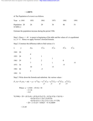
Illustration 2. The population of a certain town is given below. Find the rate of growth
of the population in 1931 and 1941
Year x : 1931 1941 1951 1961 1971
Population y : 40.62 60.80 79.95 103.56 132.65
Solution. Construct the difference table
x y Äy0 Ä2y0 Ä3y0 Ä4y0
1931 40.62
20.18
1941 60.80 -1.03
19.15 5.49
1951 79.95 4.46 -4.47
23.61 1.02
1961 103.56 5.48
29.09
1971 132.65
By applying Newton’s forward formula :
To find (i) f’(1931)
x- x0 1931 - 1931
where u = | | | | = |||||||| = 0](https://image.slidesharecdn.com/bcanumer-141110101906-conversion-gate02/85/Bca-numer-39-320.jpg)
![This watermark does not appear in the registered version - http://www.clicktoconvert.com
h 10
[ dy / dx]x=1931 =[ dy / dx]u=o
= (1/ h) [ Äy0 - (1/2) Ä2y0 + (1/3) Ä3y0 - (1/4) Ä4y0 ]
= (1/ 10) [ 20.18 - (1/2) (-1.03) + (1/3) (5.49) –(-4.47) ]
= (1/ 10) [ 20.18 +0515+1.83+1.1175 ]
= 2.36425
To find (i) f’(1941)
x- x0 1941 - 1931
where u = | | | | = |||||||| = 1
h 10
[ dy / dx]x=1941 =[ dy / dx]u=1
= (1/ h) { Äy0 + [(2u-1)/2] Ä2y0 + [(3u2-6u+2)/6] Ä3y0 +[(4u3 -18u2 +22u-
6)/24 ] Ä4y0 }
= (1/ 10) [ 20.18 + (1/2) (-1.03) –(1/6) (5.49) +(1/12)(-4.47) ]
= (1/ 10) [ 20.18 | 0.515 |0.915|0.3725 ]
= 1.83775
Check Your Progress
4.Find the first two derivatives of t5he function x = 1.5 from the table below
x 1.5 2.0 2.5 3.0 3.5 4.0
y 3.375 7.0 13.625 24.0 38.875 59.0
(Ans : 4.75, 9.0)
5.4 Lesson End Activities
1. Find the first and second derivative of the function tabulated below at x = 3
x : 3.0 3.2 3.4 3.6 3.8 4.0
f(x) : -14 -10.32 -5.296 -0.256 6.672 14
2. Find second derivative of y at x = 0.96 from the data
x : 0.96 0.98 1.00 1.02 1.04
y : 0.7825 0.7739 0.7651 0.7563 0.7473
3. Find the value of cos(1.74) from the following table.](https://image.slidesharecdn.com/bcanumer-141110101906-conversion-gate02/85/Bca-numer-40-320.jpg)
![This watermark does not appear in the registered version - http://www.clicktoconvert.com
54 3.7798 -0.0003
0.0232 0
55 3.8030 -0.0003
0.0229
56 3.8259
By applying Newton’s backward difference formula :
[ dy / dx]x=xn =[ dy / dx]v=o
= (1/ h) { ˘ yn + (1/2) ˘ 2yn + (1/3) ˘ Ä3yn + ….. }
= (1/ 1) [ 0.0299 + (1/2) (-0.0003) + (1/3) 0 ]
= 0.02275
[d2y / dx2 ]x=56 = D2y0 = (1/ h2) [ ˘ 2yn + ˘ 3yn +… ]
= 1 [ -0.0003]
= -0.0003
Illustration 2. The population of a certain town is given below. Find the rate of growth
of the population in 1961 and 1971
Year x : 1931 1941 1951 1961 1971
Population y : 40.62 60.80 79.95 103.56 132.65
Solution. Construct the difference table
x y Äy0 Ä2y0 Ä3y0 Ä4y0
1931 40.62
20.18
1941 60.80 -1.03
19.15 5.49
1951 79.95 4.46 -4.47
23.61 1.02
1961 103.56 5.48
29.09
1971 132.65
By applying Newton’s forward formula :
To find (i) f’(1961)](https://image.slidesharecdn.com/bcanumer-141110101906-conversion-gate02/85/Bca-numer-44-320.jpg)
![This watermark does not appear in the registered version - http://www.clicktoconvert.com
xn- x 1961 - 1971
where v = | | | | = |||||||| = -1
h 10
[ dy / dx]x=1961 =[ dy / dx]v=-1
= (1/ h) { ˘ yn + ((2v+1) / 2) ˘ 2yn + ((3v2+6v+2)/6) ˘ Ä3yn +….. }
= (1/ 10) [29.09 – (1/2) (5.48) – (1/6) (1.02) – (1/12) (-4.47) ]
= (1/ 10) [29.09 – 2.74 -0.17 + 0.3725]
= 2.65525
To find (i) f’(1971)
xn- x 1971 - 1971
where v = | | | | = | | | | | | | | = 0
h 10
[ dy / dx]x=1971 =[ dy / dx]v=0
= (1/ h) { ˘ yn + (1 / 2) ˘ 2yn + (1/3) ˘ Ä3yn +(1/4) ˘ Ä4yn ….. }
= (1/ 10) [29.09 + (1/2) (5.48) + (1/3) (1.02) + (1/4) (-4.47) ]
= (1/ 10) [29.09 + 2.74 +0.34 - 1.1175]
= 2.65525
6.4 Lesson End Activities
1. find the first and second derivative of the function tabulated below at x = 4.0
x : 3.0 3.2 3.4 3.6 3.8 4.0
f(x) : -14 -10.32 -5.296 -0.256 6.672 14
2. find second derivative of y at x = 1.04 from the data
x : 0.96 0.98 1.00 1.02 1.04
y : 0.7825 0.7739 0.7651 0.7563 0.7473
3. From the table below find y’ and y’’ at x = 1.25
x : 1.00 1.05 1.10 1.15 1.20 1.25 1.30
y : 1.00000 1.02470 1.04881 1.07238 1.09544 1.11803 1.14017](https://image.slidesharecdn.com/bcanumer-141110101906-conversion-gate02/85/Bca-numer-45-320.jpg)
![This watermark does not appear in the registered version - http://www.clicktoconvert.com
From the above values, we want to find the integration of y = f(x) with the range x0 and
x0 +mh
xo x0+mh f(x) dx = (h/2) [ (y0 + yn) + 2 (y1 + y2+ y3+ …. + yn-1) ]
= (h/2) [ (sum of the first and last ordinates ) +
(Sum of the remaining ordinates) ]
7.3 Illustrations 1. Evaluate -3 3 x4 dx by using Trapezoidal rule. Verify result by
actual integration.
Step 1. We are given that f(x) = x4. Interval length (b –a ) = (3 – (-3) ) = 6. So we
divide 6 equal intervals with h= 6/6 = 1.0 And tabulate the values as below
x : -3 -2 -1 0 1 2 3
y : 81 16 1 0 1 16 81
Step2. Write down the trapezoidal rule and put the respective values in that rule
-3 3 f(x) dx = (h/2) [ (y0 + yn) + 2 (y1 + y2+ y3+ …. + yn-1) ]
= (h/2) [ (sum of the first and last ordinates ) +
(Sum of the remaining ordinates) ]
= (1/2) [ (81+81) + 2 (16+1+0+1+16) ]
= 115
By actual integration -3 3 f(x) dx = -3 3 x4 dx
= [ (35/5) -(-35/5) ]
=[ (243/5) + (243/5)]
= 97.5
Illustration 2 :Evaluate 0 1 1/(1+x2) dx by using Trapezoidal rule with h = 0.2
Solution:
Step 1. We are given that f(x) = 1/(1+x2). Interval length (b –a ) = (1 – 0 ) = 1. So we
divide 6 equal intervals with h= 0.2 And tabulate the values as below
x : 0 0.2 0.4 0.6 0.8 1.0
y1/(1+x2): 1 0.96154 0.86207 0.73529 0.60976 0.5000
Step2. Write down the trapezoidal rule and put the respective values of y in that rule](https://image.slidesharecdn.com/bcanumer-141110101906-conversion-gate02/85/Bca-numer-48-320.jpg)
![This watermark does not appear in the registered version - http://www.clicktoconvert.com
-3 3 f(x) dx = (h/2) [ (y0 + yn) + 2 (y1 + y2+ y3+ …. + yn-1) ]
= (h/2) [ (sum of the first and last ordinates ) +
(Sum of the remaining ordinates) ]
= (0.2/2) [ (1+0.5) + 2 (0.96154+0.86207+0.73529+0.60976) ]
= (0.1) [ (1.05) + 6.33732 ]
= 0.783732
Illustration 3. Evaluate 0 6 1/ (1+x) dx by using Trapezoidal rule .
Solution:
Step 1. We are given that f(x) = 1/(1+x). Interval length (b –a ) = (6 – 0 ) = 6. So we
divide 6 equal intervals with h= 1. And tabulate the values as below
x : 0 1 2 3 4 5 6
y1/(1+x2): 1 0.5 1/3 1/4 1/5 1/6 1/7
Step2. Write down the trapezoidal rule and put the respective values of y in that rule
-3 3 f(x) dx = (h/2) [ (y0 + yn) + 2 (y1 + y2+ y3+ …. + yn-1) ]
= (h/2) [ (sum of the first and last ordinates ) +
(Sum of the remaining ordinates) ]
= (1/2) [ (1+1/7) + 2 (0.5+1/3 + 1/4 + 1/5 +1/6 ) ]
= (0.5) [ (1.05) + 6.33732 ]
Illustration 4. Evaluate 4 5.2 loge x dx by using Trapezoidal rule .
Solution:
Step 1. We are given that f(x) = loge x Interval length (b –a ) = (5.2 – 4 ) = 1.2. So we
divide 6 equal intervals with h= 0.2. And tabulate the values as below
x : 4 4.2 4.4 4.6 4.8 5.0 5.2
y : 1.39 1.44 1.48 1.53 1.57 1.61 1.65](https://image.slidesharecdn.com/bcanumer-141110101906-conversion-gate02/85/Bca-numer-49-320.jpg)
![This watermark does not appear in the registered version - http://www.clicktoconvert.com
Step2. Write down the trapezoidal rule and put the respective values of y in that rule
-3 3 f(x) dx = (h/2) [ (y0 + yn) + 2 (y1 + y2+ y3+ …. + yn-1) ]
= (h/2) [ (sum of the first and last ordinates ) +
(Sum of the remaining ordinates) ]
= (0.2/2) [ (1.39+1.65) + 2 (1.44 +1.48 + 1.53+ 1.57 +1.61) ]
= (0.1) [ 3.04 + 2(7.63) ]
= 1.83
Illustration 5. Evaluate 0 ð sin x dx by using Trapezoidal rule, by dividing the range
into ten equal parts .
Solution :
Step 1. We are given that f(x) = sin x Interval length (b –a ) = (ð – 0 ) =ð.
So we divide 10 equal intervals with h= ð/10 (specified in the question itself),
and tabulate the values as below
x: 0 ð/10 2ð/10 3ð/10 4ð/10
Y: 0.0 0.3090 0.5878 0.8090 0.9511
x: 5ð/10 6ð/10 7ð/10 8ð/10 9ð/10 ð
Y: 1.0 0.9511 0.8090 0.5878 0.3090 0
Step2. Write down the trapezoidal rule and put the respective values of y in that rule
-3 3 f(x) dx = (h/2) [ (y0 + yn) + 2 (y1 + y2+ y3+ …. + yn-1) ]
= (h/2) [ (sum of the first and last ordinates ) +
(Sum of the remaining ordinates) ]
=(ð/20)[(0+0)+2(0.3090+0.5878+0.8090+0.9511+1.0+
0.9511+0.8090+0.5878+0.309)]
= 1.9843](https://image.slidesharecdn.com/bcanumer-141110101906-conversion-gate02/85/Bca-numer-50-320.jpg)
![This watermark does not appear in the registered version - http://www.clicktoconvert.com
7.3 Simpson’s one third Rule
Suppose the following table represents a set of values of x and y.
x: x0 x1 x2 x3 ……….. xn
y: y0 y1 y2 y3 ……….. yn
From the above values, we want to find the integration of y = f(x) with the range x0 and
x0 + nh
xo xn f(x) dx = (h/3) [ (y0 + yn) + 2 (y2 + y4 + ) + 4 (y1+ y3+ …. ) ]
= (h/3) [ (sum of the first and last ordinates ) +
+ 2 (Sum of remaining even ordinates)
+4 ( sum of remaining odd ordinates)]
The above equation is called Simpson’s one third rule and it is applicable only when
number of ordinates must be odd ( no. of pairs ).
8.3 Illustrations 1. Evaluate -3 3 x4 dx by using Simpson’s one third rule. Verify result
by actual integration.
Step 1. We are given that f(x) = x4. Interval length (b –a ) = (3 – (-3) ) = 6. So we
divide 6 equal intervals with h= 6/6 = 1.0 And tabulate the values as below
x : -3 -2 -1 0 1 2 3
y : 81 16 1 0 1 16 81
Step2. Write down the Simpson’s one third rule and put the respective values in that rule
-3 3 f(x) dx ) = (h/3) [ (y0 + y6) + 2 (y2 + y4 ) + 4 (y1+ y3+y5 ) ]
= (h/3) [ (sum of the first and last ordinates ) +
+ 2 (Sum of remaining even ordinates)
+4 ( sum of remaining odd ordinates) ]
= (1/3) [ (81+81) + 2 (1+1) +4(16+1+16) ]
= 98
By actual integration -3 3 f(x) dx = -3 3 x4 dx
= [ (35/5) -(-35/5) ]
=[ (243/5) + (243/5)]
= 97.5](https://image.slidesharecdn.com/bcanumer-141110101906-conversion-gate02/85/Bca-numer-53-320.jpg)
![This watermark does not appear in the registered version - http://www.clicktoconvert.com
2. Evaluate 0 1.2 1/(1+x2) dx by using Simpson’s one third rule with h = 0.2
Solution:
Step 1. We are given that f(x) = 1/(1+x2). Interval length (b –a ) = (1.2 – 0 ) = 1.2 . So
we divide 6 equal intervals with h= 0.2 And tabulate the values as below
x : 0 0.2 0.4 0.6 0.8 1.0 1.2
y1/(1+x2): 1 0.9615 0.8621 0.7353 0.6098 0.5000 0.4098
Step2. Write down the Simpson’s one third rule and put the respective values of y in that
rule
-3 3 f(x) dx = (h/3) [ (y0 + y6) + 2 (y2 + y4 ) + 4 (y1+ y3+y5 ) ]
= (h/3) [ (sum of the first and last ordinates ) +
+ 2 (Sum of remaining even ordinates)
+4 ( sum of remaining odd ordinates) ]
= (0.2 /3) [ (1+0.4098) + 2 (0.8621 +0.6098) + 4 (0.9615+0.7353+0.5 ) ]
= (0.0667) [ (1.4098) +2(1.4719) + 4 (2.1503) ]
= (0.0667) [ 1.4098 + 2.9438 + 8.6012]
=0.8641
3. Evaluate 0 6 1/ (1+x) dx by using Simpson’s one third rule .
Solution:
Step 1. We are given that f(x) = 1/(1+x). Interval length (b –a ) = (6 – 0 ) = 6. So we
divide 6 equal intervals with h= 1. And tabulate the values as below
x : 0 1 2 3 4 5 6
y1/(1+x2): 1 0.5 1/3 1/4 1/5 1/6 1/7
Step2. Write down the Simpson’s one third rule and put the respective values of y in that
rule](https://image.slidesharecdn.com/bcanumer-141110101906-conversion-gate02/85/Bca-numer-54-320.jpg)
![This watermark does not appear in the registered version - http://www.clicktoconvert.com
-3 3 f(x) dx = (h/3) [ (y0 + y6) + 2 (y2 + y4 ) + 4 (y1+ y3+y5 ) ]
= (h/3) [ (sum of the first and last ordinates ) +
+ 2 (Sum of remaining even ordinates)
+4 ( sum of remaining odd ordinates) ]
= (1/3) [ (1+1/7) + 2 (1/3 + 1/5) + 4( 0.5 +1/4 +1/6 ) ]
= 1.9587
4. Evaluate 4 5.2 loge x dx by using Simpson’s one third rule .
Solution:
Step 1. We are given that f(x) = loge x Interval length (b –a ) = (5.2 – 4 ) = 1.2. So we
divide 6 equal intervals with h= 0.2. And tabulate the values as below
x : 4 4.2 4.4 4.6 4.8 5.0 5.2
y : 1.39 1.44 1.48 1.53 1.57 1.61 1.65
Step2. Write down the Simpson’s one third rule and put the respective values of y in that
rule
-3 3 f(x) dx = (h/3) [ (y0 + y6) + 2 (y2 + y4 ) + 4 (y1+ y3+y5 ) ]
= (h/3) [ (sum of the first and last ordinates ) +
+ 2 (Sum of remaining even ordinates)
+4 ( sum of remaining odd ordinates) ]
= (0.2/3) [ (1.39+1.65) + 2 (1.48+ 1.57) + 4 (1.44+ 1.53++1.61) ]
= (0.0667) [ 3.04 + 2(3.05)+ 4 (4.58) ]
= 1.83
5. Evaluate 0 ð sin x dx by using Simpson’s one third rule, by dividing the range into
ten equal parts .
Solution :](https://image.slidesharecdn.com/bcanumer-141110101906-conversion-gate02/85/Bca-numer-55-320.jpg)
![This watermark does not appear in the registered version - http://www.clicktoconvert.com
Step 1. We are given that f(x) = sin x Interval length (b –a ) = (ð – 0 ) =ð.
So we divide 10 equal intervals with h= ð/10 (specified in the question itself),
and tabulate the values as below
x: 0 ð/10 2ð/10 3ð/10 4ð/10
Y: 0.0 0.3090 0.5878 0.8090 0.9511
x: 5ð/10 6ð/10 7ð/10 8ð/10 9ð/10 ð
Y: 1.0 0.9511 0.8090 0.5878 0.3090 0
Step2. Write down the Simpson’s one third rule and put the respective values of y in that
rule
-3 3 f(x) dx =(h/3) [ (y0 + y10) + 2 (y2 + y4 + y6 + y8 ) + 4 (y1+ y3+y5+ y7 + y9 ) ]
= (h/3) [ (sum of the first and last ordinates ) +
+ 2 (Sum of remaining even ordinates)
+4 ( sum of remaining odd ordinates
=(ð/20)[(0+0)+2(0.5878+ 0.9511+0.9511+0.5878) +
4(0.3090+0.8090+ 1+ 0.8090+0.3090)]
= 2.0009
8.4 Lesson End Activities
2. Evaluate 1 2 1/(1+x2) dx taking h = 0.2 using Simpson’s one third rule.
2. Compute the value of 1 2 dx/ x using Simpson’s one third rule. Take h 0.25
3. Evaluate 0 ð/2 sin x dx by using Simpson’s one third rule, by dividing the range
into ten equal parts .)
____________
4. Evaluate 0 1 sin x + cos x dx by using Simpson’s one third rule, by dividing the
range into seven equal parts .
8.5 Let us Sum Up
In this lesson we have dealt with the following:
We have discussed about the Simpson’s one third rule to evaluate
integration. This method more easier than any other method.](https://image.slidesharecdn.com/bcanumer-141110101906-conversion-gate02/85/Bca-numer-56-320.jpg)
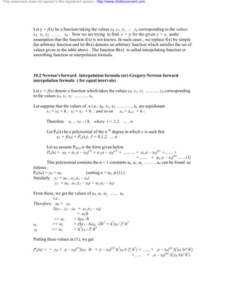
![This watermark does not appear in the registered version - http://www.clicktoconvert.com
9.2 Simpson’s three-eighth Rule
Suppose the following table represents a set of values of x and y.
x: x0 x1 x2 x3 ……….. xn
y: y0 y1 y2 y3 ……….. yn
From the above values, we want to find the integration of y = f(x) with the range x0 and
x0 +h
xo xn f(x) dx = (3h/8 ) [ (y0 + yn) + 2 (y3 + y6+ y9 +… ) + 3 (y1 + y2 + y4 + y5 + …….+yn-1 )]
= (3h/8) [ (sum of the first and last ordinates ) +
+ 2 (Sum of multiples of three ordinates)
+3 ( sum of remaining ordinates)]
The above equation is called Simpson’s three-eighths rule which is applicable only when
n is multiple of 3 .
9.3 Illustrations 1. Evaluate -3 3 x4 dx by using Simpson’s three-eighth rule. Verify
result by actual integration.
Step 1. We are given that f(x) = x4. Interval length (b –a ) = (3 – (-3) ) = 6. So we
divide 6 equal intervals with h= 6/6 = 1.0 And tabulate the values as below
x : -3 -2 -1 0 1 2 3
y : 81 16 1 0 1 16 81
Step2. Write down the Simpson’s three-eighth rule and put the respective values in that
rule
-3 3 f(x) dx ) = (3h/8) [ (y0 + y6) + 2 (y3 ) + 3 (y1 + y2+ y4+ y5 ) ]
= (3h/8) [ (sum of the first and last ordinates ) +
+ 2 (Sum of multiples of three, other than last ordinates )
+3 ( sum of remaining ordinates)]
= (3/8) [ (81+81) + 2 (0)) + 3(16+1+1+16) ]
= 99
By actual integration -3 3 f(x) dx = -3 3 x4 dx
= [ (35/5) -(-35/5) ]](https://image.slidesharecdn.com/bcanumer-141110101906-conversion-gate02/85/Bca-numer-59-320.jpg)
![This watermark does not appear in the registered version - http://www.clicktoconvert.com
=[ (243/5) + (243/5)]
= 97.5
6. Evaluate 0 1.2 1/(1+x2) dx by using Simpson’s three-eighth rule with h = 0.2
Solution:
Step 1. We are given that f(x) = 1/(1+x2). Interval length (b –a ) = (1 – 0 ) = 1. So we
divide 6 equal intervals with h= 0.2 and tabulate the values as below
x : 0 0.2 0.4 0.6 0.8 1.0 1.2
y1/(1+x2): 1 0.9615 0.8621 0.7353 0.6098 0.5000 0.4098
Step2. Write down the Simpson’s three-eighth rule and put the respective values of y in
that rule
-3 3 f(x) dx = (3h/8) [ (y0 + y6) + 2 (y3 ) + 3 (y1 + y2+ y4+ y5 ) ]
= (3h/8) [ (sum of the first and last ordinates ) +
+ 2 (Sum of multiples of three, other than last ordinates )
+3 ( sum of remaining ordinates) ]
= (3 x 0.2 /3) [ (1+0.4098) + 2 (0.7353 )
+ 3 (0.9615+0.8621+0.6098 + 0.5 ) ]
= (0.075) [1.4098 + 1.4706 + 3 ( 2.9334) ]
= (0.075) [ 1.4098 + 1.4706 + 8.8002]
=0.8760
7. Evaluate 0 6 1/ (1+x) dx by using Simpson’s three-eighth rule .
Solution:
Step 1. We are given that f(x) = 1/(1+x). Interval length (b –a ) = (6 – 0 ) = 6. So we
divide 6 equal intervals with h= 1. And tabulate the values as below
X : 0 1 2 3 4 5 6
y = 1/(1+x2)x : 1 0.5 1/3 1/4 1/5 1/6 1/7
Step2. Write down the Simpson’s three-eighth rule and put the respective values of y in
that rule](https://image.slidesharecdn.com/bcanumer-141110101906-conversion-gate02/85/Bca-numer-60-320.jpg)
![This watermark does not appear in the registered version - http://www.clicktoconvert.com
-3 3 f(x) dx = (3h/8) [ (y0 + y6) + 2 (y3 ) + 3 (y1 + y2+ y4+ y5 ) ]
= (3h/8) [ (sum of the first and last ordinates ) +
+ 2 (Sum of multiples of three, other than last ordinates )
+3 ( sum of remaining ordinates )]
= (3/8) [ (1+1/7) + 2 (1/4) + 3 ( 0.5 + 1/3 + 1/5 +1/6 ) ]
= 1.9661
8. Evaluate 4 5.2 loge x dx by using Simpson’s three-eighth rule .
Solution:
Step 1. We are given that f(x) = loge x Interval length (b –a ) = (5.2 – 4 ) = 1.2. So we
divide 6 equal intervals with h= 0.2. And tabulate the values as below
x : 4 4.2 4.4 4.6 4.8 5.0 5.2
y : 1.39 1.44 1.48 1.53 1.57 1.61 1.65
Step2. Write down the Simpson’s three-eighth rule and put the respective values of y in
that rule
-3 3 f(x) dx = (3h/8) [ (y0 + y6) + 2 (y3 ) + 3 (y1 + y2+ y4+ y5 ) ]
= (3h/8) [ (sum of the first and last ordinates ) +
+ 2 (Sum of multiples of three, other than last ordinates )
+3 ( sum of remaining ordinates ) ]
= (3x 0.2 /8 ) [ (1.39+1.65) + 2 (1.53) + 3 (1.44+ 1.48 +1.57++1.61) ]
= (0.075 ) [ 3.04 + 3.06 + 3 (6.1) ]
= 1.83
9. Evaluate 0 9 x2 dx by using Simpson’s three-eighth rule, by dividing the range into
nine equal parts and verify your answer with actual integration.
Solution :
Step 1. We are given that f(x) = x2 Interval length (b –a ) = (9 – 0 ) =9.](https://image.slidesharecdn.com/bcanumer-141110101906-conversion-gate02/85/Bca-numer-61-320.jpg)
![This watermark does not appear in the registered version - http://www.clicktoconvert.com
So, we divide 9 equal intervals with h=9 /9 = 1 (specified in the question itself),
and tabulate the values as below
X : 0 1 2 3 4
Y = x2:0 1 4 9 16
x: 5 6 7 8 9
Y: 25 36 49 64 81
Step2. Write down the Simpson’s three-eighth rule and put the respective values of y in
that rule
-3 3 f(x) dx = (3h/8) [ (y0 + y9) + 2 (y3 + y6 ) + 3 (y1 + y2+ y4+ y5+ y7+ y8 ) ]
= (3h/8) [ (sum of the first and last ordinates ) +
+ 2 (Sum of multiples of three, other than last ordinates )
+3 ( sum of remaining ordinates ) ]
= (3/8) [ (0 +81) + 2 ( 9 + 36) + 3 ( 1+ 4 + 16 + 25 + 49 + 64 ) ]
= (.375) [ 81 + 90 + 477 ]
= 243
By actual integration 0 9 f(x) dx = 0 9 x2 dx
= [ (93/3) -( 03/3) ]
=[ (729 / 3) + 0]
= 243
9.4 Lesson End Activities
1. Evaluate 1 2.2 1/(1+x2) dx taking h = 0.2 using Simpson’s three eighth rule.
2. Compute the value of 0 1.2 dx/ x using Simpson’s three eighth rule. Take h = 0.2
3. Evaluate 0 ð/2 sin x dx by using Simpson’s three eighth rule, by dividing the range
into nine equal parts .
4. Evaluate 0 6 sin x + cos x dx by using Simpson’s three eighth rule, by dividing
the range into six equal parts .](https://image.slidesharecdn.com/bcanumer-141110101906-conversion-gate02/85/Bca-numer-62-320.jpg)
![This watermark does not appear in the registered version - http://www.clicktoconvert.com
Where u(1) = (x – x0) / h = (21 – 20) / 3 = 0.3333
u(2) = u(u-1) = (0.3333)(0.6666)
Pn (x=21)= y(21) = 0.3420 + (0.3333)( 0.0487)+ (0.3333) (-0.6666) ( -0.001)
+ (0.3333) (-0.6666)(-1.6666) ( -0.0003)
= 0.3583
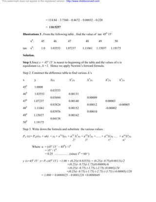
Illustrations 2 . From the following table of half yearly premium for policies maturing at
different ages, estimate the premium for policies maturing at age 46.
Age x: 45 50 55 60 65
Premium y: 114.84 96.16 83.32 74.48 68.48
Solution.
Step 1.Since x = 46 is nearer to beginning of the table and the values of x is equidistant
i.e., h = 5.. Hence we apply Newton’s forward formula.
Step 2. Construct the difference table
x y Äy0 Ä2y0 Ä3y0 Ä4y0
45 114.84
-18.68
50 96.16 5.84
-12.84 -1.84
55 83.12 4.00 0.68
-8.84 -1.16
60 74.48 2.84
-6.00
65 68.48
Step 3. Write down the formula and put the various values :
Pn (x)= Pny(x0 + uh) = y0 + u(1)Äy0 + u(2) Ä2y0 + u(3)Ä3y0 +……+ u(r)Äry0 +.... + u(n)Äny0
2! 3! r! n!
Where u = (x – x0) / h = (46 – 45) / 5 = 01/5 = 0.2
Pn (x=46)= y(46) = 114.84 + [0.2 (-18.68)] +[0.2 (-0.8) (5.84)/ 3]
+ [0.2 (-0.8) (-1.8)(-1.84)/6 ]
+ [0.2 (-0.8) (-1.8)(-2.8)(0.68)]](https://image.slidesharecdn.com/bcanumer-141110101906-conversion-gate02/85/Bca-numer-67-320.jpg)

![This watermark does not appear in the registered version - http://www.clicktoconvert.com
+(-0.3333) (0.6666)(1.6666) ( -0.0003)/6
= 0.4848 – 0.015465 +0.0001444 + 0.0000185
= 0.4695
Illustrations 2 . From the following table of half yearly premium for policies maturing at
different ages, estimate the premium for policies maturing at age 63.
Age x: 45 50 55 60 65
Premium y: 114.84 96.16 83.32 74.48 68.48
Solution.
Step 1.Since x = 63 is nearer to beginning of the table and the values of x is equidistant
i.e., h = 5.. Hence we apply Newton’s backward formula.
Step 2. Construct the difference table
x y ˘ y0 ˘ 2y0 ˘ 3y0 ˘ 4y0
45 114.84
-18.68
50 96.16 5.84
-12.84 -1.84
55 83.12 4.00 0.68
-8.84 -1.16
60 74.48 2.84
-6.00
65 68.48
Step 3. Write down the formula and put the various values :
P3 (x)= P3 y(xn + vh) = yn + v(1)˘ yn + v(2) ˘ 2yn + v(3) ˘ 3yn + v(4) ˘ 4yn
2! 3! 4!
Where v(1) = (x – xn) / h = (63 – 65) / 5 = -2/5 = - 0.4
v(2) = v(v+1) = ( -0.4)(1.6)
v(3) = v(v+1) (v+2) = ( -0.4)(1.6) (2.6)
v(4) = v(v+1) (v+2) ) (v+3) = ( -0.4)(1.6) (2.6)(3.6)
P4 (x=63)= y(63) = 68.48 + [(-0.4) (-6.0)] +[(-0.4) (1.6) (2.84)/ 2]
+ [(-0.4) (1.6) (2.6)(-1.16)/6 ]
+ [(-0.4) (1.6) (2.6)(3.6) (0.68)/24 ]
= 68.48 +2.40 - 0.3408 +0.07424 – 0.028288
= 70.5852](https://image.slidesharecdn.com/bcanumer-141110101906-conversion-gate02/85/Bca-numer-74-320.jpg)
![This watermark does not appear in the registered version - http://www.clicktoconvert.com
y2, y3,….. yn. Computation of these approximate values is known as numerical solution of
the differential equation. Many techniques are available for the approximate solution of
ordinary differential equations by numerical methods. In this lesson we consider the most
frequently used Taylor Method
13.2 Taylor Method
Suppose we want to find the numerical solution of the equation
dy:
| = f(x,y)
dx
Given the initial condition y(x0) = y0
y(x) can be expanded about the point x = x0 in a Taylor’s series as
Suppose the following table represents a set of values of x and y.
x: x0 x1 x2 x3 ……….. xn
y: y0 y1 y2 y3 ……….. yn
From the above values, we want to find the derivative of y = f(x), passing through (n+1)
points, at a point closer to the starting value x = x0
y(x) = y(x0) + (x – x0)1 [ y’(x)]xo /1! + (x – x0)2 [y’’(x) ] xo / 2! + ...
y(x) = y0 + (x – x0)1 y’0 /1! + (x – x0)2 y0’’ / 2! + ...
Putting x = x1 = x0+h, we get
y1 = y0 + h y’0 /1! + h2 y0’’ / 2! + h3 y0’’’ / 3! + ...
Now y(x) can be expanded about the point x = x1 in a Taylor’s series as
y2 = y1+ h y’1 /1! + h2 y1’’ / 2! + h3 y1’’’ / 3! + ...
Proceeding in the same way, we get
yn+1 = yn+ h y’n /1! + h2 yn’’ / 2! + h3 yn’’’ / 3! + ...
In the above equation yr
n = [ dry/dxr](xn,yn) and also an infinite series and hence we have
to truncate at some term to have the numerical value calculated.
For calculation purpose, the terms unto and including hn and neglect terms involving
hn+1, the Taylor algorithm used is said to be of nth order. By increasing the number of
terms in the series, the error can be reduced further .
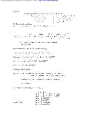
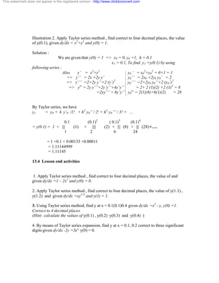
13.3 Illustrations 1. Solve dy/dx = x +y , given y(1) = 0, and get y(1.1) , y(1.2) by
Taylor series method. Compare the result with the actual solution.](https://image.slidesharecdn.com/bcanumer-141110101906-conversion-gate02/85/Bca-numer-86-320.jpg)
![This watermark does not appear in the registered version - http://www.clicktoconvert.com
Improved Euler method
Slight change may be included in the above mentioned algorithm ., i.e., we approximate
the curve by the tangent and we get improved Euler formula ;
yn+1 = yn +(1/2) h[ f(xn,yn)+ f(xn+h, yn+h f(xn,yn) )
This equation is called improved Euler’s method.
Modified Euler method
Slight change may be included in the above mentioned improved Euler’s method., i.e.,
we averaged the slopes, whereas in modified Euler method, we will average the points.
We get the formula for Modified Euler method , given by
yn+1 = yn + h[ f(xn+h/2, yn+(h/2) f(xn,yn) ]
or y(x+h) = y(x) + h[ f(x+h/2, y+(h/2) f(x,y) ]
This equation is called Modified Euler’s method.
Note : 1. Use the formula correctly, after understanding the problem.
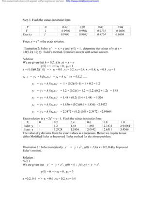
14.4 Illustration 1: Solve y’ = - y ,and y(0) = 1, determine the values of y at x =
(0.01)(0.01)(0.04) by Euler’s method.
Solution.
Step 1.
Calculate various values of xi
‘ s and respective yi’s
We are given that y’ = -y and y(0) = 1 ; f(x,y) = -y;
x = (0.01)(0.01)(0.04) = > x0 = 0, y0 = 1
x1 = 0.01, x1 = 0.01, x2 = 0.02, x3 = 0.03, x4 = 0.04
Step 2. To find y1, y2, y3, y4. Take h = 0.01 (Specified in the problem itself)
Write down the Euler formula ,
yn+1 = yn + h f(xn,yn) = yn + h yn’ ; n = 0,1,2, …..
y1 = y0 + h f(x0,y0) = 1 + (0.01) (-1) = 1 – 0.01 = 0.99
y2 = y1 + h f(x1,y1) = 0.99 + (0.01) (- y1) = 0.99 + (0.01) (- 0.99) = 0.9801
y3 = y2 + h f(x2,y2) = 0.9801 + (0.01) (- 0.9801) = 0.9703
y4 = y3 + h f(x3,y3) = 0.9703 + (0.01) (- 0.9703) =x 0.9606](https://image.slidesharecdn.com/bcanumer-141110101906-conversion-gate02/85/Bca-numer-92-320.jpg)
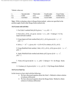
![This watermark does not appear in the registered version - http://www.clicktoconvert.com
Step 2. Write down the formula for Improved Euler method
yn+1 = yn +(1/2) h[ f(xn,yn)+ f(xn+h, yn+h f(xn,yn) ]
y1 = y0 + (1/2) h[ f(x0,y0)+ f(x0+h, y0+h f(x0,y0) ) ) ]
= 0 + (0.5) (0.2) [ y0 + exo + y0 + h(y0 + exo) + exo+h ]
= 0.1 [0+1+0+0.2(0+1)+e0.2]
= 0.1 (1 +0.2 +1.2214)
ð y(0.2) = 0.24214
y2 = y1 + (1/2) h[ f(x1,y1)+ f( x1+h, y1+h f(x1,y1) ) ) ]
where f(x1,y1) = y1 + ex1 =0.24214 + e 0.2 = 1.46354
y1+h f(x1,y1) = 0.24214 + (0.2)(1.46354) = 0.53485
f( x1+h, y1+h f(x1,y1) = f(0.4, 0.53485) = 0.53485 + e0.4 = 2.02667
Substituting the above values, we get
y(0.4) = 0.24212+(0.5)(0.2)[1.46354+2.02667]
= 0.59116
Tabulate the values and it given below:
x 0 .0.2 0.4
y 0 0.24214 0.59116
Illustration 4. Compute y at x = 0.25 by Modified Euler method given y’ = 2xy,
y(0) = 1.
Solution :
Step 1.
We are given that f(x,y) = 2xy ;
y(0) = > x0 = 0, y0 = 1
h = 0.25 => x1 = 0+ 0.25 = 0.25
Step 2. Write down the Modified Euler formula
yn+1 = yn + h[ f(xn+h/2, yn+(h/2) f(xn,yn)]
=> y1 = y0 + h[ f(x0+h/2, y0+(h/2) f(x0,y0) ]
= 1 + (0.25)[f(0.125,1]
= 1 + (0.25)[2 x (0.125) x 1]
= 1.0625.](https://image.slidesharecdn.com/bcanumer-141110101906-conversion-gate02/85/Bca-numer-94-320.jpg)
![This watermark does not appear in the registered version - http://www.clicktoconvert.com
Note : By solving the equation y(0.25) = 1.0645 and error is only 0.002 To
improve the result take h= 0.125 iterate twice, which incurs lot of mathematical
calculation.
14.3 Runge-Kutta Method
Suppose we want to find the numerical solution of the equation
dy
| = f(x,y)
dx
Given the initial condition y(x0) = y0. ……………….(1)
Calculate
k1 = h f(x0 , yo)
k2 = h f(x0 +(1/2)h, yo+(1/2)k1)
and Äy == k2, where h = Äx
The above mentioned algorithm is Second order Runge-Kutta Algorithm
Calculate
k1 = h f(x0 , yo)
k2 = h f(x0 +(1/2)h, yo+(1/2)k1)
k3 = h f(x0 +(1/2)h, yo+(1/2)k2)
and Äy = (1/6)[k1+ 4k2+ k3)
The above mentioned algorithm is Third order Runge-Kutta Algorithm
Calculate
k1 = h f(x0 , yo)
k2 = h f(x0 +(1/2)h, yo+(1/2)k1)
k3 = h f(x0 +(1/2)h, yo+(1/2)k2)
k4 = h f(x0+h , yo +k3)
and Äy = (1/6)[k1+ 2k2+2 k3+ k4]
y(x+h) = y(x) +Äy
The above mentioned algorithm is Fourth order Runge-Kutta Algorithm
Where Äx = h.
Calculate
y1 = y0 + Äy
Now starting from (x1,y1) and repeating the above process, we get (x2,y2) etc.
Note 1: In second order Runge–Kutta method
Äy0 = k2 = h f(x0 +(1/2)h, yo+(1/2)k1)
Äy0 = k2 = h f(x0 +(1/2)h, yo+(1/2)h f(x0,y0)) )
Therefore
y1 = y0 + h[ f(x0+h/2, y0+(h/2) f(x0,y0) ]
This is equivalent to modified Euler Method.
Hence, the Runge-Kutta method of second order is nothing but the Modified Euler
Method.](https://image.slidesharecdn.com/bcanumer-141110101906-conversion-gate02/85/Bca-numer-95-320.jpg)
![This watermark does not appear in the registered version - http://www.clicktoconvert.com
Note 2: if f(x,y) = f(x), i.e., f(x,y) is only depending on a function x alone, then the fourth
order Runge-Kutta method reduces to Simpson’s one third rule
Note 3. In all the three methods the values of k1,k2,k3 are same. Therefore, no need to
calculate the constants while doing by all the three method.
Illustration 1. Apply the fourth order Runge-Kutta method to find t(0.2) given that y’ =
x+y, y(0) = 1.
Solution:
Step 1. We are given that y’ = x+y, y(0) = 1 => f(x,y) = x + y, x0 = 0 , y0 = 1
Since h is not specified in the question, we take h = 0.1; x1 = 0.1, x2 = 0.2
Step 2. We have to find various constants in fourth order Runge-Kutta method
k1 = h f(x0 , yo) = (0.1)( x0 + y0) = (0.1)(0+1) = 0.1
k2 = h f(x0 +(1/2)h, yo+(1/2)k1) = (0.1)f(0.05,1.05)
= 0.1(0.05+1.05) = 0.11
k3 = h f(x0 +(1/2)h, yo+(1/2)k2) = (0.1)f(0.05,1.055)
= 0.1(0.05+1.055) = 0.1105
k4 = h f(x0+h , yo +k3) = = 0.1f(0.1, 1.1105) = 0.12105
and Äy = (1/6)[k1+ 2k2+2 k3+ k4]
= (0.16666)(0.1+0.22+0.2210+0.12105)
= 0.110342.
y1 = y0 + Äy
y(0.1) = y1 = y0 + Äy = 1.110342
Step 3. Now starting from (x1,y1) and repeating the above process, we get (x2,y2).
Again apply Runge-Kutta method replacing (x0,y0) by(x1,y1).
k1 = h f(x1 , y1) = (0.1)( x1 + y1) = (0.1)(0.1 +1.110342) = 0.1
k2 = h f(x1 +(1/2)h, y1+(1/2)k1) = (0.1)f(0.15,1.170859)
= 0.1(0.15+1.170859) = 0.1320859
k3 = h f(x1 +(1/2)h, y1+(1/2)k2) = (0.1)f(0.15, 1.1763848)
= 0.1(0.15+1.1763848) = 0.13263848
k4 = h f(x1+h , y1 +k3) = 0.1f(0.2, 1.24298048) = 0.144298048
and Äy = (1/6)[k1+ 2k2+2 k3+ k4]
= (0.16666)(0.1+0.2641718+0.26527696+0.144298048)
y(0.2) = y1 = y0 + Äy = 1.110342 + (0.166666)(0.7947810008)
y(0.2) = 1.2428055 => 1.2428 (Correct to four decimal places).](https://image.slidesharecdn.com/bcanumer-141110101906-conversion-gate02/85/Bca-numer-96-320.jpg)
![This watermark does not appear in the registered version - http://www.clicktoconvert.com
Illustration 2. Obtain the values of y at x= 0.1, 0.2 using R.K. method of (i) second order
(ii) third order and (iii) fourth order for the differential equation y’ = -y, given y(0) = 1.
Solution:
Step 1. We are given that y’ = -y, y(0) = 1 => f(x,y) = - y, x0 = 0 , y0 = 1
Since h is clearly specified in the question, we take h = 0.1; x1 = 0.1, x2 = 0.2
Step 2. (i) We have to find various constants in Second order Runge-Kutta method
k1 = h f(x0 , yo) = (0.1)( - y0) = (0.1)(-1) = - 0.1
k2 = h f(x0 +(1/2)h, yo+(1/2)k1) = (0.1)f(0.05, .95)
= 0.1(-0.95) =-0.095 = Äy
y1 = y0 + Äy
y(0.1) = y1 = y0 + Äy = 1 – 0.095 = 0.905
Now starting from (x1,y1) i.e., (.01, 0.905) and repeating the above process, we get
(x2,y2). Again apply Runge-Kutta method replacing (x0,y0) by(x1,y1).
k1 = h f(x1 , y1) = (0.1)( - y0) = (0.1)(-0.905) = - 0.0905
k2 = h f(x1 +(1/2)h, y1+(1/2)k1) = (0.1)f(0.15, 0.85975)
= 0.1(-0.85975) = - 0.85975 = Äy
y1 = y1 + Äy
y(0.2) = y1 = y1 + Äy = 0.819025
Step 3. (i) We have to find various constants in Third order Runge-Kutta method
k1 = h f(x0 , yo) = (0.1)( - y0) = (0.1)(-1) = - 0.1
k2 = h f(x0 +(1/2)h, yo+(1/2)k1) = (0.1)f(0.05,0.95)
= 0.1(-0.95) = -0.095
k3 = h f(x0 +(1/2)h, yo+(1/2)k2) =(0.1) f(0.1, 0 .9) = (-0.09)
Äy = (1/6)[k1+ 4k2+ k3]
y1 = y0 + Äy
y(0.1) = y1 = y0 + Äy = 1 – 0.09 = 0.91
Now starting from (x1,y1) i.e., (.01, 0.905) and repeating the above process, we get
(x2,y2). Again apply Runge-Kutta method replacing (x0,y0) by(x1,y1).
k1 = h f(x1 , y1) = (0.1)( - y0) = (0.1)(-0.91) = - 0.091
k2 = h f(x1 +(1/2)h, y1+(1/2)k1) = (0.1)f(0.15, 0.865)
= 0.1(-0.865) = - 0.865
k3 = h f(x0 +(1/2)h, yo+(1/2)k2) =(0.1) f(0.2, 0 .828) = - 0.0828
Äy = (1/6)[k1+ 4k2+ k3]](https://image.slidesharecdn.com/bcanumer-141110101906-conversion-gate02/85/Bca-numer-97-320.jpg)
![This watermark does not appear in the registered version - http://www.clicktoconvert.com
y2 = y1 + Äy
y(0.2) = y2 = y1 + Äy = 0.91+ (0.16666)((– 0.091 – 0.346 -0.0828)
= 0.823366
Step 4. (i) We have to find various constants in fourth order Runge-Kutta method
k1 = h f(x0 , yo) = (0.1)( - y0) = (0.1)(-1) = - 0.1
k2 = h f(x0 +(1/2)h, yo+(1/2)k1) = (0.1)f(0.05,0.95)
= 0.1(-0.95) = -0.095
k3 = h f(x0 +(1/2)h, yo+(1/2)k2) =(0.1) f(0.1, 0 .9525) = -0.09525
k4 = h f(x0+h , yo +k3) = 0.1f(0.1,0.90475) = - 0.090475
and Äy = (1/6)[k1+ 2k2+2 k3+ k4]
= (0.16666)( -0.095 -0.19 – 0.1905 -0.090475)
= - 0.0951625
y1 = y0 + Äy
y(0.1) = y1 = y0+ Äy =1+ (0.0951625)
= 0.9048375
Now starting from (x1,y1) i.e., (0.1, 0.9048375) and repeating the above process, we
get (x2,y2). Again apply Runge-Kutta method replacing (x0,y0) by(x1,y1).
k1 = h f(x1 , y1) = (0.1)( - y1) = (0.1)(-0.91) = - 0.09048375
k2 = h f(x1 +(1/2)h, y1+(1/2)k1) = (0.1)f(0.15, 0.8595956)
= 0.1(-0. 0.8595956) = - 0.08595956
k3 = h f(x1+(1/2)h, y1+(1/2)k2) =(0.1) f(0.15, 0 .8618577) = - 0.08618577
k4 = h f(x1+h , y1 +k3) = = 0.1f(0.2, 0.8186517) = -0.0818517
and Äy = (1/6)[k1+ 2k2+2 k3+ k4]
= (0.16666)( - 0.09048375 + 2 (- 0.08595956) +
2(- 0.08618577) -0.0818517 )
= -0.086106607
y2 = y1 + Äy
y(0.2) = y2 = y1 + Äy = 0.9048375+ (-0.086106607)
= 0.81873089](https://image.slidesharecdn.com/bcanumer-141110101906-conversion-gate02/85/Bca-numer-98-320.jpg)
![This watermark does not appear in the registered version - http://www.clicktoconvert.com
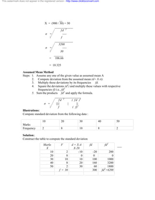
Method 2 :
Standard Deviation can be found out by using variables directly
Values (X)
X2
15 225
12 144
17 289
10 100
21 441
18 324
11 121
16 256
X = 120 X 2 = 1900
____________
X 2 - - X ¬ 2
ó = ---- ¦ --¦
N L N -
____________
1900 -120 ¬ 2
ó = ||| | - ||-
8 L 8 -
____________
ó = 237.5 - 225 = 3.53
(b) Deviation taken from assumed mean
This method is used when arithmetic mean is fractional value. A deviation from
fractional value leads to tedious task. To save calculation time, we apply this method.
The formula is
_________________
d 2 [ d ] 2
ó = --- - ¦ -- ¦
N [ N ]
Where d = Deviations from assumed mean = (X –A)
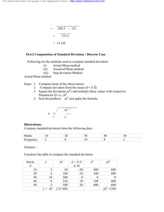
N = Number of observations](https://image.slidesharecdn.com/bcanumer-141110101906-conversion-gate02/85/Bca-numer-128-320.jpg)
![This watermark does not appear in the registered version - http://www.clicktoconvert.com
The following are the steps:
1. Assume any value which is very close to the given observations just by
inspection (A).
2. Find out the deviations from the assumed Mean . i.e., (X-A) denoted by d
3. Find out the sum of the deviations i.e., d
4. find out Square of the deviations; i.e., d 2
5. Apply all the values to the above mentioned formula.
Illustrations :
Compute the standard deviation of the following data:
Roll No. : 1 2 3 4 5 6 7 8 9 10
Marks : 45 50 56 63 68 78 74 66 72 33
Solution : (Construct the table to find out SD)
Roll No Marks (X) d = -A
d = X-50
d 2
1 45 45-50= -5 25
2 50 50-50= 0 0
3 56 6 36
4 63 13 169
5 68 18 324
6 78 28 784
7 74 24 576
8 66 16 256
9 72 22 484
10 33 -17 289
N=10
Total 110 2943
_________________
d 2 [ d ] 2
ó = --- - ¦ -- ¦
N [ N ]
_________________
2943 [ 110 ] 2
ó = --- - ¦ -- ¦
10 [ 10 ]
______________
= 294.3 - ( 11)2](https://image.slidesharecdn.com/bcanumer-141110101906-conversion-gate02/85/Bca-numer-129-320.jpg)