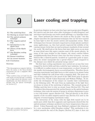
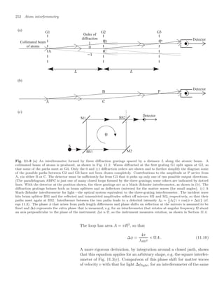
This document provides an overview of the Oxford Master Series in Physics textbook on Atomic Physics by C.J. Foot. It discusses the intended audience, topics covered, and structure of the textbook. Some key points: - The book is intended for final year undergraduate and beginning graduate students in physics. - It covers the core principles of atomic structure and selection of more advanced topics like laser spectroscopy, laser cooling, Bose-Einstein condensation, and quantum information processing with atoms. - The first six chapters cover basic atomic structure of hydrogen and helium using quantum mechanics. Later chapters discuss interactions with radiation and advanced experimental techniques. - Examples and problems are included throughout to illustrate concepts. Real experimental techniques

2. OXFORD MASTER SERIES IN PHYSICS

3. OXFORD MASTER SERIES IN PHYSICS
The Oxford Master Series is designed for final year undergraduate and beginning graduate students in
physics and related disciplines. It has been driven by a perceived gap in the literature today. While basic
undergraduate physics texts often show little or no connection with the huge explosion of research over the
last two decades, more advanced and specialized texts tend to be rather daunting for students. In this
series, all topics and their consequences are treated at a simple level, while pointers to recent developments
are provided at various stages. The emphasis in on clear physical principles like symmetry, quantum
mechanics, and electromagnetism which underlie the whole of physics. At the same time, the subjects are
related to real measurements and to the experimental techniques and devices currently used by physicists
in academe and industry. Books in this series are written as course books, and include ample tutorial
material, examples, illustrations, revision points, and problem sets. They can likewise be used as
preparation for students starting a doctorate in physics and related fields, or for recent graduates starting
research in one of these fields in industry.
CONDENSED MATTER PHYSICS
1. M. T. Dove: Structure and dynamics: an atomic view of materials
2. J. Singleton: Band theory and electronic properties of solids
3. A. M. Fox: Optical properties of solids
4. S. J. Blundell: Magnetism in condensed matter
5. J. F. Annett: Superconductivity
6. R. A. L. Jones: Soft condensed matter
ATOMIC, OPTICAL, AND LASER PHYSICS
7. C. J. Foot: Atomic physics
8. G. A. Brooker: Modern classical optics
9. S. M. Hooker, C. E. Webb: Laser physics
PARTICLE PHYSICS, ASTROPHYSICS, AND COSMOLOGY
10. D. H. Perkins: Particle astrophysics
11. Ta-Pei Cheng: Relativity, gravitation, and cosmology
STATISTICAL, COMPUTATIONAL, AND THEORETICAL PHYSICS
12. M. Maggiore: A modern introduction to quantum field theory
13. W. Krauth: Statistical mechanics: algorithms and computations
14. J. P. Sethna: Entropy, order parameters, and complexity

4. Atomic Physics
C. J. FOOT
Department of Physics
University of Oxford
1

5. 3
Great Clarendon Street, Oxford OX2 6DP
Oxford University Press is a department of the University of Oxford.
It furthers the University’s objective of excellence in research, scholarship,
and education by publishing worldwide in
Oxford New York
Auckland Cape Town Dar es Salaam Hong Kong Karachi
Kuala Lumpur Madrid Melbourne Mexico City Nairobi
New Delhi Shanghai Taipei Toronto
With offices in
Argentina Austria Brazil Chile Czech Republic France Greece
Guatemala Hungary Italy Japan South Korea Poland Portugal
Singapore Switzerland Thailand Turkey Ukraine Vietnam
Oxford is a registered trade mark of Oxford University Press
in the UK and in certain other countries
Published in the United States
by Oxford University Press Inc., New York
c
Oxford University Press 2005
The moral rights of the author have been asserted
Database right Oxford University Press (maker)
First published 2005
Reprinted 2005
All rights reserved. No part of this publication may be reproduced,
stored in a retrieval system, or transmitted, in any form or by any means,
without the prior permission in writing of Oxford University Press,
or as expressly permitted by law, or under terms agreed with the appropriate
reprographics rights organization. Enquiries concerning reproduction
outside the scope of the above should be sent to the Rights Department,
Oxford University Press, at the address above
You must not circulate this book in any other binding or cover
and you must impose this same condition on any acquirer
A catalogue record for this title
is available from the British Library
Library of Congress Cataloging in Publication Data
(Data available)
ISBN-10: 0 19 850695 3 (Hbk) Ean code 978 0 19 850695 9
ISBN-10: 0 19 850696 1 (Pbk) Ean code 978 0 19 850696 6
10 9 8 7 6 5 4 3 2
Typeset by Julie M. Harris using L
ATEX
Printed in Great Britain
on acid-free paper by Antony Rowe, Chippenham

6. Preface
This book is primarily intended to accompany an undergraduate course
in atomic physics. It covers the core material and a selection of more
advanced topics that illustrate current research in this field. The first
six chapters describe the basic principles of atomic structure, starting
in Chapter 1 with a review of the classical ideas. Inevitably the dis-
cussion of the structure of hydrogen and helium in these early chapters
has considerable overlap with introductory quantum mechanics courses,
but an understanding of these simple systems provides the basis for the
treatment of more complex atoms in later chapters. Chapter 7 on the
interaction of radiation with atoms marks the transition between the
earlier chapters on structure and the second half of the book which cov-
ers laser spectroscopy, laser cooling, Bose–Einstein condensation of di-
lute atomic vapours, matter-wave interferometry and ion trapping. The
exciting new developments in laser cooling and trapping of atoms and
Bose–Einstein condensation led to Nobel prizes in 1997 and 2001, respec-
tively. Some of the other selected topics show the incredible precision
that has been achieved by measurements in atomic physics experiments.
This theme is taken up in the final chapter that looks at quantum infor-
mation processing from an atomic physics perspective; the techniques
developed for precision measurements on atoms and ions give exquisite
control over these quantum systems and enable elegant new ideas from
quantum computation to be implemented.
The book assumes a knowledge of quantum mechanics equivalent to an
introductory university course, e.g. the solution of the Schrödinger equa-
tion in three dimensions and perturbation theory. This initial knowledge
will be reinforced by many examples in this book; topics generally re-
garded as difficult at the undergraduate level are explained in some de-
tail, e.g. degenerate perturbation theory. The hierarchical structure of
atoms is well described by perturbation theory since the different layers
of structure within atoms have considerably different energies associated
with them, and this is reflected in the names of the gross, fine and hyper-
fine structures. In the early chapters of this book, atomic physics may
appear to be simply applied quantum mechanics, i.e. we write down the
Hamiltonian for a given interaction and solve the Schrödinger equation
with suitable approximations. I hope that the study of the more ad-
vanced material in the later chapters will lead to a more mature and
deeper understanding of atomic physics. Throughout this book the ex-
perimental basis of atomic physics is emphasised and it is hoped that
the reader will gain some factual knowledge of atomic spectra.

7. vi Preface
The selection of topics from the diversity of current atomic physics
is necessarily subjective. I have concentrated on low-energy and high-
precision experiments which, to some extent, reflects local research in-
terests that are used as examples in undergraduate lectures at Oxford.
One of the selection criteria was that the material is not readily avail-
able in other textbooks, at the time of writing, e.g. atomic collisions
have not been treated in detail (only a brief summary of the scattering
of ultracold atoms is included in Chapter 10). Other notable omissions
include: X-ray spectra, which are discussed only briefly in connection
with the historically important work of Moseley, although they form an
important frontier of current research; atoms in strong laser fields and
plasmas; Rydberg atoms and atoms in doubly- and multiply-excited
states (e.g. excited by new synchrotron and free-electron laser sources);
and the structure and spectra of molecules.
I would like to thank Geoffrey Brooker for invaluable advice on physics
(in particular Appendix B) and on technical details of writing a textbook
for the Oxford Master Series. Keith Burnett, Jonathan Jones and An-
drew Steane have helped to clarify certain points, in my mind at least,
and hopefully also in the text. The series of lectures on laser cooling
given by William Phillips while he was a visiting professor in Oxford was
extremely helpful in the writing of the chapter on that topic. The fol-
lowing people provided very useful comments on the draft manuscript:
Rachel Godun, David Lucas, Mark Lee, Matthew McDonnell, Martin
Shotter, Claes-Göran Wahlström (Lund University) and the (anony-
mous) reviewers. Without the encouragement of Sönke Adlung at OUP
this project would not have been completed. Irmgard Smith drew some
of the diagrams. I am very grateful for the diagrams and data supplied
by colleagues, and reproduced with their permission, as acknowledged
in the figure captions. Several of the exercises on atomic structure de-
rive from Oxford University examination papers and it is not possible to
identify the examiners individually—some of these exam questions may
themselves have been adapted from some older sources of which I am
not aware.
Finally, I would like to thank Professors Derek Stacey, Joshua Silver
and Patrick Sandars who taught me atomic physics as an undergraduate
and graduate student in Oxford. I also owe a considerable debt to the
book on elementary atomic structure by Gordon Kemble Woodgate, who
was my predecessor as physics tutor at St Peter’s College, Oxford. In
writing this new text, I have tried to achieve the same high standards
of clarity and conciseness of expression whilst introducing new examples
and techniques from the laser era.
Background reading
It is not surprising that our language should be incapable of
describing the processes occurring with the atoms, for it was
invented to describe the experiences of daily life, and these
consist only of processes involving exceeding large numbers

8. vii
of atoms. Furthermore, it is very difficult to modify our
language so that it will be able to describe these atomic pro-
cesses, for words can only describe things of which we can
form mental pictures, and this ability, too, in the result of
daily experience. Fortunately, mathematics is not subject to
this limitation, and it has been possible to invent a mathe-
matical scheme—the quantum theory—which seems entirely
adequate for the treatment of atomic processes.
From The physical principles of the quantum theory, Werner
Heisenberg (1930).
The point of the excerpt is that quantum mechanics is essential for a
proper description of atomic physics and there are many quantum me-
chanics textbooks that would serve as useful background reading for this
book. The following short list includes those that the author found par-
ticularly relevant: Mandl (1992), Rae (1992) and Griffiths (1995). The
book Atomic spectra by Softley (1994) provides a concise introduction to
this field. The books Cohen-Tannoudji et al. (1977), Atkins (1983) and
Basdevant and Dalibard (2000) are very useful for reference and contain
many detailed examples of atomic physics. Angular-momentum theory
is very important for dealing with complicated atomic structures, but
it is beyond the intended level of this book. The classic book by Dirac
(1981) still provides a very readable account of the addition of angular
momenta in quantum mechanics. A more advanced treatment of atomic
structure can be found in Condon and Odabasi (1980), Cowan (1981)
and Sobelman (1996).
Oxford C. J. F.
Web site:
http://www.physics.ox.ac.uk/users/foot
This site has answers to some of the exercises, corrections and other
supplementary information.

9. This page intentionally left blank

10. Contents
1 Early atomic physics 1
1.1 Introduction 1
1.2 Spectrum of atomic hydrogen 1
1.3 Bohr’s theory 3
1.4 Relativistic effects 5
1.5 Moseley and the atomic number 7
1.6 Radiative decay 11
1.7 Einstein A and B coefficients 11
1.8 The Zeeman effect 13
1.8.1 Experimental observation of the Zeeman effect 17
1.9 Summary of atomic units 18
Exercises 19
2 The hydrogen atom 22
2.1 The Schrödinger equation 22
2.1.1 Solution of the angular equation 23
2.1.2 Solution of the radial equation 26
2.2 Transitions 29
2.2.1 Selection rules 30
2.2.2 Integration with respect to θ 32
2.2.3 Parity 32
2.3 Fine structure 34
2.3.1 Spin of the electron 35
2.3.2 The spin–orbit interaction 36
2.3.3 The fine structure of hydrogen 38
2.3.4 The Lamb shift 40
2.3.5 Transitions between fine-structure levels 41
Further reading 42
Exercises 42
3 Helium 45
3.1 The ground state of helium 45
3.2 Excited states of helium 46
3.2.1 Spin eigenstates 51
3.2.2 Transitions in helium 52
3.3 Evaluation of the integrals in helium 53
3.3.1 Ground state 53
3.3.2 Excited states: the direct integral 54
3.3.3 Excited states: the exchange integral 55

11. x Contents
Further reading 56
Exercises 58
4 The alkalis 60
4.1 Shell structure and the periodic table 60
4.2 The quantum defect 61
4.3 The central-field approximation 64
4.4 Numerical solution of the Schrödinger equation 68
4.4.1 Self-consistent solutions 70
4.5 The spin–orbit interaction: a quantum mechanical
approach 71
4.6 Fine structure in the alkalis 73
4.6.1 Relative intensities of fine-structure transitions 74
Further reading 75
Exercises 76
5 The LS-coupling scheme 80
5.1 Fine structure in the LS-coupling scheme 83
5.2 The jj-coupling scheme 84
5.3 Intermediate coupling: the transition between coupling
schemes 86
5.4 Selection rules in the LS-coupling scheme 90
5.5 The Zeeman effect 90
5.6 Summary 93
Further reading 94
Exercises 94
6 Hyperfine structure and isotope shift 97
6.1 Hyperfine structure 97
6.1.1 Hyperfine structure for s-electrons 97
6.1.2 Hydrogen maser 100
6.1.3 Hyperfine structure for l = 0 101
6.1.4 Comparison of hyperfine and fine structures 102
6.2 Isotope shift 105
6.2.1 Mass effects 105
6.2.2 Volume shift 106
6.2.3 Nuclear information from atoms 108
6.3 Zeeman effect and hyperfine structure 108
6.3.1 Zeeman effect of a weak field, µBB A 109
6.3.2 Zeeman effect of a strong field, µBB A 110
6.3.3 Intermediate field strength 111
6.4 Measurement of hyperfine structure 112
6.4.1 The atomic-beam technique 114
6.4.2 Atomic clocks 118
Further reading 119
Exercises 120
7 The interaction of atoms with radiation 123
7.1 Setting up the equations 123

12. Contents xi
7.1.1 Perturbation by an oscillating electric field 124
7.1.2 The rotating-wave approximation 125
7.2 The Einstein B coefficients 126
7.3 Interaction with monochromatic radiation 127
7.3.1 The concepts of π-pulses and π/2-pulses 128
7.3.2 The Bloch vector and Bloch sphere 128
7.4 Ramsey fringes 132
7.5 Radiative damping 134
7.5.1 The damping of a classical dipole 135
7.5.2 The optical Bloch equations 137
7.6 The optical absorption cross-section 138
7.6.1 Cross-section for pure radiative broadening 141
7.6.2 The saturation intensity 142
7.6.3 Power broadening 143
7.7 The a.c. Stark effect or light shift 144
7.8 Comment on semiclassical theory 145
7.9 Conclusions 146
Further reading 147
Exercises 148
8 Doppler-free laser spectroscopy 151
8.1 Doppler broadening of spectral lines 151
8.2 The crossed-beam method 153
8.3 Saturated absorption spectroscopy 155
8.3.1 Principle of saturated absorption spectroscopy 156
8.3.2 Cross-over resonances in saturation spectroscopy 159
8.4 Two-photon spectroscopy 163
8.5 Calibration in laser spectroscopy 168
8.5.1 Calibration of the relative frequency 168
8.5.2 Absolute calibration 169
8.5.3 Optical frequency combs 171
Further reading 175
Exercises 175
9 Laser cooling and trapping 178
9.1 The scattering force 179
9.2 Slowing an atomic beam 182
9.2.1 Chirp cooling 184
9.3 The optical molasses technique 185
9.3.1 The Doppler cooling limit 188
9.4 The magneto-optical trap 190
9.5 Introduction to the dipole force 194
9.6 Theory of the dipole force 197
9.6.1 Optical lattice 201
9.7 The Sisyphus cooling technique 203
9.7.1 General remarks 203
9.7.2 Detailed description of Sisyphus cooling 204
9.7.3 Limit of the Sisyphus cooling mechanism 207

13. xii Contents
9.8 Raman transitions 208
9.8.1 Velocity selection by Raman transitions 208
9.8.2 Raman cooling 210
9.9 An atomic fountain 211
9.10 Conclusions 213
Exercises 214
10 Magnetic trapping, evaporative cooling and
Bose–Einstein condensation 218
10.1 Principle of magnetic trapping 218
10.2 Magnetic trapping 220
10.2.1 Confinement in the radial direction 220
10.2.2 Confinement in the axial direction 221
10.3 Evaporative cooling 224
10.4 Bose–Einstein condensation 226
10.5 Bose–Einstein condensation in trapped atomic vapours 228
10.5.1 The scattering length 229
10.6 A Bose–Einstein condensate 234
10.7 Properties of Bose-condensed gases 239
10.7.1 Speed of sound 239
10.7.2 Healing length 240
10.7.3 The coherence of a Bose–Einstein condensate 240
10.7.4 The atom laser 242
10.8 Conclusions 242
Exercises 243
11 Atom interferometry 246
11.1 Young’s double-slit experiment 247
11.2 A diffraction grating for atoms 249
11.3 The three-grating interferometer 251
11.4 Measurement of rotation 251
11.5 The diffraction of atoms by light 253
11.5.1 Interferometry with Raman transitions 255
11.6 Conclusions 257
Further reading 258
Exercises 258
12 Ion traps 259
12.1 The force on ions in an electric field 259
12.2 Earnshaw’s theorem 260
12.3 The Paul trap 261
12.3.1 Equilibrium of a ball on a rotating saddle 262
12.3.2 The effective potential in an a.c. field 262
12.3.3 The linear Paul trap 262
12.4 Buffer gas cooling 266
12.5 Laser cooling of trapped ions 267
12.6 Quantum jumps 269
12.7 The Penning trap and the Paul trap 271

14. Contents xiii
12.7.1 The Penning trap 272
12.7.2 Mass spectroscopy of ions 274
12.7.3 The anomalous magnetic moment of the electron 274
12.8 Electron beam ion trap 275
12.9 Resolved sideband cooling 277
12.10 Summary of ion traps 279
Further reading 279
Exercises 280
13 Quantum computing 282
13.1 Qubits and their properties 283
13.1.1 Entanglement 284
13.2 A quantum logic gate 287
13.2.1 Making a CNOT gate 287
13.3 Parallelism in quantum computing 289
13.4 Summary of quantum computers 291
13.5 Decoherence and quantum error correction 291
13.6 Conclusion 293
Further reading 294
Exercises 294
A Appendix A: Perturbation theory 298
A.1 Mathematics of perturbation theory 298
A.2 Interaction of classical oscillators of similar frequencies 299
B Appendix B: The calculation of electrostatic energies 302
C Appendix C: Magnetic dipole transitions 305
D Appendix D: The line shape in saturated absorption
spectroscopy 307
E Appendix E: Raman and two-photon transitions 310
E.1 Raman transitions 310
E.2 Two-photon transitions 313
F Appendix F: The statistical mechanics of
Bose–Einstein condensation 315
F.1 The statistical mechanics of photons 315
F.2 Bose–Einstein condensation 316
F.2.1 Bose–Einstein condensation in a harmonic trap 318
References 319
Index 326

15. This page intentionally left blank

16. Early atomic physics
1
1.1 Introduction 1
1.2 Spectrum of atomic
hydrogen 1
1.3 Bohr’s theory 3
1.4 Relativistic effects 5
1.5 Moseley and the atomic
number 7
1.6 Radiative decay 11
1.7 Einstein A and B
coefficients 11
1.8 The Zeeman effect 13
1.9 Summary of atomic units 18
Exercises 19
1.1 Introduction
The origins of atomic physics were entwined with the development of
quantum mechanics itself ever since the first model of the hydrogen
atom by Bohr. This introductory chapter surveys some of the early
ideas, including Einstein’s treatment of the interaction of atoms with
radiation, and a classical treatment of the Zeeman effect. These meth-
ods, developed before the advent of the Schrödinger equation, remain
useful as an intuitive way of thinking about atomic structure and tran-
sitions between the energy levels. The ‘proper’ description in terms of
atomic wavefunctions is presented in subsequent chapters.
Before describing the theory of an atom with one electron, some ex-
perimental facts are presented. This ordering of experiment followed
by explanation reflects the author’s opinion that atomic physics should
not be presented as applied quantum mechanics, but it should be mo-
tivated by the desire to understand experiments. This represents what
really happens in research where most advances come about through the
interplay of theory and experiment.
1.2 Spectrum of atomic hydrogen
It has long been known that the spectrum of light emitted by an element
is characteristic of that element, e.g. sodium in a street lamp, or burn-
ing in a flame, produces a distinctive yellow light. This crude form of
spectroscopy, in which the colour is seen by eye, formed the basis for a
simple chemical analysis. A more sophisticated approach using a prism,
or diffraction grating, to disperse the light inside a spectrograph shows
that the characteristic spectrum for atoms is composed of discrete lines
that are the ‘fingerprint’ of the element. As early as the 1880s, Fraun-
hofer used a spectrograph to measure the wavelength of lines, that had
not been seen before, in light from the sun and he deduced the exis-
tence of a new element called helium. In contrast to atoms, the spectra
of molecules (even the simplest diatomic ones) contain many closely-
spaced lines that form characteristic molecular bands; large molecules,
and solids, usually have nearly continuous spectra with few sharp fea-
tures. In 1888, the Swedish professor J. Rydberg found that the spectral

17. 2 Early atomic physics
lines in hydrogen obey the following mathematical formula:
1
λ
= R
1
n2
−
1
n2
, (1.1)
where n and n
are whole numbers; R is a constant that has become
known as the Rydberg constant. The series of spectral lines for which
n = 2 and n
= 3, 4, . . . is now called the Balmer series and lies in the
visible region of the spectrum.1
The first line at 656 nm is called the
1
The Swiss mathematician Johann
Balmer wrote down an expression
which was a particular case of eqn 1.1
with n = 2, a few years before Jo-
hannes (commonly called Janne) Ry-
dberg found the general formula that
predicted other series.
Balmer-α (or Hα) line and it gives rise to the distinctive red colour of
a hydrogen discharge—a healthy red glow indicates that most of the
molecules of H2 have been dissociated into atoms by being bombarded
by electrons in the discharge. The next line in the series is the Balmer-β
line at 486 nm in the blue and subsequent lines at shorter wavelengths
tend to a limit in the violet region.2
To describe such series of lines it is
2
A spectrum of the Balmer series of
lines is on the cover of this book. convenient to define the reciprocal of the transition wavelength as the
wavenumber ν̃ that has units of m−1
(or often cm−1
),
ν̃ =
1
λ
. (1.2)
Wavenumbers may seem rather old-fashioned but they are very useful
in atomic physics since they are easily evaluated from measured wave-
lengths without any conversion factor. In practice, the units used for
a given quantity are related to the method used to measure it, e.g.
spectroscopes and spectrographs are calibrated in terms of wavelength.3
3
In this book transitions are also spec-
ified in terms of their frequency (de-
noted by f so that f = cν̃), or in elec-
tron volts (eV) where appropriate.
A photon with wavenumber ν̃ has energy E = hcν̃. The Balmer for-
mula implicitly contains a more general empirical law called the Ritz
combination principle that states: the wavenumbers of certain lines in
the spectrum can be expressed as sums (or differences) of other lines:
ν̃3 = ν̃1 ±ν̃2, e.g. the wavenumber of the Balmer-β line (n = 2 to n
= 4)
is the sum of that for Balmer-α (n = 2 to n
= 3) and the first line in
the Paschen series (n = 3 to n
= 4). Nowadays this seems obvious
since we know about the underlying energy-level structure of atoms but
it is still a useful principle for analyzing spectra. Examination of the
sums and differences of the wavenumbers of transitions gives clues that
enable the underlying structure to be deduced, rather like a crossword
puzzle—some examples of this are given in later chapters. The observed
spectral lines in hydrogen can all be expressed as differences between
energy levels, as shown in Fig. 1.1, where the energies are proportional
to 1/n2
. Other series predicted by eqn 1.1 were more difficult to observe
experimentally than the Balmer series. The transitions to n = 1 give
the Lyman series in the vacuum ultraviolet region of the spectrum.4
The
4
Air absorbs radiation at wavelengths
shorter than about 200 nm and so
spectrographs must be evacuated, as
well as being made with special optics.
series of lines with wavelengths longer than the Balmer series lie in the
infra-red region (not visible to the human eye, nor readily detected by
photographic film—the main methods available to the early spectroscop-
ists). The following section looks at how these spectra can be explained
theoretically.

18. 1.3 Bohr’s theory 3
Fig. 1.1 The energy levels of the hydro-
gen atom. The transitions from higher
shells n = 2, 3, 4, . . . down to the n = 1
shell give the Lyman series of spectral
lines. The series of lines formed by
transitions to other shells are: Balmer
(n = 2), Paschen (n = 3), Brack-
ett (n = 4) and Pfund (n = 5) (the
last two are not labelled in the figure).
Within each series the lines are denoted
by Greek letters, e.g. Lα for n = 2 to
n = 1 and Hβ for n = 4 to n = 2.
1.3 Bohr’s theory
In 1913, Bohr put forward a radical new model of the hydrogen atom
using quantum mechanics. It was known from Rutherford’s experiments
that inside atoms there is a very small, dense nucleus with a positive
charge. In the case of hydrogen this is a single proton with a single elec-
tron bound to it by the Coulomb force. Since the force is proportional
to 1/r2
, as for gravity, the atom can be considered in classical terms as
resembling a miniature solar system with the electron orbiting around
the proton, just like a planet going around the sun. However, quantum
mechanics is important in small systems and only certain electron orbits
are allowed. This can be deduced from the observation that hydrogen
atoms emit light only at particular wavelengths corresponding to tran-
sitions between discrete energies. Bohr was able to explain the observed
spectrum by introducing the then novel idea of quantisation that goes
beyond any previous classical theory. He took the orbits that occur in
classical mechanics and imposed quantisation rules onto them.
Bohr assumed that each electron orbits the nucleus in a circle, whose
radius r is determined by the balance between centripetal acceleration
and the Coulomb attraction towards the proton. For electrons of mass
me and speed v this gives
mev2
r
=
e2
4π0r2
. (1.3)
In SI units the strength of the electrostatic interaction between two

19. 4 Early atomic physics
charges of magnitude e is characterised by the combination of constants
e2
/4π0.5
This leads to the following relation between the angular fre-
5
Older systems of units give more suc-
cinct equations without 4π0; some of
this neatness can be retained by keep-
ing e2/4π0 grouped together.
quency ω = v/r and the radius:
ω2
=
e2
/4π0
mer3
. (1.4)
This is equivalent to Kepler’s laws for planetary orbits relating the square
of the period 2π/ω to the cube of the radius (as expected since all steps
have been purely classical mechanics). The total energy of an electron
in such an orbit is the sum of its kinetic and potential energies:
E =
1
2
mev2
−
e2
/4π0
r
. (1.5)
Using eqn 1.3 we find that the kinetic energy has a magnitude equal
to half the potential energy (an example of the virial theorem). Taking
into account the opposite signs of kinetic and potential energy, we find
E = −
e2
/4π0
2r
. (1.6)
This total energy is negative because the electron is bound to the proton
and energy must be supplied to remove it. To go further Bohr made the
following assumption.
Assumption I There are certain allowed orbits for which the electron
has a fixed energy. The electron loses energy only when it jumps between
the allowed orbits and the atom emits this energy as light of a given
wavelength.
That electrons in the allowed orbits do not radiate energy is contrary
to classical electrodynamics—a charged particle in circular motion un-
dergoes acceleration and hence radiates electromagnetic waves. Bohr’s
model does not explain why the electron does not radiate but simply
takes this as an assumption that turns out to agree with the experi-
mental data. We now need to determine which out of all the possible
classical orbits are the allowed ones. There are various ways of doing this
and we follow the standard method, used in many elementary texts, that
assumes quantisation of the angular momentum in integral multiples of
(Planck’s constant over 2π):
mevr = n , (1.7)
where n is an integer. Combining this with eqn 1.3 gives the radii of the
allowed orbits as
r = a0n2
, (1.8)
where the Bohr radius a0 is given by
a0 =
2
(e2/4π0) me
. (1.9)
This is the natural unit of length in atomic physics. Equations 1.6 and
1.8 combine to give the famous Bohr formula:
E = −
e2
/4π0
2a0
1
n2
. (1.10)

20. 1.4 Relativistic effects 5
The positive integer n is called the principal quantum number.6 6
The alert reader may wonder why
this is true since we introduced n in
connection with angular momentum in
eqn 1.7, and (as shown later) elec-
trons can have zero angular momen-
tum. This arises from the simplifica-
tion of Bohr’s theory. Exercise 1.12 dis-
cusses a more satisfactory, but longer
and subtler, derivation that is closer to
Bohr’s original papers. However, the
important thing to remember from this
introduction is not the formalism but
the magnitude of the atomic energies
and sizes.
Bohr’s formula predicts that in the transitions between these energy
levels the atoms emit light with a wavenumber given by
ν̃ = R∞
1
n2
−
1
n2
. (1.11)
This equation fits very closely to the observed spectrum of atomic hy-
drogen described by eqn 1.1. The Rydberg constant R∞ in eqn 1.11 is
defined by
hcR∞ =
e2
/4π0
2
me
22
. (1.12)
The factor of hc multiplying the Rydberg constant is the conversion fac-
tor between energy and wavenumbers since the value of R∞ is given
in units of m−1
(or cm−1
in commonly-used units). The measure-
ment of the spectrum of atomic hydrogen using laser techniques has
given an extremely accurate value for the Rydberg constant7
R∞ = 7
This is the 2002 CODATA recom-
mended value. The currently accepted
values of physical constants can be
found on the web site of the National
Institute of Science and Technology
(NIST).
10 973 731.568 525 m−1
. However, there is a subtle difference between
the Rydberg constant calculated for an electron orbiting a fixed nucleus
R∞ and the constant for real hydrogen atoms in eqn 1.1 (we originally
wrote R without a subscript but more strictly we should specify that
it is the constant for hydrogen RH). The theoretical treatment above
has assumed an infinitely massive nucleus, hence the subscript ∞. In
reality both the electron and proton move around the centre of mass of
the system. For a nucleus of finite mass M the equations are modified
by replacing the electron mass me by its reduced mass
m =
meM
me + M
. (1.13)
For hydrogen
RH = R∞
Mp
me + Mp
R∞
1 −
me
Mp
, (1.14)
where the electron-to-proton mass ratio is me/Mp 1/1836. This
reduced-mass correction is not the same for different isotopes of an el-
ement, e.g. hydrogen and deuterium. This leads to a small but readily
observable difference in the frequency of the light emitted by the atoms
of different isotopes; this is called the isotope shift (see Exercises 1.1 and
1.2).
1.4 Relativistic effects
Bohr’s theory was a great breakthrough. It was such a radical change
that the fundamental idea about the quantisation of the orbits was at
first difficult for people to appreciate—they worried about how the elec-
trons could know which orbits they were going into before they jumped.
It was soon realised, however, that the assumption of circular orbits is

21. 6 Early atomic physics
too much of an over-simplification. Sommerfeld produced a quantum
mechanical theory of electrons in elliptical orbits that was consistent
with special relativity. He introduced quantisation through a general
rule that stated ‘the integral of the momentum associated with a coor-
dinate around one period of the motion associated with that coordinate
is an integral multiple of Planck’s constant’. This general method can
be applied to any physical system where the classical motion is periodic.
Applying this quantisation rule to momentum around a circular orbit
gives the equivalent of eqn 1.7:8
8
This has a simple interpretation in
terms of the de Broglie wavelength
associated with an electron λdB =
h/mev. The allowed orbits are those
that have an integer multiple of de
Broglie wavelengths around the circum-
ference: 2πr = nλdB, i.e. they are
standing matter waves. Curiously, this
idea has some resonance with modern
ideas in string theory.
mev × 2πr = nh . (1.15)
In addition to quantising the motion in the coordinate θ, Sommerfeld
also considered quantisation of the radial degree of freedom r. He found
that some of the elliptical orbits expected for a potential proportional
to 1/r are also stationary states (some of the allowed orbits have a high
eccentricity, more like those of comets than planets). Much effort was
put into complicated schemes based on classical orbits with quantisation,
and by incorporating special relativity this ‘old quantum theory’ could
explain accurately the fine structure of spectral lines. The exact details
of this work are now mainly of historical interest but it is worthwhile
to make a simple estimate of relativistic effects. In special relativity a
particle of rest mass m moving at speed v has an energy
E (v) = γ mc2
, (1.16)
where the gamma factor is γ = 1/
1 − v2/c2. The kinetic energy of the
moving particle is ∆E = E (v) − E(0) = (γ − 1) mec2
. Thus relativistic
effects produce a fractional change in energy:9
9
We neglect a factor of 1
2
in the bino-
mial expansion of the expression for γ
at low speeds, v2/c2 1. ∆E
E
v2
c2
. (1.17)
This leads to energy differences between the various elliptical orbits of
the same gross energy because the speed varies in different ways around
the elliptical orbits, e.g. for a circular orbit and a highly elliptical orbit
of the same gross energy. From eqns 1.3 and 1.7 we find that the ratio
of the speed in the orbit to the speed of light is
v
c
=
α
n
, (1.18)
where the fine-structure constant α is given by
α =
e2
/4π0
c
. (1.19)
This fundamental constant plays an important role throughout atomic
physics.10
Numerically its value is approximately α 1/137 (see inside
10
An electron in the Bohr orbit with
n = 1 has speed αc. Hence it has linear
momentum meαc and angular momen-
tum meαca0 = .
the back cover for a list of constants used in atomic physics). From
eqn 1.17 we see that relativistic effects lead to energy differences of
order α2
times the gross energy. (This crude estimate neglects some

22. 1.5 Moseley and the atomic number 7
dependence on principal quantum number and Chapter 2 gives a more
quantitative treatment of this fine structure.) It is not necessary to go
into all the refinements of Sommerfeld’s relativistic theory that gave
the energy levels in hydrogen very precisely, by imposing quantisation
rules on classical orbits, since ultimately a paradigm shift was neces-
sary. Those ideas were superseded by the use of wavefunctions in the
Schrödinger equation. The idea of elliptical orbits provides a connection
with our intuition based on classical mechanics and we often retain some
traces of this simple picture of electron orbits in our minds. However,
for atoms with more than one electron, e.g. helium, classical models do
not work and we must think in terms of wavefunctions.
1.5 Moseley and the atomic number
At the same time as Bohr was working on his model of the hydrogen
atom, H. G. J. Moseley measured the X-ray spectra of many elements.
Moseley established that the square root of the frequency of the emitted
lines is proportional to the atomic number Z (that he defined as the
position of the atom in the periodic table, starting counting at Z = 1
for hydrogen), i.e.
f ∝ Z . (1.20)
Moseley’s original plot is shown in Fig. 1.2. As we shall see, this equation
is a considerable simplification of the actual situation but it was remark-
ably powerful at the time. By ordering the elements using Z rather than
relative atomic mass, as was done previously, several inconsistencies in
the periodic table were resolved. There were still gaps that were later
filled by the discovery of new elements. In particular, for the rare-earth
elements that have similar chemical properties and are therefore difficult
to distinguish, it was said ‘in an afternoon, Moseley could solve the prob-
lem that had baffled chemists for many decades and establish the true
number of possible rare earths’ (Segrè 1980). Moseley’s observations can
be explained by a relatively simple model for atoms that extends Bohr’s
model for hydrogen.11 11
Tragically, Henry Gwyn Jeffreys
Moseley was killed when he was only
28 while fighting in the First World War
(see the biography by Heilbron (1974)).
A natural way to extend Bohr’s atomic model to heavier atoms is
to suppose that the electrons fill up the allowed orbits starting from
the bottom. Each energy level only has room for a certain number of
electrons so they cannot all go into the lowest level and they arrange
themselves in shells, labelled by the principal quantum number, around
the nucleus. This shell structure arises because of the Pauli exclusion
principle and the electron spin, but for now let us simply consider it as an
empirical fact that the maximum number of electrons in the n = 1 shell
is 2, the n = 2 shell has 8 and the n = 3 shell has 18, etc. For historical
reasons, X-ray spectroscopists do not use the principal quantum number
but label the shells by letters: K for n = 1, L for n = 2, M for n = 3
and so on alphabetically.12
This concept of electronic shells explains the
12
The chemical properties of the ele-
ments depend on this electronic struc-
ture, e.g. the inert gases have full shells
of electrons and these stable configura-
tions are not willing to form chemical
bonds. The explanation of the atomic
structure underlying the periodic ta-
ble is discussed further in Section 4.1.
See also Atkins (1994) and Grant and
Phillips (2001).
emission of X-rays from atoms in the following way. Moseley produced
X-rays by bombarding samples of the given element with electrons that

23. 8 Early atomic physics
79.Au.
78.Pt.
77.Ir.
76.Os.
75.
74.W.
73.Ta.
72.
71.Lu.
70.Ny.
69.Tm.
68.Er.
67.Ho.
66.Ds.
65.Tb.
64.Gd.
63.Eu.
62.Sa.
61.
60.Nd.
59.Pr.
58.Ce.
57.La.
56.Ba.
55.Cs.
54.Xe.
53.I.
52.Te.
51.Sb.
50.Sn.
49.In.
48.Cd.
47.Ag.
46.Pd.
45.Rh.
44.Ru.
43.
42.Mo.
41.Nb.
40.Zr.
39.Y.
38.Sr.
37.Rb.
36.Kr.
35.Br.
34.Se.
33.As.
32.Ge.
31.Ga.
30.Zn
29.Cu.
28.Ni.
27.Co.
26.Fe.
25.Mn.
24.Cr.
23.V.
22.Ti.
21.Sc.
20.Ca.
19.K.
18.A.
17.Cl.
16.S.
15.P.
14.Si.
13.Al.
.
8 6 5 4 3 2 1.5 1 0.9 0.8 0.7 0.6
6 8 10 12 14 16 18 20 22 24
Fig. 1.2 Moseley’s plot of the square root of the frequency of X-ray lines of elements
against their atomic number. Moseley’s work established the atomic number Z as
a more fundamental quantity than the ‘atomic weight’ (now called relative atomic
mass). Following modern convention the units of the horizontal scales would be
(108
√
Hz) at the bottom and (10−10 m) for the log scale at the top. (Archives of the
Clarendon Laboratory, Oxford; also shown on the Oxford physics web site.)13
13
The handwriting in the bottom right
corner states that this diagram is the
original for Moseley’s famous paper in
Phil. Mag., 27, 703 (1914).

24. 1.5 Moseley and the atomic number 9
had been accelerated to a high voltage in a vacuum tube. These fast
electrons knock an electron out of an atom in the sample leaving a
vacancy or hole in one of its shells. This allows an electron from a
higher-lying shell to ‘fall down’ to fill this hole emitting radiation of a
wavelength corresponding to the difference in energy between the shells.
To explain Moseley’s observations quantitatively we need to modify
the equations in Section 1.3, on Bohr’s theory, to account for the effect
of a nucleus of charge greater than the +1e of the proton. For a nuclear
charge Ze we replace e2
/4π0 by Ze2
/4π0 in all the equations, resulting
in a formula for the energies like that of Balmer but multiplied by a factor
of Z2
. This dependence on the square of the atomic number means that,
for all but the lightest elements, transitions between low-lying shells lead
to emission of radiation in the X-ray region of the spectrum. Scaling the
Bohr theory result is accurate for hydrogenic ions, i.e. systems with
one electron around a nucleus of charge Ze. In neutral atoms the other
electrons (that do not jump) are not simply passive spectators but partly
screen the nuclear charge; for a given X-ray line, say the K- to L-shell
transition, a more accurate formula is
1
λ
= R∞
(Z − σK)2
12
−
(Z − σL)2
22
. (1.21)
The screening factors σK and σL are not entirely independent of Z and
the values of these screening factors for each shell vary slightly (see the
exercises at the end of this chapter). For large atomic numbers this
formula tends to eqn 1.20 (see Exercise 1.4). This simple approach does
not explain why the screening factor for a shell can exceed the number
of electrons inside that shell, e.g. σK = 2 for Z = 74 although only
one electron remains in this shell when a hole is formed. This does not
make sense in a classical model with electrons orbiting around a nucleus,
but can be explained by atomic wavefunctions—an electron with a high
principal quantum number (and little angular momentum) has a finite
probability of being found at small radial distances.
The study of X-rays has developed into a whole field of its own within
atomic physics, astrophysics and condensed matter, but there is only
room to mention a few brief facts here. When an electron is removed
from the K-shell the atom has an amount of energy equal to its bind-
ing energy, i.e. a positive amount of energy, and it is therefore usual
to draw the diagram with the K-shell at the top, as in Fig. 1.3. These
are the energy levels of the hole in the electron shells. This diagram
shows why the creation of a hole in a low-lying shell leads to a succes-
sion of transitions as the hole works its way outwards through the shells.
The hole (or equivalently the falling electron) can jump more than one
shell at a time; each line in a series from a given shell is labelled using
Greek letters (as in the series in hydrogen), e.g. Kα, Kβ, . . .. The levels
drawn in Fig. 1.3 have some sub-structure and this leads to transitions
with slightly different wavelengths, as shown in Moseley’s plot. This is
fine structure caused by relativistic effects that we considered for Som-
merfeld’s theory; the substitution e2
/4π0 → Ze2
/4π0, as above, (or

25. 10 Early atomic physics
Fig. 1.3 The energy levels of the inner
shells of the tungsten atom (Z = 74)
and the transitions between them that
give rise to X-rays. The level scheme
has several important differences from
that for the hydrogen atom (Fig. 1.1).
Firstly, the energies are tens of keV,
as compared to eV for Z = 1, be-
cause they scale as Z2 (approximately).
Secondly, the energy levels are plotted
with n = 1 at the top because when
an electron is removed from the K-shell
the system has more energy than the
neutral atom; energies are shown for
an atom with a vacancy (missing elec-
tron) in the K-, L-, M- and N-shells.
The atom emits X-ray radiation when
an electron drops down from a higher
shell to fill a vacancy in a lower shell—
this process is equivalent to the va-
cancy, or hole, working its way out-
wards. This way of plotting the ener-
gies of the system shows clearly that
the removal of an electron from the K-
shell leads to a cascade of X-ray tran-
sitions, e.g. a transition between the
n = 1 and 2 shells gives a line in the
K-series which is followed by a line in
another series (L-, M-, etc.). When the
vacancy reaches the outermost shells of
electrons that are only partially filled
with valence electrons with binding en-
ergies of a few eV (the O- and P-shells
in the case of tungsten), the transition
energies become negligible compared to
those between the inner shells. This
level scheme is typical for electrons in a
moderately heavy atom, i.e. one with
filled K-, L-, M- and N-shells. (The
lines of the L-series shown dotted are
allowed X-ray transitions, but they do
not occur following Kα emission.)
equivalently α → Zα) shows that fine structure is of order (Zα)2
times
the gross structure, which itself is proportional to Z2
. Thus relativistic
effects grow as Z4
and become very significant for the inner electrons of
heavy atoms, leading to the fine structure of the L- and M-shells seen in
Fig. 1.3. This relativistic splitting of the shells explains why in Mose-
ley’s plot (Fig. 1.2) there are two closely-spaced curves for the Kα-line,
and several curves for the L-series.
Nowadays much of the X-ray work in atomic physics is carried out
using sources such as synchrotrons; these devices accelerate electrons by
the techniques used in particle accelerators. A beam of high-energy elec-
trons circulates in a ring and the circular motion causes the electrons to

26. 1.7 Einstein A and B coefficients 11
radiate X-rays. Such a source can be used to obtain an X-ray absorption
spectrum.14
There are many other applications of X-ray emission, e.g. 14
Absorption is easier to interpret than
emission since only one of the terms
in eqn 1.21 is important, e.g. EK =
hcR∞(Z − σK)2.
as a diagnostic tool for the processes that occur in plasmas in fusion
research and in astrophysical objects. Many interesting processes occur
at ‘high energies’ in atomic physics but the emphasis in this book is
mainly on lower energies.
1.6 Radiative decay
An electric dipole moment −ex0 oscillating at angular frequency ω ra-
diates a power15
15
This total power equals the integral
of the Poynting vector over a closed sur-
face in the far-field of radiation from the
dipole. This is calculated from the os-
cillating electric and magnetic fields in
this region (see electromagnetism texts
or Corney (2000)).
P =
e2
x2
0ω4
12π0c3
. (1.22)
An electron in harmonic motion has a total energy16
of E = meω2
x2
0/2,
16
The sum of the kinetic and potential
energies.
where x0 is the amplitude of the motion. This energy decreases at a rate
equal to the power radiated:
dE
dt
= −
e2
ω2
6π0mec3
E = −
E
τ
, (1.23)
where the classical radiative lifetime τ is given by
1
τ
=
e2
ω2
6π0mec3
. (1.24)
For the transition in sodium at a wavelength of 589 nm (yellow light)
this equation predicts a value of τ = 16 ns 10−8
s. This is very close
to the experimentally measured value and typical of allowed transitions
that emit visible light. Atomic lifetimes, however, vary over a very wide
range,17
e.g. for the Lyman-α transition (shown in Fig. 1.1) the upper
17
The classical lifetime scales as 1/ω2.
However, we will find that the quantum
mechanical result is different (see Exer-
cise 1.8).
level has a lifetime of only a few nanoseconds.18,19
18
Higher-lying levels, e.g. n = 30,
live for many microseconds (Gallagher
1994).
19
Atoms can be excited up to config-
urations with high principal quantum
numbers in laser experiments; such sys-
tems are called Rydberg atoms and
have small intervals between their en-
ergy levels. As expected from the cor-
respondence principle, these Rydberg
atoms can be used in experiments that
probe the interface between classical
and quantum mechanics.
The classical value of the lifetime gives the fastest time in which the
atom could decay on a given transition and this is often close to the
observed lifetime for strong transitions. Atoms do not decay faster than
a classical dipole radiating at the same wavelength, but they may decay
more slowly (by many orders of magnitude in the case of forbidden
transitions).20
20
The ion-trapping techniques de-
scribed in Chapter 12 can probe tran-
sitions with spontaneous decay rates
less than 1 s−1, using single ions con-
fined by electric and magnetic fields—
something that was only a ‘thought
experiment’ for Bohr and the other
founders of quantum theory. In par-
ticular, the effect of individual quan-
tum jumps between atomic energy lev-
els is observed. Radiative decay resem-
bles radioactive decay in that individ-
ual atoms spontaneously emit a photon
at a given time but taking the average
over an ensemble of atoms gives expo-
nential decay.
1.7 Einstein A and B coefficients
The development of the ideas of atomic structure was linked to exper-
iments on the emission, and absorption, of radiation from atoms, e.g.
X-rays or light. The emission of radiation was considered as something
that just has to happen in order to carry away the energy when an elec-
tron jumps from one allowed orbit to another, but the mechanism was
not explained.21
In one of his many strokes of genius Einstein devised a
21
A complete explanation of sponta-
neous emission requires quantum elec-
trodynamics.
way of treating the phenomenon of spontaneous emission quantitatively,

27. 12 Early atomic physics
based on an intuitive understanding of the process.22
22
This treatment of the interaction of
atoms with radiation forms the founda-
tion for the theory of the laser, and is
used whenever radiation interacts with
matter (see Fox 2001). A historical ac-
count of Einstein’s work and its pro-
found implications can be found in Pais
(1982).
Einstein considered atoms with two levels of energies, E1 and E2, as
shown in Fig. 1.4; each level may have more than one state and the
number of states with the same energy is the degeneracy of that level
represented by g1 and g2. Einstein considered what happens to an atom
interacting with radiation of energy density ρ(ω) per unit frequency in-
terval. The radiation causes transitions from the lower to the upper level
at a rate proportional to ρ(ω12), where the constant of proportionality
is B12. The atom interacts strongly only with that part of the distri-
bution ρ(ω) with a frequency close to ω12 = (E2 − E1) /, the atom’s
resonant frequency.23
By symmetry it is also expected that the radiation
23
The frequency dependence of the in-
teraction is considered in Chapter 7. will cause transitions from the upper to lower levels at a rate dependent
on the energy density but with a constant of proportionality B21 (the
subscripts are in a different order for emission as compared to absorp-
tion). This is a process of stimulated emission in which the radiation
at angular frequency ω causes the atom to emit radiation of the same
frequency. This increase in the amount of light at the incident frequency
is fundamental to the operation of lasers.24
The symmetry between up
24
The word laser is an acronym for light
amplification by stimulated emission of
radiation.
and down is broken by the process of spontaneous emission in which an
atom falls down to the lower level, even when no external radiation is
present. Einstein introduced the coefficient A21 to represent the rate of
this process. Thus the rate equations for the populations of the levels,
N1 and N2, are
dN2
dt
= N1B12ρ(ω12) − N2B21ρ(ω12) − N2A21 (1.25)
and
dN1
dt
= −
dN2
dt
. (1.26)
The first equation gives the rate of change of N2 in terms of the absorp-
tion, stimulated emission and spontaneous emission, respectively. The
second equation is a consequence of having only two levels so that atoms
leaving level 2 must go into level 1; this is equivalent to a condition that
N1 + N2 = constant. When ρ(ω) = 0, and some atoms are initially in
the upper level (N2(0) = 0), the equations have a decaying exponential
solution:
N2(t) = N2(0) exp (−A21t) , (1.27)
where the mean lifetime25
is
25
This lifetime was estimated by a clas-
sical argument in the previous section.
1
τ
= A21 . (1.28)
Fig. 1.4 The interaction of a two-level
atom with radiation leads to stimulated
transitions, in addition to the sponta-
neous decay of the upper level.

28. 1.8 The Zeeman effect 13
Einstein devised a clever argument to find the relationship between the
A21- and B-coefficients and this allows a complete treatment of atoms in-
teracting with radiation. Einstein imagined what would happen to such
an atom in a region of black-body radiation, e.g. inside a box whose sur-
face acts as a black body. The energy density of the radiation ρ(ω) dω
between angular frequency ω and ω + dω depends only on the tempera-
ture T of the emitting (and absorbing) surfaces of the box; this function
is given by the Planck distribution law:26 26
Planck was the first to consider radi-
ation quantised into photons of energy
ω. See Pais (1986).
ρ(ω) =
ω3
π2c3
1
exp(ω/kBT ) − 1
. (1.29)
Now we consider the level populations of an atom in this black-body
radiation. At equilibrium the rates of change of N1 and N2 (in eqn 1.26)
are both zero and from eqn 1.25 we find that
ρ(ω12) =
A21
B21
1
(N1/N2)(B12/B21) − 1
. (1.30)
At thermal equilibrium the population in each of the states within the
levels are given by the Boltzmann factor (the population in each state
equals that of the energy level divided by its degeneracy):
N2
g2
=
N1
g1
exp
−
ω
kBT
. (1.31)
Combining the last three equations (1.29, 1.30 and 1.31) we find27
27
These equations hold for all T, so
we can equate the parts that contain
exp(ω/kBT) and the temperature-
independent factors separately to ob-
tain the two equations.
A21 =
ω3
π2c3
B21 (1.32)
and
B12 =
g2
g1
B21 . (1.33)
The Einstein coefficients are properties of the atom.28
Therefore these
28
This is shown explicitly in Chapter 7
by a time-dependent perturbation the-
ory calculation of B12.
relationships between them hold for any type of radiation, from narrow-
bandwidth radiation from a laser to broadband light. Importantly,
eqn 1.32 shows that strong absorption is associated with strong emission.
Like many of the topics covered in this chapter, Einstein’s treatment cap-
tured the essential features of the physics long before all the details of
the quantum mechanics were fully understood.29
29
To excite a significant fraction of the
population into the upper level of a visi-
ble transition would require black-body
radiation with a temperature compara-
ble to that of the sun, and this method
is not generally used in practice—such
transitions are easily excited in an elec-
trical discharge where the electrons im-
part energy to the outermost electrons
in an atom. (The voltage required to
excite weakly-bound outer electrons is
much less than for X-ray production.)
1.8 The Zeeman effect
This introductory survey of early atomic physics must include Zeeman’s
important work on the effect of a magnetic field on atoms. The obser-
vation of what we now call the Zeeman effect and three other crucial
experiments were carried out just at the end of the nineteenth century,
and together these discoveries mark the watershed between classical and
quantum physics.30
Before describing Zeeman’s work in detail, I shall
30
Pais (1986) and Segrè (1980) give his-
torical accounts.

29. 14 Early atomic physics
briefly mention the other three great breakthroughs and their signifi-
cance for atomic physics. Röntgen discovered mysterious X-rays emit-
ted from discharges, and sparks, that could pass through matter and
blacken photographic film.31
At about the same time, Bequerel’s dis-
31
This led to the measurement of the
atomic X-ray spectra by Moseley de-
scribed in Section 1.5.
covery of radioactivity opened up the whole field of nuclear physics.32
32
The field of nuclear physics was later
developed by Rutherford, and others,
to show that atoms have a very small
dense nucleus that contains almost all
the atomic mass. For much of atomic
physics it is sufficient to think of the
nucleus as a positive charge +Ze at the
centre of the atoms. However, some un-
derstanding of the size, shape and mag-
netic moments of nuclei is necessary to
explain the hyperfine structure and iso-
tope shift (see Chapter 6).
Another great breakthrough was J. J. Thomson’s demonstration that
cathode rays in electrical discharge tubes are charged particles whose
charge-to-mass ratio does not depend on the gas in the discharge tube.
At almost the same time, the observation of the Zeeman effect of a mag-
netic field showed that there are particles with the same charge-to-mass
ratio in atoms (that we now call electrons). The idea that atoms con-
tain electrons is very obvious now but at that time it was a crucial piece
in the jigsaw of atomic structure that Bohr put together in his model.
In addition to its historical significance, the Zeeman effect provides a
very useful tool for examining the structure of atoms, as we shall see
at several places in this book. Somewhat surprisingly, it is possible to
explain this effect by a classical-mechanics line of reasoning (in certain
special cases). An atom in a magnetic field can be modelled as a simple
harmonic oscillator. The restoring force on the electron is the same for
displacements in all directions and the oscillator has the same resonant
frequency ω0 for motion along the x-, y- and z-directions (when there is
no magnetic field). In a magnetic field B the equation of motion for an
electron with charge −e, position r and velocity v =
.
r is
me
dv
dt
= −meω2
0 r − ev × B . (1.34)
In addition to the restoring force (assumed to exist without further ex-
planation), there is the Lorentz force that occurs for a charged particle
moving through a magnetic field.33
Taking the direction of the field to
33
This is the same force that Thomson
used to deflect free electrons in a curved
trajectory to measure e/me. Nowadays
such cathode ray tubes are commonly
used in classroom demonstrations.
be the z-axis, B = B
ez leads to
..
r + 2ΩL
.
r ×
ez + ω2
0r = 0 . (1.35)
This contains the Larmor frequency
ΩL =
eB
2me
. (1.36)
We use a matrix method to solve the equation and look for a solution
in the form of a vector oscillating at ω:
r = Re





x
y
z

 exp (−iωt)



. (1.37)
Written in matrix form, eqn 1.35 reads


ω2
0 −2iωΩL 0
2iωΩL ω2
0 0
0 0 ω2
0




x
y
z

 = ω2


x
y
z

 . (1.38)

30. 1.8 The Zeeman effect 15
The eigenvalues ω2
are found from the following determinant:
ω2
0 − ω2
−2iωΩL 0
2iωΩL ω2
0 − ω2
0
0 0 ω2
0 − ω2
= 0 . (1.39)
This gives
ω4
−
2ω2
0 + 4Ω2
L
ω2
+ ω4
0
(ω2
− ω2
0) = 0. The solution
ω = ω0 is obvious by inspection. The other two eigenvalues can be found
exactly by solving the quadratic equation for ω2
inside the curly brackets.
For an optical transition we always have ΩL ω0 so the approximate
eigenfrequencies are ω ω0 ± ΩL. Substituting these values back into
eqn 1.38 gives the eigenvectors corresponding to ω = ω0 − ΩL, ω0 and
ω0 + ΩL, respectively, as
Fig. 1.5 A simple model of an atom
as an electron that undergoes simple
harmonic motion explains the features
of the normal Zeeman effect of a mag-
netic field (along the z-axis). The
three eigenvectors of the motion are:
ez cos ω0t and cos ({ω0 ± ΩL} t)
ex ±
sin ({ω0 ± ΩL} t)
ey.
r =


cos (ω0 − ΩL) t
− sin (ω0 − ΩL) t
0

 ,


0
0
cos ω0t


and


cos (ω0 + ΩL) t
sin (ω0 + ΩL) t
0


The magnetic field does not affect motion along the z-axis and the angu-
lar frequency of the oscillation remains ω0. Interaction with the magnetic
field causes the motions in the x- and y-directions to be coupled together
(by the off-diagonal elements ±2iωΩL of the matrix in eqn 1.38).34
The
34
The matrix does not have off-
diagonal elements in the last column
or bottom row, so the x- and y-
components are not coupled to the z-
component, and the problem effectively
reduces to solving a 2 × 2 matrix.
result is two circular motions in opposite directions in the xy-plane, as
illustrated in Fig. 1.5. These circular motions have frequencies shifted
up, or down, from ω0 by the Larmor frequency. Thus the action of the
external field splits the original oscillation at a single frequency (actu-
ally three independent oscillations all with the same frequency, ω0) into
three separate frequencies. An oscillating electron acts as a classical
dipole that radiates electromagnetic waves and Zeeman observed the
frequency splitting ΩL in the light emitted by the atom.
This classical model of the Zeeman effect explains the polarization
of the light, as well as the splitting of the lines into three components.
The calculation of the polarization of the radiation at each of the three
different frequencies for a general direction of observation is straight-
forward using vectors;35
however, only the particular cases where the
35
Some further details are given in Sec-
tion 2.2 and in Woodgate (1980).
radiation propagates parallel and perpendicular to the magnetic field
are considered here, i.e. the longitudinal and transverse directions of
observation, respectively. An electron oscillating parallel to B radiates
an electromagnetic wave with linear polarization and angular frequency
ω0. This π-component of the line is observed in all directions except
along the magnetic field;36
in the special case of transverse observation 36
An oscillating electric dipole pro-
portional to
ez cos ω0t does not radi-
ate along the z-axis—observation along
this direction gives a view along the
axis of the dipole so that effectively the
motion of the electron cannot be seen.
(i.e. in the xy-plane) the polarization of the π-component lies along
ez. The circular motion of the oscillating electron in the xy-plane at
angular frequencies ω0 + ΩL and ω0 − ΩL produces radiation at these
frequencies. Looking transversely, this circular motion is seen edge-on
so that it looks like linear sinusoidal motion, e.g. for observation along

31. 16 Early atomic physics
Fig. 1.6 For the normal Zeeman effect a simple model of an atom (as in Fig. 1.5) explains the frequency of the light emitted
and its polarization (indicated by the arrows for the cases of transverse and longitudinal observation).
the x-axis only the y-component is seen, and the radiation is linearly
polarized perpendicular to the magnetic field—see Fig. 1.6. These are
called the σ-components and, in contrast to the π-component, they are
also seen in longitudinal observation—looking along the z-axis one sees
the electron’s circular motion and hence light that has circular polariza-
tion. Looking in the opposite direction to the magnetic field (from the
positive z-direction, or θ = 0 in polar coordinates) the circular motion
in the anticlockwise direction is associated with the frequency ω0 +ΩL.37
37
This is left-circularly-polarized light
(Corney 2000). In addition to showing that atoms contain electrons by measuring the
magnitude of the charge-to-mass ratio e/me, Zeeman also deduced the
sign of the charge by considering the polarization of the emitted light.
If the sign of the charge was not negative, as we assumed from the start,
light at ω0 +ΩL would have the opposite handedness—from this Zeeman
could deduce the sign of the electron’s charge.
For situations that only involve orbital angular momentum (and no
spin) the predictions of this classical model correspond exactly to those
of quantum mechanics (including the correct polarizations), and the in-
tuition gained from this model gives useful guidance in more complicated
cases. Another reason for studying the classical treatment of the Zee-
man effect is that it furnishes an example of degenerate perturbation
theory in classical mechanics. We shall encounter degenerate perturba-
tion theory in quantum mechanics in several places in this book and an
understanding of the analogous procedure in classical mechanics is very
helpful.

32. 1.8 The Zeeman effect 17
1.8.1 Experimental observation of the Zeeman
effect
Figure 1.7(a) shows an apparatus suitable for the experimental observa-
tion of the Zeeman effect and Fig. 1.7(b–e) shows some typical experi-
mental traces. A low-pressure discharge lamp that contains the atom to
be studied (e.g. helium or cadmium) is placed between the pole pieces
of an electromagnet capable of producing fields of up to about 1 T. In
the arrangement shown, a lens collects light emitted perpendicular to
the field (transverse observation) and sends it through a Fabry–Perot
étalon. The operation of such étalons is described in detail by Brooker
(2003), and only a brief outline of the principle of operation is given
here.
1.0
0.5
0.5
0.5
0.0
1.0
0.5
0.0
1.0
0.0
1.0
0.0
(b) (c)
(d) (e)
(a)
Fig. 1.7 (a) An apparatus suitable
for the observation of the Zeeman ef-
fect. The light emitted from a dis-
charge lamp, between the pole pieces
of the electromagnet, passes through
a narrow-band filter and a Fabry–
Perot étalon. Key: L1, L2 are lenses;
F – filter; P – polarizer to discriminate
between π- and σ-polarizations (op-
tional); Fabry–Perot étalon made of
a rigid spacer between two highly-
reflecting mirrors (M1 and M2); D –
detector. Other details can be found in
Brooker (2003). A suitable procedure is
to (partially) evacuate the étalon cham-
ber and then allow air (or a gas with a
higher refractive index such as carbon
dioxide) to leak in through a constant-
flow-rate valve to give a smooth linear
scan. Plots (b) to (e) show the inten-
sity I of light transmitted through the
Fabry–Perot étalon. (b) A scan over
two free-spectral ranges with no mag-
netic field. Both (c) and (d) show a Zee-
man pattern observed perpendicular to
the applied field; the spacing between
the π- and σ-components in these scans
is one-quarter and one-third of the free-
spectral range, respectively—the mag-
netic field in scan (c) is weaker than
in (d). (e) In longitudinal observation
only the σ-components are observed—
this scan is for the same field as in (c)
and the σ-components have the same
position in both traces.

33. 18 Early atomic physics
• Light from the lamp is collected by a lens and directed on to an
interference filter that transmits only a narrow band of wavelengths
corresponding to a single spectral line.
• The étalon produces an interference pattern that has the form of con-
centric rings. These rings are observed on a screen in the focal plane
of the lens placed after the étalon. A small hole in the screen is po-
sitioned at the centre of the pattern so that light in the region of the
central fringe falls on a detector, e.g. a photodiode. (Alternatively,
the lens and screen can be replaced by a camera that records the ring
pattern on film.)
• The effective optical path length between the two flat highly-reflecting
mirrors is altered by changing the pressure of the air in the cham-
ber; this scans the étalon over several free-spectral ranges while the
intensity of the interference fringes is recorded to give traces as in
Fig. 1.7(b–e).
1.9 Summary of atomic units
This chapter has used classical mechanics and elementary quantum ideas
to introduce the important scales in atomic physics: the unit of length
a0 and a unit of energy hcR∞. The natural unit of energy is e2
/4π0a0
and this unit is called a hartree.38
This book, however, expresses energy
38
It equals the potential energy of the
electron in the first Bohr orbit. in terms of the energy equivalent to the Rydberg constant, 13.6 eV; this
equals the binding energy in the first Bohr orbit of hydrogen, or 1/2 a
hartree. These quantities have the following values:
a0 =
2
(e2/4π0) me
= 5.29 × 10−11
m , (1.40)
hcR∞ =
me
e2
/4π0
2
22
= 13.6 eV . (1.41)
The use of these atomic units makes the calculation of other quantities
simple, e.g. the electric field in a hydrogen atom at radius r = a0 equals
e/(4π0a2
0). This corresponds to a potential difference of 27.2 V over a
distance of a0, or a field of 5 × 1011
V m−1
.
Relativistic effects depend on the dimensionless fine-structure con-
stant α:
α =
e2
/4π0
c
1
137
. (1.42)
The Zeeman effect of a magnetic field on atoms leads to a frequency shift
of ΩL in eqn 1.36.39
In practical units the size of this frequency shift is
39
This Larmor frequency equals the
splitting between the π- and σ-
components in the normal Zeeman ef-
fect.
ΩL
2πB
=
e
4πme
= 14 GHz T−1
. (1.43)
Equating the magnetic energy ΩL with µBB, the magnitude of the
energy for a magnetic moment µB in a magnetic flux density B, shows
that the unit of atomic magnetic moment is the Bohr magneton
µB =
e
2me
= 9.27 × 10−24
J T−1
. (1.44)

34. Exercises for Chapter 1 19
This magnetic moment depends on the properties of the unpaired elec-
tron (or electrons) in the atom, and has a similar magnitude for all
atoms. In contrast, other atomic properties scale rapidly with the nu-
clear charge; hydrogenic systems have energies proportional to Z2
, and
the same reasoning shows that their size is proportional to 1/Z (see
eqns 1.40 and 1.41). For example, hydrogenic uranium U+91
has been
produced in accelerators by stripping 91 electrons off a uranium atom
to leave a single electron that has a binding energy of 922
× 13.6 eV =
115 keV (for n = 1) and an orbit of radius a0/92 = 5.75 × 10−13
m ≡
575 fm. The transitions between the lowest energy levels of this system
have short wavelengths in the X-ray region.40 40
Energies can be expressed in terms
of the rest mass energy of the electron
mec2 = 0.511 MeV. The gross energy
is (Zα)2 1
2
mec2 and the fine structure
is of order (Zα)4 1
2
mec2.
The reader might think that it would be a good idea to use the same
units across the whole of atomic physics. In practice, however, the units
reflect the actual experimental techniques used in a particular region
of the spectrum, e.g. radio-frequency, or microwave synthesisers, are
calibrated in Hz (kHz, MHz and GHz); the equation for the angle of
diffraction from a grating is expressed in terms of a wavelength; and
for X-rays produced by tubes in which electrons are accelerated by high
voltages it is natural to use keV.41
A table of useful conversion factors
41
Laser techniques can measure tran-
sition frequencies of around 1015 Hz
directly as a frequency to determine
a precise value of the Rydberg con-
stant, and there are no definite rules for
whether a transition should be specified
by its energy, wavelength or frequency.
is given inside the back cover.
The survey of classical ideas in this chapter gives a historical perspec-
tive on the origins of atomic physics but it is not necessary, or indeed
in some cases downright confusing, to go through a detailed classical
treatment—the physics at the scale of atomic systems can only properly
be described by wave mechanics and this is the approach used in the
following chapters.42
42
X-ray spectra are not discussed again
in this book and further details can be
found in Kuhn (1969) and other atomic
physics texts.
Exercises
(1.1) Isotope shift
The deuteron has approximately twice the mass of
the proton. Calculate the difference in the wave-
length of the Balmer-α line in hydrogen and deu-
terium.
(1.2) The energy levels of one-electron atoms
The table gives the wavelength43
of lines observed
in the spectrum of atomic hydrogen and singly-
ionized helium. Explain as fully as possible the
similarities and differences between the two spec-
tra.
H (nm) He+
(nm)
656.28 656.01
486.13 541.16
434.05 485.93
410.17 454.16
433.87
419.99
410.00
43These are the wavelengths in air with a refractive index of 1.0003 in the visible region.

35. 20 Early atomic physics
(1.3) Relativistic effects
Evaluate the magnitude of relativistic effects in
the n = 2 level of hydrogen. What is the resolv-
ing power λ/(∆λ)min of an instrument that could
observe these effects in the Balmer-α line?
(1.4) X-rays
Show that eqn 1.21 approximates to eqn 1.20 when
the atomic number Z is much greater than the
screening factors.
(1.5) X-rays
It is suspected that manganese (Z = 25) is very
poorly mixed with iron (Z = 26) in a block of al-
loy. Predict the energies of the K-absorption edges
of these elements and determine an X-ray photon
energy that would give good contrast (between re-
gions of different concentrations) in an X-ray of
the block.
(1.6) X-ray experiments
Sketch an apparatus suitable for X-ray spectro-
scopy of elements, e.g. Moseley’s experiment.
Describe the principle of its operation and the
method of measuring the energy, or wavelength,
of X-rays.
(1.7) Fine structure in X-ray transitions
Estimate the magnitude of the relativistic effects
in the L-shell of lead (Z = 82) in keV. Also express
you answer as a fraction of the Kα transition.
(1.8) Radiative lifetime
For an electron in a circular orbit of radius r
the electric dipole moment has a magnitude of
D = −er and radiates energy at a rate given by
eqn 1.22. Find the time taken to lose an energy of
ω.
Use your expression to estimate the transition rate
for the n = 3 to n = 2 transition in hydrogen that
emits light of wavelength 656 nm.
Comment. This method gives 1/τ ∝ (er)2
ω3
,
which corresponds closely to the quantum mechan-
ical result in eqn 7.23.
(1.9) Black-body radiation
Two-level atoms with a transition at wavelength
λ = 600 nm, between the levels with degeneracies
g1 = 1 and g2 = 3, are immersed in black-body
radiation. The fraction in the excited state is 0.1.
What is the temperature of the black body and the
energy density per unit frequency interval ρ (ω12)
of the radiation at the transition frequency?
(1.10) Zeeman effect
What is the magnitude of the Zeeman shift for an
atom in (a) the Earth’s magnetic field, and (b) a
magnetic flux density of 1 T? Express your answers
in both MHz, and as a fraction of the transition
frequency ∆f/f for a spectral line in the visible.
(1.11) Relative intensities in the Zeeman effect
Without an external field, an atom has no pre-
ferred direction and the choice of quantisation axis
is arbitrary. In these circumstances the light emit-
ted cannot be polarized (since this would establish
a preferred orientation). As a magnetic field is
gradually turned on we do not expect the intensi-
ties of the different Zeeman components to change
discontinuously because the field has little effect
on transition rates. This physical argument im-
plies that oppositely-polarized components emit-
ted along the direction of the field must have equal
intensities, i.e. Iσ+ = Iσ− (notation defined in
Fig. 1.6). What can you deduce about
(a) the relative intensities of the components
emitted perpendicularly to the field?
(b) the ratio of the total intensities of light emit-
ted along and perpendicular to the field?
(1.12) Bohr theory and the correspondence principle
This exercise gives an alternative approach to the
theory of the hydrogen atom presented in Sec-
tion 1.3 that is close to the spirit of Bohr’s original
papers. It is somewhat more subtle than that usu-
ally given in elementary textbooks and illustrates
Bohr’s great intuition. Rather than the ad hoc as-
sumption that angular momentum is an integral
multiple of (in eqn 1.7), Bohr used the corre-
spondence principle. This principle relates the be-
haviour of a system according to the known laws
of classical mechanics and its quantum properties.
Assumption II The correspondence principle
states that in the limit of large quantum numbers
a quantum system tends to the same limit as the
corresponding classical system.
Bohr formulated this principle in the early days
of quantum theory. To apply this principle to hy-
drogen we first calculate the energy gap between
adjacent electron orbits of radii r and r
. For large
radii, the change ∆r = r
− r r.
(a) Show that the angular frequency ω = ∆E/
of radiation emitted when an electron makes
a quantum jump between these levels is
ω
e2
/4π0
2
∆r
r2
.
(b) An electron moving in a circle of radius r acts
as an electric dipole radiating energy at the

36. Exercises for Chapter 1 21
orbital frequency ω given by eqn 1.4. Verify
that this equation follows from eqn 1.3.
(c) In the limit of large quantum numbers, the
quantum mechanical and classical expressions
give the same frequency ω. Show that equat-
ing the expressions in the previous parts yields
∆r = 2 (a0r)1/2
.
(d) The difference in the radii between two ad-
jacent orbits can be expressed as a difference
equation.44
In this case ∆n = 1 and
∆r
∆n
∝ r1/2
. (1.45)
This equation can be solved by assuming that
the radius varies as some power x of the quan-
tum number n, e.g. if one orbit is labelled
by an integer n and the next by n + 1, then
r = anx
and r
= a (n + 1)x
. Show that
∆r = axnx−1
∝ nx/2
. Determine the power x
and the constant a.
Comment. We have found eqn 1.8 from the cor-
respondence principle without considering angular
momentum. The allowed energy levels are easily
found from this equation as in Section 1.3. The re-
markable feature is that, although the form of the
equation was derived for high values of the prin-
cipal quantum number, the result works down to
n = 1.
(1.13) Rydberg atoms
(a) Show that the energy of the transitions be-
tween two shells with principal quantum num-
bers n and n
= n + 1 is proportional to 1/n3
for large n.
(b) Calculate the frequency of the transition be-
tween the n
= 51 and n = 50 shells of a
neutral atom.
(c) What is the size of an atom in these Rydberg
states? Express your answer both in atomic
units and in metres.
Web site:
http://www.physics.ox.ac.uk/users/foot
This site has answers to some of the exercises, corrections and other supplementary information.
44A difference equation is akin to a differential equation but without letting the differences become infinitesimal.

37. The hydrogen atom
2
2.1 The Schrödinger equation 22
2.2 Transitions 29
2.3 Fine structure 34
Further reading 42
Exercises 42
The simple hydrogen atom has had a great influence on the development
of quantum theory, particularly in the first half of the twentieth century
when the foundations of quantum mechanics were laid. As measurement
techniques improved, finer and finer details were resolved in the spec-
trum of hydrogen until eventually splittings of the lines were observed
that cannot be explained even by the fully relativistic formulation of
quantum mechanics, but require the more advanced theory of quantum
electrodynamics. In the first chapter we looked at the Bohr–Sommerfeld
theory of hydrogen that treated the electron orbits classically and im-
posed quantisation rules upon them. This theory accounted for many of
the features of hydrogen but it fails to provide a realistic description of
systems with more than one electron, e.g. the helium atom. Although
the simple picture of electrons orbiting the nucleus, like planets round
the sun, can explain some phenomena, it has been superseded by the
Schrödinger equation and wavefunctions. This chapter outlines the ap-
plication of this approach to solve Schrödinger’s equation for the hydro-
gen atom; this leads to the same energy levels as the Bohr model but
the wavefunctions give much more information, e.g. they allow the rates
of the transitions between levels to be calculated (see Chapter 7). This
chapter also shows how the perturbations caused by relativistic effects
lead to fine structure.
2.1 The Schrödinger equation
The solution of the Schrödinger equation for a Coulomb potential is
in every quantum mechanics textbook and only a brief outline is given
here.1
The Schrödinger equation for an electron of mass me in a
1
The emphasis is on the properties of
the wavefunctions rather than how to
solve differential equations.
spherically-symmetric potential is
−2
2me
∇2
+ V (r)
ψ = Eψ . (2.1)
This is the quantum mechanical counterpart of the classical equation
for the conservation of total energy expressed as the sum of kinetic and
potential energies.2
In spherical polar coordinates we have
2
The operator for linear momentum is
p = −i∇ and for angular momentum
it is l = r × p. This notation differs in
two ways from that commonly used in
quantum texts. Firstly, is taken out-
side the angular momentum operators,
and secondly, the operators are written
without ‘hats’. This is convenient for
atomic physics, e.g. in the vector model
for the addition of angular momenta.
∇2
=
1
r2
∂
∂r
r2 ∂
∂r
−
1
r2
l2
, (2.2)

38. 2.1 The Schrödinger equation 23
where the operator l2
contains the terms that depend on θ and φ, namely
l2
= −
1
sin θ
∂
∂θ
sin θ
∂
∂θ
+
1
sin2
θ
∂2
∂φ2
, (2.3)
and 2
l2
is the operator for the orbital angular momentum squared. Fol-
lowing the usual procedure for solving partial differential equations, we
look for a solution in the form of a product of functions ψ = R(r)Y (θ, φ).
The equation separates into radial and angular parts as follows:
1
R
∂
∂r
r2 ∂R
∂r
−
2mer2
2
{V (r) − E} =
1
Y
l2
Y . (2.4)
Each side depends on different variables and so the equation is only
satisfied if both sides equal a constant that we call b. Thus
l2
Y = b Y . (2.5)
This is an eigenvalue equation and we shall use the quantum theory of
angular momentum operators to determine the eigenfunctions Y (θ, φ).
2.1.1 Solution of the angular equation
To continue the separation of variables we substitute Y = Θ(θ)Φ(φ) into
eqn 2.5 to obtain
sin θ
Θ
∂
∂θ
sin θ
∂Θ
∂θ
+ b sin2
θ = −
1
Φ
∂2
Φ
∂φ2
= const . (2.6)
The equation for Φ(φ) is the same as in simple harmonic motion, so3 3
A and B are arbitrary constants.
Alternatively, the solutions can be
written in terms of real functions as
A sin(mφ) + B cos(mφ).
Φ = Aeimφ
+ Be−imφ
. (2.7)
The constant on the right-hand side of eqn 2.6 has the value m2
. Phys-
ically realistic wavefunctions have a unique value at each point and this
imposes the condition Φ(φ + 2π) = Φ(φ), so m must be an integer.
The function Φ(φ) is the sum of eigenfunctions of the operator for the
z-component of orbital angular momentum
lz = −i
∂
∂φ
. (2.8)
The function eimφ
has magnetic quantum number m and its complex
conjugate e−imφ
has magnetic quantum number −m.4
4
The operator −∂2/∂φ2 ≡ l2
z and con-
sequently Φ(φ) is an eigenfunction of l2
z
with eigenvalue m2.
A convenient way to find the function Y (θ, φ) and its eigenvalue b in
eqn 2.55
is to use the ladder operators l+ = lx + ily and l− = lx − ily.
5
The solution of equations involving
the angular part of ∇2 arises in many
situations with spherical symmetry, e.g.
in electrostatics, and the same mathe-
matical tools could be used here to de-
termine the properties of the spherical
harmonic functions, but angular mo-
mentum methods give more physical in-
sight for atoms.
These operators commute with l2
, the operator for the total angular
momentum squared (because lx and ly commute with l2
); therefore, the
three functions Y , l+Y and l−Y are all eigenfunctions of l2
with the
same eigenvalue b (if they are non-zero, as discussed below). The ladder

39. 24 The hydrogen atom
operators can be expressed in polar coordinates as:
l+ = eiφ
∂
∂θ
+ i cot θ
∂
∂φ
,
l− = e−iφ
−
∂
∂θ
+ i cot θ
∂
∂φ
.
(2.9)
The operator l+ transforms a function with magnetic quantum number
m into another angular momentum eigenfunction that has eigenvalue
m + 1. Thus l+ is called the raising operator.6
The lowering operator l−
6
The raising operator contains the fac-
tor eiφ, so that when it acts on an eigen-
function of the form Y ∝ Θ(θ)eimφ
the resulting function l+Y contains
ei(m+1)φ. The θ-dependent part of this
function is found below.
changes the magnetic quantum number in the other direction, m → m−
1. It is straightforward to prove these statements and other properties
of these operators;7
however, the purpose of this section is not to present
7
These properties follow from the com-
mutation relations for angular momen-
tum operators (see Exercise 2.1).
the general theory of angular momentum but simply to outline how to
find the eigenfunctions (of the angular part) of the Schrödinger equation.
Repeated application of the raising operator does not increase m
indefinitely—for each eigenvalue b there is a maximum value of the mag-
netic quantum number8
that we shall call l, i.e. mmax = l. The raising
8
This statement can be proved rigor-
ously using angular momentum opera-
tors, as shown in quantum mechanics
texts.
operator acting on an eigenfunction with mmax gives zero since by def-
inition there are no eigenfunctions with m mmax. Thus solving the
equation l+Y = 0 (Exercise 2.11) we find that the eigenfunctions with
mmax = l have the form
Y ∝ sinl
θ eilφ
. (2.10)
Substitution back into eqn 2.5 shows that these are eigenfunctions l2
with
eigenvalue b = l(l + 1), and l is the orbital angular momentum quantum
number. The functions Yl,m(θ, φ) are labelled by their eigenvalues in the
conventional way.9
For l = 0 only m = 0 exists and Y0,0 is a constant
9
The dubious reader can easily check
that l+Yl,l = 0. It is trivially obvious
that lzYl,l = l Yl,l, where m = l for this
function.
with no angular dependence. For l = 1 we can find the eigenfunctions
by starting from the one with l = 1 = m (in eqn 2.10) and using the
lowering operator to find the others:
Y1,1 ∝ sin θ eiφ
,
Y1,0 ∝ l−Y1,1 ∝ cos θ ,
Y1,−1 ∝ l−Y1,0 ∝ sin θ e−iφ
.
This gives all three eigenfunctions expected for l = 1.10
For l = 2 this
10
l−Y1,−1 = 0 and m = −1 is the low-
est eigenvalue of lz. Proportional signs
have been used to avoid worrying about
normalisation; this leaves an ambiguity
about the relative phases of the eigen-
functions but we shall choose them in
accordance with usual convention.
procedure gives
Y2,2 ∝ sin2
θ ei2φ
,
.
.
.
Y2,−2 ∝ sin2
θ e−i2φ
.
These are the five eigenfunctions with m = 2, 1, 0, −1, −2.11
Normalised
11
The relation Yl,−m = Y ∗
l,m shows
that, if mmax = l, then mmin = −l.
Between these two extremes there are
2l + 1 possible values of the magnetic
quantum number m for each l. Note
that the orbital angular momentum
quantum number l is not the same as
the length of the angular momentum
vector (in units of ). Quantum me-
chanics tells us only that the expecta-
tion value of the square of the orbital
angular momentum is l(l + 1), in units
of 2. The length itself does not have a
well-defined value in quantum mechan-
ics and it does not make sense to re-
fer to it. When people say that an
atom has ‘orbital angular momentum
of one, two, etc.’, strictly speaking they
mean that the orbital angular momen-
tum quantum number l is 1, 2, etc.
angular functions are given in Table 2.1.
Any angular momentum eigenstate can be found from eqn 2.10 by

40. 2.1 The Schrödinger equation 25
Table 2.1 Orbital angular momentum eigenfunctions.
Y0,0 =
1
4π
Y1,0 =
3
4π
cos θ
Y1,±1 = ∓
3
8π
sin θ e±iφ
Y2,0 =
5
16π
3 cos2
θ − 1
Y2,±1 = ∓
15
8π
sin θ cos θ e±iφ
Y2,±2 =
15
32π
sin2
θ e±2iφ
Normalisation:
2π
0
π
0
|Yl,m|2
sin θ dθ dφ = 1
repeated application of the lowering operator:12 12
This eigenfunction has magnetic
quantum number l − (l − m) = m.
Yl,m ∝ (l−)l−m
sinl
θ eilφ
. (2.11)
To understand the properties of atoms, it is important to know what
the wavefunctions look like. The angular distribution needs to be mul-
tiplied by the radial distribution, calculated in the next section, to give
the square of the wavefunction as
|ψ (r, θ, φ)|
2
= R2
n,l (r) |Yl,m (θ, φ)|
2
. (2.12)
This is the probability distribution of the electron, or −e |ψ|
2
can be in-
terpreted as the electronic charge distribution. Many atomic properties,
however, depend mainly on the form of the angular distribution and
Fig. 2.1 shows some plots of |Yl,m|
2
. The function |Y0,0|
2
is spherically
symmetric. The function |Y1,0|
2
has two lobes along the z-axis. The
squared modulus of the other two eigenfunctions of l = 1 is proportional
to sin2
θ. As shown in Fig. 2.1(c), there is a correspondence between
these distributions and the circular motion of the electron around the
z-axis that we found as the normal modes in the classical theory of the
Zeeman effect (in Chapter 1).13
This can be seen in Cartesian coordi- 13
Stationary states in quantum
mechanics correspond to the time-
averaged classical motion. In this
case both directions of circular mo-
tion about the x-axis give the same
distribution.
nates where
Y1,0 ∝
z
r
,
Y1,1 ∝
x + iy
r
,
Y1,−1 ∝
x − iy
r
.
(2.13)

41. 26 The hydrogen atom
=
? @ A
Fig. 2.1 Polar plots of the squared modulus of the angular wavefunctions for the hydrogen atom with l = 0 and 1. For each
value of the polar angle θ a point is plotted at a distance proportional to |Y (θ, φ)|2
from the origin. Except for (d), the plots
have rotational symmetry about the z-axis and look the same for any value of φ. (a) |Y0,0|2
is spherical. (b) |Y1,0|2
∝ cos2 θ
has two lobes along the z-axis. (c) |Y1,1|2
∝ sin2 θ has an ‘almost’ toroidal shape—this function equals zero for θ = 0. (|Y1,−1|2
looks the same.) (d) |Y1,1 − Y1,−1|2
∝ |x/r|2
has rotational symmetry about the x-axis and this polar plot is drawn for φ = 0;
it looks like (b) but rotated through an angle of π/2. (e) |Y2,2|2
∝ sin4 θ.
Any linear combination of these is also an eigenfunction of l2
, e.g.
Y1,−1 − Y1,1 ∝
x
r
= sin θ cos φ , (2.14)
Y1,−1 + Y1,1 ∝
y
r
= sin θ sin φ . (2.15)
These two real functions have the same shape as Y1,0 ∝ z/r but are
aligned along the x- and y-axes, respectively.14
In chemistry these dis-
14
In the absence of an external field
to break the spherical symmetry, all
axes are equivalent, i.e. the atom does
not have a preferred direction so there
is symmetry between the x-, y- and
z-directions. In an external magnetic
field the states with different values of
m (but the same l) are not degenerate
and so linear combinations of them are
not eigenstates of the system.
tributions for l = 1 are referred to as p-orbitals. Computer programs
can produce plots of such functions from any desired viewing angle (see
Blundell 2001, Fig. 3.1) that are helpful in visualising the functions with
l 1. (For l = 0 and 1 a cross-section of the functions in a plane that
contains the symmetry axis suffices.)
2.1.2 Solution of the radial equation
An equation for R(r) is obtained by setting eqn 2.4 equal to the constant
b = l(l + 1) and putting in the Coulomb potential V (r) = −e2
/4π0r. It

42. 2.1 The Schrödinger equation 27
can be cast in a convenient form by the substitution P (r) = rR (r):
−
2
2me
d2
P
dr2
+
2
2me
l (l + 1)
r2
−
e2
/4π0
r
− E
P = 0 . (2.16)
The term proportional to l(l + 1)/r2
is the kinetic energy associated
with the angular degrees of freedom; it appears in this radial equation
as an effective potential that tends to keep wavefunctions with l = 0
away from the origin. Dividing through this equation by E = −|E|
(a negative quantity since E ⩽ 0 for a bound state) and making the
substitution
ρ2
=
2me |E| r2
2
(2.17)
reduces the equation to the dimensionless form
d2
P
dρ2
+
−
l (l + 1)
ρ2
+
λ
ρ
− 1
P = 0 . (2.18)
The constant that characterises the Coulomb interaction strength is
λ =
e2
4π0
2me
2 |E|
. (2.19)
The standard method of solving such differential equations is to look for
a solution in the form of a series. The series solutions have a finite num-
ber of terms and do not diverge when λ = 2n, where n is an integer.15 15
The solution has the general form
P (ρ) = Ce−ρv (ρ), where v(ρ) is an-
other function of the radial coordinate,
for which there is a polynomial solution
(see Woodgate 1980 and Rae 1992).
Thus, from eqn 2.19, these wavefunctions have eigenenergies given by16
16
Using eqn 1.41.
E = −
2me
e2
/4π0
2
2
1
λ2
= −hcR∞
1
n2
. (2.20)
This shows that the Schrödinger equation has stationary solutions at en-
ergies given by the Bohr formula. The energy does not depend on l; this
accidental degeneracy of wavefunctions with different l is a special fea-
ture of Coulomb potential. In contrast, degeneracy with respect to the
magnetic quantum number ml arises because of the system’s symmetry,
i.e. an atom’s properties are independent of its orientation in space, in
the absence of external fields.17
The solution of the Schrödinger equation 17
This is true for any spherically-
symmetric potential V (r).
gives much more information than just the energies; from the wavefunc-
tions we can calculate other atomic properties in ways that were not
possible in the Bohr–Sommerfeld theory.
We have not gone through the gory details of the series solution, but
we should examine a few examples of radial wavefunctions (see Ta-
ble 2.2). Although the energy depends only on n, the shape of the
wavefunctions depends on both n and l and these two quantum num-
bers are used to label the radial functions Rn,l(r). For n = 1 there is
only the l = 0 solution, namely R1,0 ∝ e−ρ
. For n = 2 the orbital
angular momentum quantum number is l = 0 or 1, giving
R2,0 ∝ (1 − ρ) e−ρ
,
R2,1 ∝ ρe−ρ
.

43. 28 The hydrogen atom
Table 2.2 Radial hydrogenic wavefunctions Rn,l in terms of the variable ρ =
Zr/(na0), which gives a scaling that varies with n. The Bohr radius a0 is defined in
eqn 1.40.
R1,0 =
Z
a0
3/2
2 e−ρ
R2,0 =
Z
2a0
3/2
2 (1 − ρ) e−ρ
R2,1 =
Z
2a0
3/2
2
√
3
ρ e−ρ
R3,0 =
Z
3a0
3/2
2
1 − 2ρ +
2
3
ρ2
e−ρ
R3,1 =
Z
3a0
3/2
4
√
2
3
ρ
1 −
1
2
ρ
e−ρ
R3,2 =
Z
3a0
3/2
2
√
2
3
√
5
ρ2
e−ρ
Normalisation:
∞
0
R2
n,l r2
dr = 1
These show a general a feature of hydrogenic wavefunctions, namely
that the radial functions for l = 0 have a finite value at the origin, i.e.
the power series in ρ starts at the zeroth power. Thus electrons with
l = 0 (called s-electrons) have a finite probability of being found at the
position of the nucleus and this has important consequences in atomic
physics.
Inserting |E| from eqn 2.20 into eqn 2.17 gives the scaled coordinate
ρ =
Z
n
r
a0
, (2.21)
where the atomic number has been incorporated by the replacement
e2
/4π0 → Ze2
/4π0 (as in Chapter 1). There are some important prop-
erties of the radial wavefunctions that require a general form of the
solution and for future reference we state these results. The probability
density of electrons with l = 0 at the origin is
|ψn,l=0 (0)|2
=
1
π
Z
na0
3
. (2.22)
For electrons with l = 0 the expectation value of 1/r3
is
1
r3
=
∞
0
1
r3
R2
n,l (r) r2
dr =
1
l
l + 1
2
(l + 1)
Z
na0
3
. (2.23)
These results have been written in a form that is easy to remember;
they must both depend on 1/a3
0 in order to have the correct dimensions
and the dependence on Z follows from the scaling of the Schrödinger

44. 2.2 Transitions 29
equation. The dependence on the principal quantum number n also
seems to follow from eqn 2.21 but this is coincidental; a counterexample
is18
18
This quantity is related to the quan-
tum mechanical expectation value of
the potential energy p.e.; as in the
Bohr model the total energy is E =
p.e. /2.
1
r
=
1
n2
Z
a0
. (2.24)
2.2 Transitions
The wavefunction solutions of the Schrödinger equation for particular
energies are standing waves and give a distribution of electronic charge
−e |ψ (r)|2
that is constant in time. We shall now consider how transi-
tions between these stationary states occur when the atom interacts with
electromagnetic radiation that produces an oscillating electric field19 19
The interaction of atoms with the os-
cillating magnetic field in such a wave is
considerably weaker; see Appendix C.
E (t) = |E0| Re
e−iωt
erad
(2.25)
with constant amplitude |E0| and polarization vector
erad.20
If ω lies 20
The unit vector
erad gives the direc-
tion of the oscillating electric field. For
example, for the simple case of linear
polarization along the x-axis
erad =
ex
and the real part of e−iωt is cos(ωt);
therefore E (t) = |E0| cos(ωt)
ex.
close to the atomic resonance frequency then the perturbing electric
field puts the atom into a superposition of different states and induces
an oscillating electric dipole moment on the atom (see Exercise 2.10).
The calculation of the stimulated transition rate requires time-dependent
perturbation theory (TDPT), as described in Chapter 7. However, the
treatment from first principles is lengthy and we shall anticipate some
of the results so that we can see how spectra relate to the underlying
structure of the atomic energy levels. This does not require an exact
calculation of transition rates, but we only need to determine whether
the transition rate has a finite value or whether it is zero (to first order),
i.e. whether the transition is allowed and gives a strong spectral line, or
is forbidden.
The result of time-dependent perturbation theory is encapsulated in
the golden rule (or Fermi’s golden rule);21
this states that the rate of
21
See quantum mechanics texts such as
Mandl (1992).
transitions is proportional to the square of the matrix element of the
perturbation. The Hamiltonian that describes the time-dependent in-
teraction with the field in eqn 2.25 is H
= er · E (t), where the electric
dipole operator is −er.22
This interaction with the radiation stimulates
22
This is analogous to the interaction
of a classical dipole with an electric
field. Atoms do not have a perma-
nent dipole moment, but one is induced
by the oscillating electric field. For a
more rigorous derivation, see Woodgate
(1980) or Loudon (2000).
transitions from state 1 to state 2 at a rate23
23
The maximum transition rate occurs
when ω, the frequency of the radiation,
matches the transition frequency ω12,
as discussed in Chapter 7. Note, how-
ever, that we shall not discuss the so-
called ‘density of states’ in the golden
rule since this is not straightforward for
monochromatic radiation.
Rate ∝ |eE0|
2
ψ∗
2 ( r ·
erad) ψ1 d3
r
2
≡ |eE0|
2
× | 2| r ·
erad |1 |
2
.
(2.26)
The concise expression in Dirac notation is convenient for later use. This
treatment assumes that the amplitude of the electric field is uniform over
the atom so that it can be taken outside the integral over the atomic
wavefunctions, i.e. that E0 does not depend on r.24
We write the dipole
24
In eqn 2.25 the phase of the wave is
actually (ωt − k · r), where r is the co-
ordinate relative to the atom’s centre
of mass (taken to be the origin) and k
is the wavevector. We assume that the
variation of phase k · r is small over the
atom (ka0 2π). This is equivalent to
λ a0, i.e. the radiation has a wave-
length much greater than the size of the
atom. This is called the dipole approx-
imation.
matrix element as the product
2| r ·
erad |1 = D12 Iang . (2.27)
The radial integral is25 25
Note that D12 = D21.

45. 30 The hydrogen atom
D12 =
∞
0
Rn2,l2 (r) r Rn1,l1 (r) r2
dr . (2.28)
The angular integral is
Iang =
2π
0
π
0
Y ∗
l2,m2
(θ, φ)
r ·
erad Yl1,m1 (θ, φ) sin θ dθ dφ , (2.29)
where
r = r/r. The radial integral is not normally zero although it can
be small for transitions between states whose radial wavefunctions have
a small overlap, e.g. when n1 is small and n2 is large (or the other way
round). In contrast, the Iang = 0 unless strict criteria are satisfied—
these are the selection rules.
2.2.1 Selection rules
The selection rules that govern allowed transitions arise from the angular
integral in eqn 2.29 which contains the angular dependence of the inter-
action
r·
erad for a given polarization of the radiation. The mathematics
requires that we calculate Iang for an atom with a well-defined quanti-
sation axis (invariably chosen to be the z-axis) and radiation that has a
well-defined polarization and direction of propagation. This corresponds
to the physical situation of an atom experiencing the Zeeman effect of an
external magnetic field, as described in Section 1.8; that treatment of the
electron as a classical oscillator showed that the components of differ-
ent frequencies within the Zeeman pattern have different polarizations.
We use the same nomenclature of π- and σ-transitions here; transverse
observation refers to radiation emitted perpendicular to the magnetic
field, and longitudinal observation is along the z-axis.26
26
If either the atoms have random ori-
entations (e.g. because there is no ex-
ternal field) or the radiation is unpo-
larized (or both), then an average over
all angles must be made at the end of
the calculation.
To calculate Iang we write the unit vector
r in the direction of the
induced dipole as:
r =
1
r
(x
ex + y
ey + z
ez)
= sin θ cos φ
ex + sin θ sin φ
ey + cos θ
ez . (2.30)
Expressing the functions of θ and φ in terms of spherical harmonic func-
tions as
sin θ cos φ =
2π
3
(Y1,−1 − Y1,1) ,
sin θ sin φ = i
2π
3
(Y1,−1 + Y1,1) ,
cos θ =
4π
3
Y1,0 ,
(2.31)
leads to
r ∝ Y1,−1
ex + i
ey
√
2
+ Y1,0
ez + Y1,1
−
ex + i
ey
√
2
. (2.32)
We write the general polarization vector as
erad = Aσ−
ex − i
ey
√
2
+ Aπ
ez + Aσ+
−
ex + i
ey
√
2
, (2.33)

46. 2.2 Transitions 31
where Aπ depends on the component of the electric field along the z-
axis and the component in the xy-plane is written as a superposition of
two circular polarizations with amplitudes Aσ+ and Aσ− (rather than
in terms of linear polarization in a Cartesian basis).27
Similarly, the 27
We will see that the labels π, σ+ and
σ− refer to the transition that the radi-
ation excites; for this it is only impor-
tant to know how the electric field be-
haves at the position of the atom. The
polarization state associated with this
electric field, e.g. whether it is right-
or left-handed circularly-polarized radi-
ation, also depends on the direction of
propagation (wavevector), but we shall
try to avoid a detailed treatment of the
polarization conventions in this discus-
sion of the principles. Clearly, however,
it is important to have the correct po-
larization when setting up actual exper-
iments.
classical motion of the electron was written in terms of three eigenvectors
in Section 1.8: an oscillation along the z-axis and circular motion in the
xy-plane, both clockwise and anticlockwise.
From the expression for
r in terms of the angular functions Yl,m(θ, φ)
with l = 1 we find that the dipole induced on the atom is proportional
to28
28
The eigenvectors have the following
properties:
ex + i
ey
√
2
·
ex − i
ey
√
2
= 1
and
ex ± i
ey
√
2
·
ex ± i
ey
√
2
= 0 .
r ·
erad ∝ Aσ− Y1,−1 + AzY1,0 + Aσ+ Y1,+1 . (2.34)
The following sections consider the transitions that arise from these three
terms.29
29
In spherical tensor notation
(Woodgate 1980) the three vector
components are written A−1, A0 and
A+1, which is convenient for more
general use; but writing eqn 2.34 as
given emphasises that the amplitudes
A represent the different polarizations
of the radiation and the spherical
harmonics come from the atomic
response (induced dipole moment).
π-transitions
The component of the electric field along the z-axis Az induces a dipole
moment on the atom proportional to
erad ·
ez = cos θ and the integral
over the angular parts of the wavefunctions is
Iπ
ang =
2π
0
π
0
Y ∗
l2,m2
(θ, φ) cos θ Yl1,m1 (θ, φ) sin θ dθ dφ . (2.35)
To determine this integral we exploit the symmetry with respect to ro-
tations about the z-axis.30
The system has cylindrical symmetry, so the
30
Alternative methods are given below
and in Exercise 2.9.
value of this integral is unchanged by a rotation about the z-axis through
an angle φ0:
Iπ
ang = ei(m1−m2)φ0
Iπ
ang . (2.36)
This equation is satisfied if either Iπ
ang = 0 or ml1 = ml2 . For this
polarization the magnetic quantum number does not change, ∆ml = 0.31
31
We use ml to distinguish this quan-
tum number from ms, the magnetic
quantum number for spin angular mo-
mentum that is introduced later. Spe-
cific functions of the spatial variables
such as Yl,m and e−imφ do not need
this additional subscript.
σ-transitions
The component of the oscillating electric field in the xy-plane excites σ-
transitions. Equation 2.34 shows that the circularly-polarized radiation
with amplitude Aσ+ excites an oscillating dipole moment on the atom
proportional Y1,1 ∝ sin θ eiφ
, for which the angular integral is
Iσ+
ang =
2π
0
π
0
Y ∗
l2,m2
(θ, φ) sin θ eiφ
Yl1,m1 (θ, φ) sin θ dθ dφ . (2.37)
Again, consideration of symmetry with respect to rotation about the z-
axis through an arbitrary angle shows that Iσ+
ang = 0 unless ml1 − ml2 +
1 = 0. The interaction of an atom with circularly-polarized radiation of
the opposite handedness leads to a similar integral but with eiφ
→ e−iφ
;
this integral Iσ−
ang = 0 unless ml1 − ml2 − 1 = 0. Thus the selection rule
for the σ-transitions is ∆ml = ±1.
We have found the selection rules that govern ∆ml for each of the
three possible polarizations of the radiation separately. These apply

47. 32 The hydrogen atom
when the polarized light interacts with an atom that has a well-defined
orientation, e.g. an atom in an external magnetic field. If the light
is unpolarized or there is no defined quantisation axis, or both, then
∆ml = 0, ±1.
Example 2.1 Longitudinal observation
Electromagnetic radiation is a transverse wave with its oscillating elec-
tric field perpendicular to the direction of propagation,
erad · k = 0.
Thus radiation with wavevector k = k
ez has Az = 0 and π-transitions
do not occur.32
Circularly-polarized radiation (propagating along the z-
32
Similar behaviour arises in the clas-
sical model of the normal Zeeman ef-
fect in Section 1.8, but the quantum
treatment in this section shows that
it is a general feature of longitudinal
observation—not just for the normal
Zeeman effect.
axis) is a special case for which transitions occur with either ∆ml = +1
or ∆ml = −1, depending on the handedness of the radiation, but not
both.
2.2.2 Integration with respect to θ
In the angular integral the spherical harmonic functions with l = 1 (from
eqn 2.34) are sandwiched between the angular momentum wavefunctions
of the initial and final states so that
Iang ∝
2π
0
π
0
Y ∗
l2,m2
Y1,m Yl1,m1 sin θ dθ dφ . (2.38)
To calculate this angular integral we use the following formula:33
33
See the references on angular mo-
mentum in quantum mechanics; the
reason why the magnetic quantum
numbers add is obvious from Φ(φ).
Y1,m Yl1,m1 = A Yl1+1, m1+m + B Yl1−1,m1+m , (2.39)
where A and B are constants whose exact values need not concern us.
Thus from the orthogonality of the spherical harmonics34
we find
34
We have
2π
0
π
0 Yl,m Yl,m sin θ dθ dφ
= δl,l δm,m. This reduces to the nor-
malisation in Table 2.1 when l = l and
m = m.
Iang ∝ A δl2,l1+1δm2,m1+m + B δl2,l1−1δm2,m1+m.
The delta functions give the selection rule found previously, namely
∆ml = m, where m = 0, ±1 depending on the polarization, and also
∆l = ±1. In the mathematics the functions with l = 1 that represent
the interaction with the radiation are sandwiched between the orbital
angular momentum eigenfunctions of the initial and final states. Thus
the rule ∆l = ±1 can be interpreted as conservation of angular momen-
tum for a photon carrying one unit of angular momentum, (Fig. 2.8
illustrates this reasoning for the case of total angular momentum).35
The
35
This argument applies only for elec-
tric dipole radiation. Higher-order
terms, e.g. quadrupole radiation, can
give ∆l 1.
changes in the magnetic quantum number are also consistent with this
picture—the component of the photon’s angular momentum along the
z-axis being ∆ml = 0, ±1. Conservation of angular momentum does not
explain why ∆l = 0—this comes about because of parity, as explained
below.
2.2.3 Parity
Parity is an important symmetry property throughout atomic and molec-
ular physics and its general use will be explained before applying it to

48. 2.2 Transitions 33
selection rules. The parity transformation is an inversion through the
origin given by r → −r. This is equivalent to the following transforma-
tion of the polar coordinates:
θ −→ π − θ : a reflection ,
φ −→ φ + π : a rotation .
The reflection produces a mirror image of the original system and parity
is also referred to as mirror symmetry. The mirror image of a hydrogen
atom has the same energy levels as those in the original atom since the
Coulomb potential is the same after reflection. It turns out that all the
electric and magnetic interactions ‘look the same’ after reflection and
all atoms have parity symmetry.36
To find the eigenvalues for parity we 36
This can be proved formally in
quantum mechanics by showing that
the Hamiltonians for these interactions
commute with the parity operator. The
weak interaction in nuclear physics does
not have mirror symmetry and violates
parity conservation. The extremely
small effect of the weak interaction on
atoms has been measured in exceed-
ingly careful and precise experiments.
use the full quantum mechanical notation, with hats to distinguish the
operator
P from its eigenvalue P in the equation
P ψ = P ψ , (2.40)
from which it follows that
P
2
ψ = P2
ψ. Two successive parity operations
correspond to there being no change (the identity operator), i.e. r →
−r → r. Thus P2
= 1. Therefore the parity operator has eigenvalues
P = 1 and −1 that correspond to even and odd parity wavefunctions,
respectively:
P ψ = ψ or
P ψ = − ψ .
Both eigenvalues occur for the spherical harmonic functions,
P Yl,m = (−1) l
Yl,m . (2.41)
The value of the angular integral does not change in a parity trans-
formation37
so 37
See, for example, Mandl (1992).
Iang = (−1) l2+l1+1
Iang . (2.42)
Thus the integral is zero unless the initial and final states have opposite
parity (see Exercise 2.12). In particular, electric dipole transitions re-
quire an odd change in the orbital angular momentum quantum number
(∆l = 0).38 38
The radial integral is not changed by
the parity transformation.
The treatment above of the parity operator acting on a wavefunction
is quite general and even in complex atoms the wavefunctions have a
definite parity. The selection rules we have discussed in this section and
others are tabulated in Appendix C. If the electric dipole matrix element
is zero between two states then other types of transition may occur but
at a rate many orders of magnitude slower than allowed transitions.
The allowed transitions between the n = 1, 2 and 3 shells of atomic
hydrogen are shown in Fig. 2.2, as an example of the selection rules.
The 2s configuration has no allowed transitions downwards; this makes
it metastable, i.e. it has a very long lifetime of about 0.125 s.39 39
This special feature is used in the ex-
periment described in Section 2.3.4.
Finally, a comment on the spectroscopic notation. It can be seen
in Fig. 2.2 that the allowed transitions give rise to several series of

49. 34 The hydrogen atom
Fig. 2.2 Allowed transitions between
the configurations of hydrogen obey the
selection rule ∆l = ±1. The configu-
rations with l = 0, 1, 2, 3, 4, . . . are la-
belled s, p, d, f, g, and so on alphabeti-
cally (the usual convention). In the spe-
cial case of hydrogen the energy does
not depend on the quantum number l.
s p d f g
−5
0
−10
−13.6 1
2
3
4
5
6
lines. The series of lines to the ground configuration is called the p-
series, where p stands for principal—this is the only series observed in
absorption40
—hence p labels configurations with l = 1. The s-series of
40
For hydrogen this is the Lyman se-
ries, as marked on Fig. 1.1; however,
p-series is a general name.
lines goes from l = 0 configurations (to a level with l = 1), and similarly
the d-series goes from l = 2 configurations; s and d stand for sharp and
diffuse, respectively.41
41
These names reflect the appearance
of the lines in the first experimental ob-
servations.
2.3 Fine structure
Relativistic effects lead to small splittings of the atomic energy levels
called fine structure. We estimated the size of this structure in Section
1.4 by comparing the speed of electrons in classical orbits with the speed
of light.42
In this section we look at how to calculate fine structure
42
By considering elliptical orbits,
rather than just circular ones, Som-
merfeld refined Bohr’s theory to
obtain a relativistic expression for the
energy levels in hydrogen that gave
very accurate predictions of the fine
structure; however, details of that
approach are not given here.
by treating relativistic effects as a perturbation to the solutions of the
Schrödinger equation. This approach requires the concept that electrons
have spin.

50. 2.3 Fine structure 35
2.3.1 Spin of the electron
In addition to the evidence provided by observations of the fine structure
itself, that is described in this section, two other experiments showed
that the electron has spin angular momentum, not just orbital angular
momentum. One of these pieces of experimental evidence for spin was
the observation of the so-called anomalous Zeeman effect. For many
atoms, e.g. hydrogen and sodium, the splitting of their spectral lines
in a magnetic field does not have the pattern predicted by the normal
Zeeman effect (that we found classically in Section 1.8). This anomalous
Zeeman effect has a straightforward explanation in terms of electron
spin (as shown in Section 5.5). The second experiment was the famous
Stern–Gerlach experiment that will be described in Section 6.4.1.43 43
The fine structure, anomalous Zee-
man effect and Stern–Gerlach exper-
iment all involve the interaction of
the electron’s magnetic moment with a
magnetic field—the internal field of the
atom in the case of fine structure. Stern
and Gerlach detected the magnetic in-
teraction by its influence on the atom’s
motion, whereas the Zeeman effect and
fine structure are observed by spectro-
scopy.
Unlike orbital angular momentum, spin does not have eigenstates that
are functions of the angular coordinates. Spin is a more abstract con-
cept and it is convenient to write its eigenstates in Dirac’s ket notation
as |s ms . The full wavefunction for a one-electron atom is the product of
the radial, angular and spin wavefunctions: Ψ = Rn,l(r) Yl,m (θ, φ) |s ms .
Or, using ket notation for all of the angular momentum, not just the spin,
Ψ = Rn,l(r) |l ml s ms . (2.43)
These atomic wavefunctions provide a basis in which to calculate the
effect of perturbations on the atom. However, some problems do not
require the full machinery of (degenerate) perturbation theory and for
the time being we shall treat the orbital and spin angular momenta by
analogy with classical vectors. To a large extent this vector model is
intuitively obvious and we start to use it without formal derivations.
But note the following points. An often-used shorthand for the spin
eigenfunctions is spin-up:
s = 1
2 , ms = 1
2
≡ |↑ , (2.44)
and similarly |↓ for the ms = −1
2 state (spin-down). However, in quan-
tum mechanics the angular momentum cannot be completely aligned
‘up’ or ‘down’ with respect to the z-axis, otherwise the x- and y-comp-
onents would be zero and we would know all three components simul-
taneously.44
The vector model mimics this feature with classical vectors 44
This is not possible since the oper-
ators for the x-, y- and z-components
of angular momentum do not commute
(save in a few special cases; we can
know that sx = sy = sz = 0 if s = 0).
drawn with length |s| =
s(s + 1) =
√
3/2. (Only the expectation
value of the square of the angular momentum has meaning in quan-
tum mechanics.) The spin-up and spin-down states are as illustrated
in Fig. 2.3 with components along the z-axis of ±1
2 . We can think of
the vector as rotating around the z-axis, or just having an undefined
direction in the xy-plane corresponding to a lack of knowledge of the x-
and y-components (see also Grant and Phillips 2001).
The name ‘spin’ invokes an analogy with a classical system spinning on
its axis, e.g. a sphere rotating about an axis through its centre of mass,
but this mental picture has to be treated with caution; spin cannot be
equal to the sum of the orbital angular momenta of the constituents since
that will always be an integer multiple of . In any case, the electron is

51. 36 The hydrogen atom
Fig. 2.3 The representation of (a) spin-
up and (b) spin-down states as vectors
precessing around the z-axis.
(b)
(a)
a structureless elementary particle with no measurable size. So we are
left with the experimental fact that the electron has an intrinsic spin
angular momentum of /2 and these half-integer values are perfectly
acceptable within the general theory of angular momentum in quantum
mechanics.
2.3.2 The spin–orbit interaction
The Schrödinger equation is non-relativistic, as can readily be seen by
looking at the kinetic-energy operator that is equivalent to the non-
relativistic expression p2
/2me. Some of the relativistic effects can be
taken into account as follows. An electron moving through an electric
field E experiences an effective magnetic field B given by
B = −
1
c2
v × E . (2.45)
This is a consequence of the way an electric field behaves under a Lorentz
transformation from a stationary to a moving frame in special relativity.
Although a derivation of this equation is not given here, it is certainly
plausible since special relativity and electromagnetism are intimately
linked through the speed of light c = 1/
√
0µ0. This equation for the
speed of electromagnetic waves in a vacuum comes from Maxwell’s equa-
tions; 0 being associated with the electric field and µ0 with the magnetic
field. Rearrangement to give µ0 = 1/
0c2
suggests that magnetic
fields arise from electrodynamics and relativity.45
45
The Biot–Savart law for the magnetic
field from a current flowing along a
straight wire can be recovered from the
Lorentz transformation and Coulomb’s
law (Griffiths 1999). However, this
link can only be made in this direction
for simple cases and generally the phe-
nomenon of magnetism cannot be ‘de-
rived’ in this way.
We now manipulate eqn 2.45 into a convenient form, by substituting
for the electric field in terms of the gradient of the potential energy V
and unit vector in the radial direction:
E =
1
e
∂V
∂r
r
r
. (2.46)
The factor of e comes in because the electron’s potential energy V equals
its charge −e times the electrostatic potential. From eqn 2.45 we have
B =
1
mec2
1
er
∂V
∂r
r × mev =
mec2
1
er
∂V
∂r
l , (2.47)
where the orbital angular momentum is l = r × mev. The electron
has an intrinsic magnetic moment µ = −gsµBs, where the spin has a
magnitude of |s| = s = 1/2 (in units of ) and gs 2, so the moment

52. 2.3 Fine structure 37
has a magnitude close to one Bohr magneton (µB = e/2me). The
interaction of the electron’s magnetic moment with the orbital field gives
the Hamiltonian
H = −µ · B
= gsµBs ·
mec2
1
er
∂V
∂r
l . (2.48)
However, this expression gives energy splittings about twice as large
as observed. The discrepancy comes from the Thomas precession—a
relativistic effect that arises because we are calculating the magnetic
field in a frame of reference that is not stationary but rotates as the
electron moves about the nucleus. The effect is taken into account by
replacing gs with gs −1 1.46
Finally, we find the spin–orbit interaction,
46
This is almost equivalent to using
gs/2 1, but gs − 1 is more accu-
rate at the level of precision where the
small deviation of gs from 2 is impor-
tant (Haar and Curtis 1987). For fur-
ther discussion of Thomas precession
see Cowan (1981), Eisberg and Resnick
(1985) and Munoz (2001).
including the Thomas precession factor, is47
47
We have derived this classically, e.g.
by using l = r × mev. However, the
same expression can be obtained from
the fully relativistic Dirac equation for
an electron in a Coulomb potential by
making a low-velocity approximation,
see Sakurai (1967). That quantum me-
chanical approach justifies treating l
and s as operators.
Hs−o = (gs − 1)
2
2m2
ec2
1
r
∂V
∂r
s · l . (2.49)
For the Coulomb potential in hydrogen we have
1
r
∂V
∂r
=
e2
/4π0
r3
. (2.50)
The expectation value of this Hamiltonian gives an energy change of48
48
Using the approximation gs − 1 1.
Es−o =
2
2m2
ec2
e2
4π0
1
r3
s · l . (2.51)
The separation into a product of radial and angular expectation values
follows from the separability of the wavefunction. The integral
1/r3
is
given in eqn 2.23. However, we have not yet discussed how to deal with
interactions that have the form of dot products of two angular momenta;
let us start by defining the total angular momentum of the atom as the
sum of its orbital and spin angular momenta, l
s
j
Fig. 2.4 The orbital and spin angular
momenta add to give a total atomic an-
gular momentum of j.
j = l + s . (2.52)
This is a conserved quantity for a system without any external torque
acting on it, e.g. an atom in a field-free region of space. This is true
both in classical and quantum mechanics, but we concentrate on the
classical explanation in this section. The spin–orbit interaction between
l and s causes these vectors to change direction, and because their sum
is constrained to be equal to j they move around as shown in Fig. 2.4.49 49
In this precession about j the magni-
tudes of l and s remain constant. The
magnetic moment (proportional to s)
is not altered in an interaction with
a magnetic field, and because of the
symmetrical form of the interaction in
eqn 2.49, we do not expect l to be-
have any differently. See also Blundell
(2001) and Section 5.1.
Squaring and rearranging eqn 2.52, we find that 2 s · l = j2
− l2
− s2
.
Hence we can find the expectation value in terms of the known values
for
j2
,
l2
and
s2
as
s · l =
1
2
{j (j + 1) − l (l + 1) − s (s + 1)} . (2.53)
Thus the spin–orbit interaction produces a shift in energy of
Es−o =
β
2
{j (j + 1) − l (l + 1) − s (s + 1)} , (2.54)

53. 38 The hydrogen atom
where the spin–orbit constant β is (from eqns 2.51 and 2.23)
β =
2
2m2
ec2
e2
4π0
1
(na0)3
l
l + 1
2
(l + 1)
. (2.55)
A single electron has s = 1
2 so, for each l, its total angular momentum
quantum number j has two possible values:
j = l +
1
2
or l −
1
2
.
From eqn 2.54 we find that the energy interval between these levels,
∆Es−o = Ej=l+ 1
2
− Ej=l− 1
2
, is
∆Es−o = β
l + 1
2
=
α2
hcR∞
n3l (l + 1)
. (2.56)
Or, expressed in terms of the gross energy E(n) in eqn 1.10,50
50
As shown in Section 1.9, meαca0 =
and hcR∞ = (e2/4π0)/(2a0).
∆Es−o =
α2
n l (l + 1)
E (n) . (2.57)
This agrees with the qualitative discussion in Section 1.4, where we
showed that relativistic effects cause energy changes of order α2
times
the gross structure. The more complete expression above shows that the
energy intervals between levels decrease as n and l increase. The largest
interval in hydrogen occurs for n = 2 and l = 1; for this configuration
the spin–orbit interaction leads to levels with j = 1/2 and j = 3/2.
The full designation of these levels is 2p 2
P1/2 and 2p 2
P3/2, in the no-
tation that will be introduced for the LS-coupling scheme. But some of
the quantum numbers (defined in Chapter 5) are superfluous for atoms
with a single valence electron and a convenient short form is to denote
these two levels by 2 P1/2 and 2 P3/2; these correspond to n Pj, where
P represents the (total) orbital angular momentum for this case. (The
capital letters are consistent with later usage.) Similarly, we may write
2 S1/2 for the 2s 2
S1/2 level; 3 D3/2 and 3 D5/2 for the j = 3/2 and 5/2
levels, respectively, that arise from the 3d configuration.51
But the full
51
Another short form found in the lit-
erature is 2 2P1/2 and 2 2P3/2. notation must be used whenever ambiguity might arise.
2.3.3 The fine structure of hydrogen
As an example of fine structure, we look in detail at the levels that arise
from the n = 2 and n = 3 shells of hydrogen. Equation 2.54 predicts
that, for the 2p configuration, the fine-structure levels have energies of
Es−o
2 P1/2
= −β2p ,
Es−o
2 P3/2
= 1
2 β2p ,
as shown in Fig. 2.5(a). For the 3d configuration
Es−o
3 D3/2
= −
3
2
β3d ,
Es−o
3 D5/2
= β3d ,

54. 2.3 Fine structure 39
as shown in Fig. 2.5(b). For both configurations, it is easy to see that
the spin–orbit interaction does not shift the mean energy
E = (2j + 1) Ej(n, l) + (2j
+ 1) Ej (n, l) , (2.58)
where j
= l − 1/2 and j = l + 1/2 for the two levels. This calculation of
the ‘centre of gravity’ for all the states takes into account the degeneracy
of each level.
(b)
No spin−orbit
interaction
(a)
No spin−orbit
interaction
Fig. 2.5 The fine structure of hydro-
gen. The fine structure of (a) the 2p
and (b) the 3d configurations are drawn
on different scales: β2p is consider-
ably greater than β3d. All p- and d-
configurations look similar apart from
an overall scaling factor.
The spin–orbit interaction does not affect the 2 S1/2 or 3 S1/2 so we
might expect these levels to lie close to the centre of gravity of the
configurations with l 0. This is not the case. Fig. 2.6 shows the
energies of the levels for the n = 3 shell given by a fully relativistic
calculation. We can see that there are other effects of similar magnitude
to the spin–orbit interaction that affect these levels in hydrogen. Quite
remarkably, these additional relativistic effects shift the levels by just the
right amount to make n P1/2 levels degenerate with the n S1/2 levels, and
n P3/2 degenerate with n D3/2. This structure does not occur by chance,
but points to a deeper underlying cause. The full explanation of these
observations requires relativistic quantum mechanics and the technical
details of such calculations lie beyond the scope of this book.52
We shall
52
See graduate-level quantum mechan-
ics texts, e.g. Sakurai (1967) and Series
(1988).
simply quote the solution of the Dirac equation for an electron in a
Coulomb potential; this gives a formula for the energy EDirac (n, j) that
depends only on n and j, i.e. it gives the same energy for levels of the
same n and j but different l, as in the cases above. In a comparison of the
Relativistic
mass
Non-relativistic limit
Darwin term
for s-electrons
Relativistic
mass
Spin−orbit
Spin−orbit
Relativistic
mass
S P D
Fig. 2.6 The theoretical positions of the energy levels of hydrogen calculated by the fully relativistic theory of Dirac depend
on n and j only (not l), as shown in this figure for the n = 3 shell. In addition to the spin–orbit interaction, the effects that
determine the energies of these levels are: the relativistic mass correction and, for s-electrons only, the Darwin term (that
accounts for relativistic effects that occur at small r, where the electron’s momentum becomes comparable to mec).

55. 40 The hydrogen atom
exact relativistic solution of the Dirac equation and the non-relativistic
energy levels, three relativistic effects can be distinguished.
(a) There is a straightforward relativistic shift of the energy (or equiva-
lently mass), related to the binomial expansion of γ = (1−v2
/c2
)−1/2
,
in eqn 1.16. The term of order v2
/c2
gives the non-relativistic ki-
netic energy p2
/2me. The next term in the expansion is propor-
tional to v4
/c4
and gives an energy shift of order v2
/c2
times the
gross structure—this is the effect that we estimated in Section 1.4.
(b) For electrons with l = 0, the comparison of the Dirac and Schrödinger
equations shows that there is a spin–orbit interaction of the form
given above, with the Thomas precession factor naturally included.53
53
The Dirac equation predicts that the
electron has gs = 2 exactly.
(c) For electrons with l = 0 there is a Darwin term proportional to
|ψ (r = 0)|
2
that has no classical analogue (see Woodgate (1980) for
further details).
That these different contributions conspire together to perturb the
wavefunctions such that levels of the same n and j are degenerate seems
improbable from a non-relativistic point of view. It is worth reiterat-
ing the statement above that this structure arises from the relativistic
Dirac equation; making an approximation for small v2
/c2
shows that
these three corrections, and no others, need to be applied to the (non-
relativistic) energies found from the Schrödinger equation.
2.3.4 The Lamb shift
Figure 2.7 shows the actual energy levels of the n = 2 and n = 3 shells.
According to relativistic quantum theory the 2 S1/2 level should be ex-
actly degenerate with 2 P1/2 because they both have n = 2 and j = 1/2,
but in reality there is an energy interval between them, E
2 S1/2
−
E
2 P1/2
1 GHz. The shift of the 2 S1/2 level to a higher energy
(lower binding energy) than the EDirac (n = 2, j = 1/2) is about one-
tenth of the interval between the two fine-structure levels, E
2 P3/2
−
E
2 P1/2
11 GHz. Although small, this discrepancy in hydrogen was
of great historical importance in physics. For this simple one-electron
atom the predictions of the Dirac equation are very precise and that
theory cannot account for Lamb and Retherford’s experimental mea-
surement that the 2 S1/2 level is indeed higher than the 2 P1/2 level.54
54
Lamb and Retherford used a radio-
frequency to drive the 2 S1/2–2 P1/2
transition directly. This small en-
ergy interval, now know as the Lamb
shift, cannot be resolved in conven-
tional spectroscopy because of Doppler
broadening, but it can be seen us-
ing Doppler-free methods as shown in
Fig. 8.7.
The explanation of this Lamb shift goes beyond relativistic quantum me-
chanics and requires quantum electrodynamics (QED)—the quantum
field theory that describes electromagnetic interactions. Indeed, the ob-
servation of the Lamb shift experiment was a stimulus for the develop-
ment of this theory.55
An intriguing feature of QED is so-called vacuum
55
The QED calculation of the Lamb
shift is described in Sakurai (1967).
fluctuations—regions of free space are not regarded as being completely
empty but are permeated by fluctuating electromagnetic fields.56
The
56
Broadly speaking, in a mathemat-
ical treatment these vacuum fluctua-
tions correspond to the zero-point en-
ergy of quantum harmonic oscillators,
i.e. the lowest energy of the modes of
the system is not zero but ω/2.
QED effects lead to a significant energy shift for electrons with l = 0
and hence break the degeneracy of 2 S1/2 and 2 P1/2.57
The largest QED
57
QED also explains why the g-factor
of the electron is not exactly 2. Pre-
cise measurements show that gs =
2.002 319 304 371 8 (current values for
the fundamental constants can be
found on the NIST web site, and those
of other national standards laborato-
ries). See also Chapter 12. shift occurs for the 1 S1/2 ground level of hydrogen but there is no other
level nearby and so a determination of its energy requires a precise mea-

56. 2.3 Fine structure 41
Lamb shift
Spin−orbit
Fig. 2.7 The fine structure of the
n = 2 and n = 3 shells of hydro-
gen and the allowed transitions between
the levels. According to the Dirac
equation, the 2 S1/2 and 2 P1/2 levels
should be degenerate, but they are not.
The measured positions show that the
2s 2S1/2 level is shifted upwards relative
to the position EDirac (n = 2, j = 1/2)
and is therefore not degenerate with
the 2p 2P1/2 level. Such a shift occurs
for all the s-electrons (but the size of
the energy shift decreases with increas-
ing n). The explanation of this shift
takes us beyond relativistic quantum
mechanics into the realm of quantum
electrodynamics (QED)—the quantum
field theory that describes electromag-
netic interactions.
(a) (b) (c)
Fig. 2.8 The conservation of total an-
gular momentum in electric dipole tran-
sitions that gives the selection rule in
eqn 2.59 can be represented as vector
addition. The photon has one unit of
angular momentum, and so to go from
level j1 to j2 the vectors must form a
triangle, as shown for the case of (a)
j1 = 1/2 to j2 = 1/2, (b) j1 = 1/2 to
j2 = 3/2 and (c) j1 = 3/2 to j2 = 3/2.
surement of a large frequency. Nowadays this can be achieved by laser
spectroscopy (Chapter 8) but the near degeneracy of the two j = 1/2
levels with n = 2 was crucial in Lamb’s experiment.58
Another im- 58
Higher shells have smaller shifts be-
tween the j = 1/2 levels.
portant feature in that experiment was the metastability of the 2 S1/2
level, whose lifetime was given in Section 2.2.3. That level decays ∼ 108
times more slowly than that of 2 P1/2. In an atomic beam of hydro-
gen (at room temperature) the atoms have typical velocities of about
3000m s−1
and atoms excited into the 2p configuration travel an aver-
age distance of only 5 × 10−6
m before decaying with the emission of
Lyman-α radiation. In contrast, metastable atoms travel the full length
of the apparatus ( 1 m) and are de-excited when they collide with a
detector (or the wall of the vacuum chamber). Hydrogen, and hydro-
genic systems, are still used for experimental tests of fundamental theory
because their simplicity allows very precise predictions.
2.3.5 Transitions between fine-structure levels
Transitions in hydrogen between the fine-structure levels with principal
quantum numbers n = 2 and 3 give the components of the Balmer-α
line shown in Fig. 2.7; in order of increasing energy, the seven allowed

57. 42 The hydrogen atom
transitions between the levels with different j are as follows:
2 P3/2 − 3 S1/2 ,
2 P3/2 − 3 D3/2 ,
2 P3/2 − 3 D5/2 ,
2 S1/2 − 3 P1/2 ,
2 P1/2 − 3 S1/2 ,
2 S1/2 − 3 P3/2 ,
2 P1/2 − 3 D3/2 .
These obey the selection rule ∆l = ±1 but an additional rule prevents a
transition between 2 P1/2 and 3 D5/2, namely that the change of the total
angular momentum quantum number in an electric dipole transition
obeys
∆j = 0, ±1. (2.59)
This selection rule may be explained by angular momentum conserva-
tion (as mentioned in Section 2.2.2). This rule can be expressed in terms
of vector addition, as shown in Fig. 2.8; the conservation condition is
equivalent to being able to form a triangle from the three vectors rep-
resenting j of the initial state, the final state, and a unit vector for the
(one unit of) angular momentum carried by the photon. Hence, this se-
lection rule is sometimes referred to as the triangle rule. The projection
of j along the z-axis can change by ∆mj = 0, ±1. (Appendix C gives a
summary of all selection rules.)
Further reading
Much of the material covered in this chapter can be found in the intro-
ductory quantum mechanics and atomic physics texts listed in the Ref-
erences. For particular topics the following are useful: Segrè (1980) gives
an overview of the historical development, and Series (1988) reviews the
work on hydrogen, including the important Lamb shift experiment.
Exercises
(2.1) Angular-momentum eigenfunctions
(a) Verify that all the eigenfunctions with l = 1
are orthogonal to Y0,0.
(b) Verify that all the eigenfunctions with l = 1
are orthogonal to those with l = 2.
(2.2) Angular-momentum eigenfunctions
(a) Find the eigenfunction with orbital angular
momentum quantum number l and magnetic
quantum number m = l − 1.
(b) Verify that Yl,l−1 is orthogonal to Yl−1,l−1.

58. Exercises for Chapter 2 43
(2.3) Radial wavefunctions
Verify eqn 2.23 for n = 2, l = 1 by calculating the
radial integral (for Z = 1).
(2.4) Hydrogen
For a hydrogen atom the normalised wavefunction
of an electron in the 1s state, assuming a point
nucleus, is
ψ(r) =
1
πa3
0
1/2
e−r/a0
,
where a0 is the Bohr radius. Find an approximate
expression for the probability of finding the elec-
tron in a small sphere of radius rb a0 centred on
the proton. What is the electronic charge density
in this region?
(2.5) Hydrogen
The Balmer-α spectral line is observed from a
(weak) discharge in a lamp that contains a mixture
of hydrogen and deuterium at room temperature.
Comment on the feasibility of carrying out an ex-
periment using a Fabry–Perot étalon to resolve (a)
the isotope shift, (b) the fine structure and (c) the
Lamb shift.
(2.6) Transitions
Estimate the lifetime of the excited state in a two-
level atom when the transition wavelength is (a)
100 nm and (b) 1000 nm. In what spectral regions
do these wavelengths lie?
(2.7) Selection rules
By explicit calculation of integrals over θ, for the
case of π-polarization only, verify that p to d tran-
sitions are allowed, but not s to d.
(2.8) Spin–orbit interaction
The spin–orbit interaction splits a single-electron
configuration into two levels with total angular
momentum quantum numbers j = l + 1/2 and
j
= l − 1/2. Show that this interaction does not
shift the mean energy (centre of gravity) of all the
states given by (2j + 1) Ej + (2j
+ 1) Ej .
(2.9) Selection rule for the magnetic quantum number
Show that the angular integrals for σ-transitions
contain the factor
2π
0
ei(ml1
−ml2
±1)φ
dφ .
Hence derive the selection rule ∆ml = ±1 for this
polarization. Similarly, derive the selection rule
for the π-transitions.
(2.10) Transitions
An atom in a superposition of two states has the
wavefunction
Ψ (t) = Aψ1 (r) e−iE1t/
+ Bψ2 (r) e−iE2t/
.
The distribution of electronic charge is given by
−e |Ψ (t)|2
= −e
|Aψ1|2
+ |Bψ2|2
+ |2A∗
Bψ∗
1 ψ2| cos (ω12t − φ)
.
Part of this oscillates at the (angular) frequency
of the transition ω12 = ω2 − ω1 = (E2 − E1) /.
(a) A hydrogen atom is in a superposition of the
1s ground state, ψ1 = R1,0 (r) Y0,0 (θ, φ), and
the ml = 0 state of the 2p configuration, ψ2 =
R2,1 (r) Y1,0 (θ, φ); A 0.995 and B = 0.1
(so the term containing B2
can be ignored).
Sketch the form of the charge distribution for
one cycle of oscillation.
(b) The atom in a superposition state may have
an oscillating electric dipole moment
−eD (t) = −e Ψ∗
(t) rΨ (t) .
What are the conditions on ψ1 and ψ2 for
which D (t) = 0.
(c) Show that an atom in a superposition of the
same states as in part (a) has a dipole moment
of
−eD (t) = −e |2A∗
B| Iang
×
rR2,1(r)R1,0(r)r2
dr
cos(ω12t)
ez ,
where Iang is an integral with respect to θ and
φ. Calculate the amplitude of this dipole, in
units of ea0, for A = B = 1/
√
2.
(d) A hydrogen atom is in a superposition of the
1s ground state and the ml = 1 state of the 2p
configuration, ψ2 = R2,1 (r) Y1,1 (θ, φ). Sketch
the form of the charge distribution at various
points in its cycle of oscillation.
(e) Comment on the relationship between the
time dependence of the charge distributions
sketched in this exercise and the motion of the
electron in the classical model of the Zeeman
effect (Section 1.8).
(2.11) Angular eigenfunctions
We shall find the angular momentum eigenfunc-
tions using ladder operators, by assuming that for
some value of l there is a maximum value of the
magnetic quantum number mmax. For this case
Yl,mmax ∝ Θ(θ)eimmaxφ
and the function Θ(θ) can
be found from
l+Θ(θ) exp (immaxφ) = 0 .

59. 44 The hydrogen atom
(a) Show that Θ(θ) satisfies the equation
1
Θ(θ)
∂Θ(θ)
∂θ
= mmax
cos θ
sin θ
.
(b) Find the solution of the equation for Θ(θ).
(Both sides have the form f
(θ)/f(θ) whose
integral is ln{f(θ)}.) By substituting
this solution into eqn 2.5 to show that
b = mmax(mmax + 1), or otherwise, obtain
eqn 2.10.
(2.12) Parity and selection rules
Show that eqn 2.42 implies that l2 − l1 is odd.
Hence, or otherwise, prove that Iang is zero unless
the initial and final states have opposite parity.
(2.13) Selection rules in hydrogen
Hydrogen atoms are excited (by a pulse of laser
light that drives a multi-photon process) to a spe-
cific configuration and the subsequent spontaneous
emission is resolved using a spectrograph. Infra-
red and visible spectral lines are detected only at
the wavelengths 4.05 µm, 1.87 µm and 0.656 µm.
Explain these observations and give the values of
n and l for the configurations involved in these
transitions.
Web site:
http://www.physics.ox.ac.uk/users/foot
This site has answers to some of the exercises, corrections and other supplementary information.

60. Helium
3
3.1 The ground state of helium 45
3.2 Excited states of helium 46
3.3 Evaluation of the integrals
in helium 53
Further reading 56
Exercises 58
Helium has only two electrons but this simplicity is deceptive. To treat
systems with two particles requires new concepts that also apply to
multi-particle systems in many branches of physics, and it is very worth-
while to study them carefully using the example of helium. There is
truth in the saying that atomic physicists count ‘one, two, many’ and a
detailed understanding of the two-electron system is sufficient for much
of the atomic structure in this book.1
1
This book considers only those multi-
electron systems with one, or two, va-
lence electrons ‘outside’ a spherically-
symmetric core of charge.
3.1 The ground state of helium
Two electrons in the Coulomb potential of a charge Ze, e.g. the nucleus
of an atom, obey a Schrödinger equation of the form
−2
2m
∇2
1 +
−2
2m
∇2
2 +
e2
4π0
−
Z
r1
−
Z
r2
+
1
r12
ψ = Eψ . (3.1)
Here r12 = |r1 − r2| is the distance between electron 1 and electron 2 and
the electrostatic repulsion of electrons is proportional to 1/r12. Neglect-
ing this mutual repulsion for the time being, we can write the equation
as
(H1 + H2) ψ = E(0)
ψ , (3.2)
where
H1 ≡
−2
2m
∇2
1 −
Z e2
4π0r1
(3.3)
and H2 is a similar expression for electron 2. Writing the atomic
wavefunction as a product of the wavefunctions for each electron, ψ =
ψ (1) ψ (2), allows us to separate eqn 3.2 into two single-electron
Schrödinger equations:
H1ψ (1) = E1ψ (1) (3.4)
and a similar equation for ψ (2) with energy E2. The solutions of these
one-electron equations are hydrogenic wavefunctions with energies given
by the Rydberg formula. Helium has Z = 2 and in its ground state both
electrons have energy E1 = E2 = −4hcR∞ = −54.4 eV. Thus the total
energy of the atom (neglecting repulsion) is
E(0)
= E1 + E2 = −109 eV . (3.5)

61. 46 Helium
Now we need to calculate the perturbation produced by the electron–
electron repulsion. The system has the spatial wavefunction
ψ1s2 = RZ=2
1s (r1) RZ=2
1s (r2) ×
1
4π
, (3.6)
where radial wavefunctions are defined in Table 2.2.2
The expectation
2
1/
√
4π is the angular part of an s-
electron wavefunction. value of the repulsion is (see Section 3.3)
e2
4π0
∞
0
∞
0
ψ∗
1s2
1
r12
ψ1s2 r2
1 dr1 r2
2 dr2 = 34 eV . (3.7)
Adding this to the (zeroth-order) estimate E(0)
gives an energy of E(1s2
)
= −109 + 34 = −75 eV. It takes an energy of 75 eV to remove both
electrons from a helium atom leaving a bare helium nucleus He++
—
the second ionization energy. To go from He+
to He++
takes 54.4 eV,
so this estimate suggests that the first ionization energy (required to
remove one electron from He to create He+
) is IE(He) 75 − 54
21 eV. But the expectation value in eqn 3.7 is not small compared to
the binding energy and therefore the perturbation has a significant effect
on the wavefunctions. The necessary adjustment of the wavefunctions
can be accounted for by the variational method.3
This method gives a
3
This is a standard quantum mechan-
ical technique whose mathematical de-
tails are given in quantum texts. The
essential principle of this technique is
to find an expression for the energy
in terms of a parameter—an effective
atomic number in the case of helium—
and then minimise the energy with re-
spect to this parameter, i.e. study the
variation in the energy as a function of
the chosen parameter.
value close to the measured ionization energy 24.6 eV. Helium has the
highest first ionization energy of all elements because of its closed n = 1
shell. For a plot of the ionization energies of the elements see Grant and
Phillips (2001, Chapter 11, Fig. 18).4
4
This is accessible at http://www.
oup.co.uk/best.textbooks/physics/
ephys/illustrations/ along with
other illustrations of elementary
quantum ideas.
According to the Pauli exclusion principle, two electrons cannot have
the same set of quantum numbers. Therefore there must be some ad-
ditional quantum number associated with the two 1s-electrons in the
ground state of helium—this is their spin (introduced in Section 2.3.1).
The observed filling-up of the atomic (sub-)shells in the periodic table
implies that two spin states are associated with each set of spatial quan-
tum numbers n, l, ml.5
However, electrostatic energies do not depend
5
It is often said that ‘one electron is
in a spin-up state and the other is spin-
down’; what this really means is defined
in the discussion of spin for the excited
states of helium.
on spin and we can find the spatial wavefunctions separately from the
problem of finding the spin eigenfunctions.
3.2 Excited states of helium
To find the energy of the excited states we use the same procedure as
for the ground state—at first we neglect the mutual repulsion term and
separate eqn 3.1 into two one-electron equations that have solutions6
6
The spatial wavefunction u contains
both radial and angular parts but the
energy does not depend on the mag-
netic quantum number, so we drop m as
a subscript on u. The repulsion from a
spherically-symmetric 1s wavefunction
does not depend on the orientation of
the other electron. To show this mathe-
matically we could carry m through all
the calculations and examine the result-
ing angular integrals, but this is cum-
bersome.
u1s(1) = R1s(r1) ×
1
√
4π
,
unl(2) = Rnl(r2)Yl,m (θ2, φ2)
for the configuration 1snl. The spatial part of the atomic wavefunction
is the product
ψspace = u1s(1)unl(2) . (3.8)

62. 3.2 Excited states of helium 47
Another wavefunction has the same energy, namely
ψspace = u1s(2)unl(1) . (3.9)
These two states are related by a permutation of the labels on the elec-
trons, 1 ↔ 2; the energy cannot depend on the labeling of identical
particles so there is exchange degeneracy. To consider the effect of the
repulsive term on this pair of wavefunctions with the same energy (de-
generate states) we need degenerate perturbation theory. There are two
approaches. The look-before-you-leap approach is first to form eigen-
states of the perturbation from linear combinations of the initial states.7 7
This is guided by looking for eigen-
states of symmetry operators that com-
mute with the Hamiltonian for the in-
teraction, as in Section 4.5.
In this new basis the determination of the eigenenergies of the states is
simple. It is instructive, however, simply to press ahead and go through
the algebra once.8
8
In the light of this experience one can
take the short cut in future.
We rewrite the Schrödinger equation (eqn 3.1) as
(H0 + H
) ψ = Eψ , (3.10)
where H0 = H1 + H2, and we consider the mutual repulsion of the
electrons H
= e2
/4π0r12 as a perturbation. We also rewrite eqn 3.2 as
H0ψ = E(0)
ψ , (3.11)
where E(0)
= E1 + E2 is the unperturbed energy. Subtraction of eqn
3.11 from eqn 3.10 gives the energy change produced by the perturbation,
∆E = E − E(0)
, as
H
ψ = ∆E ψ . (3.12)
A general expression for the wavefunction with energy E(0)
is a linear
combination of expressions 3.8 and 3.9, with arbitrary constants a and
b,
ψ = a u1s(1)unl(2) + b u1s(2)unl(1) . (3.13)
Substitution into eqn 3.12, multiplication by either u∗
1s(1)u∗
nl(2) or
u∗
1s(2)u∗
nl(1), and then integration over the spatial coordinates for each
electron (r1, θ1, φ1 and r2, θ2, φ2) gives two coupled equations that we
write as
J K
K J
a
b
= ∆E
a
b
. (3.14)
This is eqn 3.12 in matrix form. The direct integral is
J =
1
4π0
|u1s(1)|
2 e2
r12
|unl(2)|
2
dr3
1 dr3
2
=
1
4π0
ρ1s(r1)ρnl(r2)
r12
dr3
1 dr3
2 , (3.15)
where ρ1s(1) = −e |u1s(1)|
2
is the charge density distribution for elec-
tron 1, and similarly for ρnl(2). This direct integral represents the
Coulomb repulsion of these charge clouds (Fig. 3.1). The exchange inte-
gral is
K =
1
4π0
u∗
1s(1)u∗
nl(2)
e2
r12
u1s(2)unl(1) dr3
1 dr3
2 . (3.16)

63. 48 Helium
Fig. 3.1 The direct integral in a 1sns
configuration of helium corresponds to
the Coulomb repulsion between two
spherically-symmetric charge clouds
made up of shells of charge like those
shown.
Unlike the direct integral, this does not have a simple classical interpre-
tation in terms of charge (or probability) distributions—the exchange
integral depends on interference of the amplitudes. The spherical sym-
metry of the 1s wavefunction makes the integrals straightforward to
evaluate (Exercises 3.6 and 3.7).
Unperturbed
configuration
Fig. 3.2 The effect of the direct and
exchange integrals on a 1snl config-
uration in helium. The singlet and
triplet terms have an energy separation
of twice the exchange integral (2K).
The eigenvalues ∆E in eqn 3.14 are found from
J − ∆E K
K J − ∆E
= 0 . (3.17)
The roots of this determinantal equation are ∆E = J ± K. The direct
integral shifts both levels together but the exchange integral leads to an
energy splitting of 2K (see Fig. 3.2). Substitution back into eqn 3.14
gives the two eigenvectors in which b = a and b = −a. These correspond
to symmetric (S) and antisymmetric (A) wavefunctions:
ψS
space =
1
√
2
{ u1s(1)unl(2) + u1s(2)unl(1) } ,
ψA
space =
1
√
2
{ u1s(1)unl(2) − u1s(2)unl(1) } .
The wavefunction ψA
space has an eigenenergy of E(0)
+ J − K, and this
is lower than the energy E(0)
+ J + K for ψS
space. (For the 1snl con-
figurations in helium K is positive.)9
This is often interpreted as the
9
It is easy to check which wavefunc-
tion corresponds to which eigenvalue by
substitution into the original equation.
electrons ‘avoiding’ each other, i.e. ψA
space = 0 for r1 = r2, and for this
wavefunction the probability of finding electron 1 close to electron 2 is
small (see Exercise 3.3). This anticorrelation of the two electrons makes
the expectation of the Coulomb repulsion between the electrons smaller
than for ψS
space.
The occurrence of symmetric and antisymmetric wavefunctions has a
classical analogue illustrated in Fig. 3.3. A system of two oscillators,
with the same resonance frequency, that interact (e.g. they are joined
together by a spring) has antisymmetric and symmetric normal modes
as illustrated in Fig. 3.3(b) and (c). These modes and their frequencies
are found in Appendix A as an example of the application of degenerate
perturbation theory in Newtonian mechanics.10
10
Another example is the classical
treatment of the normal Zeeman effect. The exchange integral decreases as n and l increase because of the
reduced overlap between the wavefunctions of the excited electron and

64. 3.2 Excited states of helium 49
(a)
(b)
(c)
Fig. 3.3 An illustration of degenerate
perturbation in a classical system. (a)
Two harmonic oscillators with the same
oscillation frequency ω0—each spring
has a mass on one end and its other end
is attached to a rigid support. An in-
teraction, represented here by another
spring that connects the masses, cou-
ples the motions of the two masses. The
normal modes of the system are (b)
an in-phase oscillation at ω0, in which
the spring between the masses does not
change length, and (c) an out-of-phase
oscillation at a higher frequency. Ap-
pendix A gives the equations for this
system of two masses and three springs,
and also for the equivalent system of
three masses joined by two springs that
models a triatomic molecule, e.g. car-
bon dioxide.
the 1s-electron. These trends are an obvious consequence of the form of
the wavefunctions: the excited electron’s average orbit radius increases
with energy and hence with n; the variation with l arises because the
effective potential from the angular momentum (‘centrifugal’ barrier)
leads to the wavefunction of the excited electron being small at small
r. However, in the treatment as described above, the direct integral
does not tend to zero as n and l increase, as shown by the following
physical argument. The excited electron ‘sees’ the nuclear charge of +2e
surrounded by the 1s electronic charge distribution, i.e. in the region far
from the nucleus where nl-electron’s wavefunction has a significant value
it experiences a Coulomb potential of charge +1e. Thus the excited
electron has an energy similar to that of an electron in the hydrogen
atom, as shown in Fig. 3.4. But we have started with the assumption
that both the 1s- and nl-electrons have an energy given by the Rydberg
formula for Z = 2. The direct integral J equals the difference between
these energies.11
This work was an early triumph for wave mechanics
11
This can also be seen from eqn 3.15.
The integration over r1, θ1 and φ1
leads to a repulsive Coulomb potential
∼ e/4π0r2 that cancels part of the at-
tractive potential of the nucleus, when
r2 is greater than the values of r1 where
ψ1 is appreciable.
since previously it had not been possible to calculate the structure of
helium.12 12
For hydrogen, the solution of
Schrödinger’s equation reproduced
the energy levels calculated by the
Bohr–Sommerfeld theory. However,
wave mechanics does give more in-
formation about hydrogen than the
old quantum theory, e.g. it allows the
detailed calculation of transition rates.
In this section we found the wavefunctions and energy levels in helium
by direct calculation but looking back we can see how to anticipate the
answer by making use of symmetry arguments. The Hamiltonian for the
electrostatic repulsion, proportional to 1/r12 ≡ 1/|r1 − r2|, commutes
with the operator that interchanges the particle labels 1 and 2, i.e. the
swap operation 1 ↔ 2. (Although we shall not give this operator a
symbol it is obvious that it leaves the value of 1/r12 unchanged.) Com-
muting operators have simultaneous eigenfunctions. This prompts us

65. 50 Helium
−25
−20
−10
−5
−15
−13.6
0
5
7
6
8
9
4
3
2
1
Helium H
Fig. 3.4 The energy levels of the helium atom with those of hydrogen for comparison. The 1s2 ground configuration is tightly
bound. For the excited configurations of helium the 1s-electron screens the outer electron from the nuclear charge so that the
1snl configurations in helium have similar energy to the shell with principal quantum number n in hydrogen. The hydrogenic
levels are indicated on the right. The interval between the 1L and 3L terms (equal to twice the exchange integral) is clear for
the 1s2s, 1s2p, 1s3s, 1s3p and 1s4s configurations but it is smaller for higher n and l.

66. 3.2 Excited states of helium 51
to construct the symmetrised wavefunctions ψA
space and ψS
space.13
In this 13
For two electrons, swapping the
particle labels twice brings us back
to where we started, so ψ (1, 2) =
±ψ (2, 1). Therefore the two possible
eigenvalues are 1 for ψS
space and −1 for
ψA
space.
basis of eigenstates it is simple to calculate the effect of the electrostatic
repulsion.
3.2.1 Spin eigenstates
The electrostatic repulsion between the two electrons leads to the wave-
functions ψS
space and ψA
space in the excited states of the helium atom. The
ground state is a special case where both electrons have the same spatial
wavefunction, so only a symmetric solution exists. We did not consider
spin since electrostatic interactions depend on the charge of the particle,
not their spin. Neither H0 nor H
contains any reference to the spin
of the electrons. Spin does, however, have a profound effect on atomic
wavefunctions. This arises from the deep connection between spin and
the symmetry of the wavefunction of indistinguishable particles.14
Note 14
Indistinguishable means that the
particles are identical and have the free-
dom to exchange positions, e.g. atoms
in a gas which obey Fermi–Dirac or
Bose–Einstein statistics depending on
their spin. In contrast, atoms in a
solid can be treated as distinguishable,
even if they are identical, because they
have fixed positions—we could label the
atoms 1, 2, etc. and still know which is
which at some later time.
that here we are considering the total wavefunction in the systems that
includes both the spatial part (found in the previous section) and the
spin. Fermions have wavefunctions that are antisymmetric with respect
to particle-label interchange, and bosons have symmetric ones. As a
consequence of this symmetry property, fermions and bosons fill up the
levels of a system in different ways, i.e. they obey different quantum
statistics.
Electrons are fermions so atoms have total wavefunctions that are
antisymmetric with respect to permutation of the electron labels. This
requires ψS
space to associate with an antisymmetric spin function ψA
spin,
and the other way round:
ψ = ψS
spaceψA
spin or ψA
spaceψS
spin . (3.18)
These antisymmetrised wavefunctions that we have constructed fulfil the
requirement of having particular symmetry with respect to the inter-
change of indistinguishable particles. Now we shall find the spin eigen-
functions explicitly. We use the shorthand notation where ↑ and ↓ repre-
sent ms = 1/2 and −1/2, respectively. Two electrons have four possible
combinations: the three symmetric functions,
ψS
spin = |↑↑
=
1
√
2
{ |↑↓ + |↓↑ } (3.19)
= |↓↓ ,
corresponding to S = 1 and MS = +1, 0, −1; and an antisymmetric
function
ψA
spin =
1
√
2
{ |↑↓ − |↓↑ } , (3.20)
corresponding to S = 0 (with MS = 0).15
Spectroscopists label the eigen-
15
These statements about the result
of adding two s = 1/2 angular mo-
menta can be proved by formal angu-
lar momentum theory. Simplified treat-
ments describe S = 0 as having one
electron with ‘spin-up’ and the other
with ‘spin-down’; but both MS = 0
states are linear combinations of the
states |ms1 = +1/2, ms2 = −1/2 and
|ms1 = −1/2, ms2 = +1/2.
states of the electrostatic interactions with the symbol 2S+1
L, where S
is the total spin and L is the total orbital angular momentum quantum
number. The 1snl configurations in helium L = l, so the allowed terms

67. 52 Helium
are 1
L and 3
L, e.g. the 1s2s configuration in helium gives rise to the
terms 1
S and 3
S, where S represents L = 0.16
16
The letter ‘S’ appears over-used in
this established notation but no ambi-
guity arises in practice. The symbol S
for the total spin is italic because this
is a variable, whereas the symbols S for
L = 0 and s for l = 0 are not italic.
In summary, we have calculated the structure of helium in two distinct
stages.
(1) Energies Degenerate perturbation theory gives the space wave-
functions ψS
space and ψA
space with energies split by twice the exchange
integral. In helium the degeneracy arises because the two electrons
are identical particles so there is exchange degeneracy, but the treat-
ment is similar for systems where a degeneracy arises by accident.
(2) Spin We determined the spin associated with each energy level by
constructing symmetrised wavefunctions. The product of the spa-
tial functions and the spin eigenstates gives the total atomic wave-
function that must be antisymmetric with respect to particle-label
interchange.
Exchange degeneracy, exchange integrals, degenerate perturbation the-
ory and symmetrised wavefunctions all occur in helium and their inter-
relationship is not straightforward so that misconceptions abound. A
common misinterpretation is to infer that because levels with different
total spin, S = 0 and 1, have different energies then there is a spin-
dependent interaction—this is not correct, but sometimes in condensed
matter physics it is useful to pretend that it is! (See Blundell 2001.)
The interactions that determine the gross structure of helium are en-
tirely electrostatic and depend only on the charge and position of the
particles. Also, degenerate perturbation theory is sometimes regarded
as a mysterious quantum phenomenon. Appendix A gives further dis-
cussion and shows that symmetric and antisymmetric normal modes
occur when two classical systems, with similar energy, interact, e.g. two
coupled oscillators.
3.2.2 Transitions in helium
To determine which transitions are allowed between the energy levels
of helium we need a selection rule for spin: the total spin quantum
number does not change in electric dipole transitions. In the matrix
element ψfinal|r|ψinitial the operator r does not act on spin; therefore,
if the ψfinal and ψinitial do not have the same value of S, then their spin
functions are orthogonal and the matrix element equals zero.17
This
17
This anticipates a more general dis-
cussion of this and other selection rules
for the LS-coupling scheme in a later
chapter. selection rule gives the transitions shown in Fig. 3.5.

68. 3.3 Evaluation of the integrals in helium 53
−1
−2
−3
−4
−5
0
Singlets Triplets
Fig. 3.5 The allowed transitions be-
tween the terms of helium are governed
by the selection rule ∆S = 0 in addi-
tion to the rule ∆l = ±1 found pre-
viously. Since there are no transitions
between singlets and triplets it is con-
venient to draw them as two separate
systems. Notice that in the radiative
decay of helium atoms excited to high-
lying levels there are bottlenecks in the
metastable 1s2s 1S and 1s2s 3S terms.
3.3 Evaluation of the integrals in helium
In this section we shall calculate the direct and exchange integrals to
make quantitative predictions for some of the energy levels in the helium
atom, based on the theory described in the previous sections. This
provides an example of the use of atomic wavefunctions to carry out a
calculation where there are no corresponding classical orbits and gives
an indication of the complexities that arise in systems with more than
one electron. The evaluation of the integrals requires care and some
further details are given in Appendix B. The important point to be
learnt from this section, however, is not the mathematical techniques
but rather to see that the integrals arise from the Coulomb interaction
between electrons treated by straightforward quantum mechanics.
3.3.1 Ground state
To calculate the energy of the 1s2
configuration we need to find the ex-
pectation value of e2
/4π0r12 in eqn 3.1—this calculation is the same
as the evaluation of the mutual repulsion between two charge distribu-
tions in classical electrostatics, as in eqn 3.15 with ρ1s(r1) and ρnl(r2) =
ρ1s(r2). The integral can be considered in different ways. We could
calculate the energy of the charge distribution of electron 1 in the po-
tential created by electron 2, or the other way around. This section does
neither; it uses a method that treats each electron symmetrically (as in
Appendix B), but of course each approach gives the same numerical re-
sult. Electron 1 produces an electrostatic potential at radial distance r2
given by
V12 (r2) =
r2
0
1
4π0r12
ρ(r1) d3
r1 . (3.21)

69. 54 Helium
The spherical symmetry of s-electrons means that the charge in the
region r1 r2 acts like a point charge at the origin, so that
V12 (r2) =
Q (r2)
4π0r2
,
where Q (r2) is the charge within a radius of r2 from the origin, which
is given by18
18
Here Q (∞) = −e.
Q (r2) =
r2
0
ρ (r1) 4πr2
1 dr1 . (3.22)
The electrostatic energy that arises from the repulsion equals
E12 =
∞
0
V12 (r2) ρ (r2) 4πr2
2 dr2 . (3.23)
For the 1s2
configuration there is an exactly equal contribution to the
energy from V21 (r1), the (partial) potential at r1 produced by electron 2.
Thus the total energy of the repulsion between the electrons is twice that
in eqn 3.23.19
Using the radial wavefunction for a 1s-electron, we find
19
As is usual in calculations of the in-
teraction between electric charge dis-
tributions, one must be careful to
avoid double counting. This method
of calculation avoids this pitfall, as
shown by the general argument in Ap-
pendix B. An alternative method is
used in Woodgate (1980), Problem 5.5.
J1s2 = 2×
e2
4π0
∞
0
r2
0
1
r1
4Z3
e−(Z/a0)2r1
r2
1 dr1
4Z3
e−(Z/a0)2r2
r2
2 dr2
=
e2
/4π0
2a0
5
4
Z = (13.6 eV) ×
5
4
Z . (3.24)
For helium this gives JZ=2
1s2 = 34 eV.
3.3.2 Excited states: the direct integral
A 1snl configuration of helium has an energy close to that of an nl-
electron in hydrogen, e.g. in the 1s2p configuration the 2p-electron has
a similar binding energy to the n = 2 shell of hydrogen. The obvious
explanation, in Bohr’s model, is that the 2p-electron lies outside the 1s-
orbit so that the inner electron screens the outer one from the full nuclear
charge. Applying an analogous argument to the quantum treatment of
helium leads to the Hamiltonian H = H0a + H
a, where20
20
The effect of the repulsion propor-
tional to 1/r12 can be considered in
terms of potentials like that in eqn 3.21
(and Appendix B). The potential at
the position of the outer electron r2
arising from the charge distribution of
electron 1 accounts for a large por-
tion of the total repulsion: V12(r2)
e2/4π0r2 in the region where ρnl (r2)
has an appreciable value. Hence it
makes sense to include e2/4π0r2 in
the zeroth-order Hamiltonian H0a and
treat the (small) part left over as a per-
turbation H
a.
H0a = −
2
2m
∇2
1 + ∇2
2
−
e2
4π0
2
r1
+
1
r2
(3.25)
and
H
a =
e2
4π0
1
r12
−
1
r2
. (3.26)
In the expression for H0a, electron 2 experiences the Coulomb attraction
of a charge +1e. In H
a the subtraction of e2
/4π0r2 from the mutual
repulsion means that the perturbation tends to zero at a large distance
from the nucleus (which is intuitively reasonable). This decomposition
differs from that in Section 3.1. The different treatment of the two
electrons makes the perturbation theory a little tricky, but Heisenberg

70. 3.3 Evaluation of the integrals in helium 55
did the calculation as described in Bethe and Salpeter (1957) or Bethe
and Salpeter (1977); he found the direct integral
J1snl =
e2
4π0
1
r12
−
1
r2
|u1s(1)|
2
|unlm(2)|
2
d3
r1 d3
r2 . (3.27)
This must be evaluated with the appropriate wavefunctions, i.e. uZ=1
nlm
rather than uZ=2
nlm , and uZ=2
1s as before.21
For the excited electron unlm = 21
We have not derived this integral rig-
orously but it has an intuitively reason-
able form.
Rnl(r)Ylm(θ, φ), where Rnl(r) is the radial function for Z = 1. We write
the direct integral as
J1snl =
e2
4π0
∞
0
∞
0
J(r1, r2) R2
10(r1)R2
nl(r2)r2
1 dr1 r2
2 dr2 , (3.28)
where the angular parts are contained in the function22 22
Y00 (θ1, φ1) = 1/
√
4π.
J(r1, r2) =
2π
0
π
0
2π
0
π
0
1
r12
−
1
r2
1
4π
|Ylm(θ2, φ2)|2
× sin θ1 dθ1 dφ1 sin θ2 dθ2 dφ2 .
(3.29)
The calculation of this integral requires the expansion of 1/r12 in terms
of spherical harmonics:23 23
Y ∗
k,q (θ1, φ1) = (−1)q
Yk,−q (θ1, φ1).
1
r12
=
1
r2
∞
k=0
r1
r2
k
4π
2k + 1
k
q=−k
Y ∗
k,q (θ1, φ1) Yk,q (θ2, φ2) (3.30)
for r2 r1 (and r1 ↔ r2 when r1 r2). Only the term for k = 0
survives in the integration over angles in eqn 3.29 to give24 24
When k = 0 the integral of the func-
tion Y ∗
k,q (θ1, φ1) over θ1 and φ1 equals
zero.
J(r1, r2) =
0 for r1 r2 ,
1/r1 − 1/r2 for r1 r2 .
When r1 r2 the original screening argument applies and eqn 3.25
gives a good description. When r1 r2 the appropriate potential is
proportional to −2/r2 − 1/r1 and J(r1, r2) accounts for the difference
between this and −2/r1 − 1/r2 used in H0a. Thus we find
J1snl =
e2
4π0
∞
0
∞
r2
1
r1
−
1
r2
R2
10(r1)r2
1 dr1
R2
nl(r2)r2
2 dr2 .
(3.31)
Evaluation of this integral for the 1s2p configuration (in Exercise 3.6)
gives J1s2p = −2.8 × 10−2
eV—three orders of magnitude smaller than
JZ=2
1s2 in eqn 3.7 (evaluated from eqn 3.24). The unperturbed wavefunc-
tion for Z = 1 has energy equal to that of the corresponding level in
hydrogen and the small negative direct integral accounts for the incom-
pleteness of the screening of the nl-electron by the inner electron.
3.3.3 Excited states: the exchange integral
The exchange integral has the same form as eqn 3.16 but with uZ=1
nlm
rather than uZ=2
nlm (and uZ=2
1s as before). Within the spatial wavefunction

71. 56 Helium
unlm = Rnl(r)Ylm(θ, φ) only the radial part depends on Z. We write
the exchange integral as (cf. eqn 3.28)
K1snl =
e2
4π0
K(r1, r2)R1s(r1)Rnl(r1)R1s(r2)Rnl(r2)r2
1 dr1 r2
2 dr2 .
(3.32)
The function K(r1, r2) containing the angular integrals is (cf. eqn 3.29)
K(r1, r2) =
1
r12
Y ∗
lm(θ1, φ1)
1
4π
Ylm(θ2, φ2)
× sin θ1 dθ1 dφ1 sin θ2 dθ2 dφ2 .
(3.33)
For the 1snp configuration only the second term of the expansion in
eqn 3.30, with k = 1, survives in the integration because of the orthog-
onality of the spherical harmonic functions (see Exercise 3.7), to give
K(r1, r2) =
r1/3r2
2 for r1 r2 ,
r2/3r2
1 for r2 r1 .
(3.34)
Carrying out the integration over the radial wavefunctions in eqn 3.32 for
the 1s2p configuration gives the splitting between 3
P and 1
P as 2K1s2p
0.21 eV (close to the measured value of 0.25 eV).
The assumption that the excited electron lies outside the 1s wave-
function does not work so well for 1sns configurations since ψns (0) has
a finite value and the above method of calculating J and K is less
accurate.25
The 1s2s configuration of helium has a singlet–triplet sepa-
25
At small r the wavefunction of an
ns-electron deviates significantly from
uZ=1
ns ; for this reason 1s2p was chosen
as an example above.
ration of E
1
S
− E
3
S
= 2K1s2s 0.80 eV and the direct integral is
also larger than that for 1s2p—these trends are evident in Fig. 3.4 (see
also Exercise 3.7).26
26
The overlap of the 1s and nl wave-
functions becomes smaller as n and
l increase. In Heisenberg’s treatment
where screening is taken into account,
the direct integral gives the deviation
from the hydrogenic levels (which could
be characterised by a quantum de-
fect as in the alkalis, see Chapter 4).
For electrons with l = 0 the term
2l (l + 1) /2mr2 in the Schrödinger
equation causes the electron’s wave-
function to lie almost entirely outside
the region where uZ=2
1s = R1s (r) /
√
4π
has a significant value.
In some respects, helium is a more typical atom than hydrogen. The
Schrödinger and Dirac equations can be solved exactly for the one-
electron system, but not for helium or other atoms with more electrons.
Thus in a careful study of helium we encounter the approximations
needed to treat multi-electron atoms, and this is very important for
understanding atomic structure in general. Helium also gives a good
example of the influence of identical particles on the occupation of the
states in quantum systems. The energy levels of the helium atom (and
the existence of exchange integrals) do not depend on the fact that the
two electrons are identical, as demonstrated in Exercises 3.3 and 3.4;
however, this is a common point of confusion. The books recommended
for further reading give clear and accurate descriptions of helium that
reward careful study.
Further reading
The recommended books are divided into two categories corresponding
to the two main themes in this chapter: (a) a description of how to
calculate the electrostatic energy in an atom with more than one elec-
tron, which introduces principles that can be used in atoms with more

72. 3.3 Evaluation of the integrals in helium 57
electrons; and (b) a discussion of the influence of identical particles on
the statistics of a quantum system that is important throughout physics.
The influence of identical particles on the occupation of the quantum lev-
els of a system with many particles, i.e. Bose–Einstein and Fermi–Dirac
statistics, is discussed in statistical mechanics texts. Clear descriptions
of helium may be found in the following textbooks: Cohen-Tannoudji et
al. (1977), Woodgate (1980) and Mandl (1992). The calculation of the
direct and exchange integrals in Section 3.3 is based on the definitive
work by Bethe and Salpeter (1957), or see Bethe and Jackiw (1986).
A very instructive comparison can be made between the properties of
the two electrons in helium and the nuclear spin statistics of homonu-
clear diatomic molecules27
described in Atkins (1983, 1994).28
There 27
Molecules made up of two atoms with
identical nuclei.
28
These books also summarise the he-
lium atom and the quantum mechan-
ics of these molecular systems is very
closely related to atomic physics.
are diatomic molecules with nuclei that are identical bosons, identical
fermions and cases of two similar but not identical particles, and their
study gives a wider perspective than the study of helium alone. The
nuclei of the two atoms in a hydrogen molecule are protons which are
fermions (like the two electrons in helium).29
For reasons explained in 29
The wavefunction of the hydrogen
molecule has exchange symmetry—
crudely speaking, the molecule looks
the same when rotated through 180◦.
the above references, we can consider only those parts of the molecular
wavefunction that describe the rotation ψrot and the nuclear spin states
ψI—these are spatial and spin wavefunctions, respectively. For H2 the
wavefunction must have overall antisymmetry with respect to an inter-
change of particle labels since the nuclei are protons, each with a spin
of 1/2. This requires that a rotational must pair with a spin function of
the opposite symmetry:
ψmolecule = ψS
rotψA
I or ψA
rotψS
I . (3.35)
This is analogous to eqn 3.18 for helium; as described in Section 3.2.1,
the two spin-1/2 nuclei in a hydrogen molecule give a total (nuclear)
spin of 0 and 1, with one state and three states, respectively. The 1 to 3
ratio of the number of nuclear spins associated with the energy levels for
ψS
rot and ψA
rot, respectively, influences the populations of these rotational
energy levels in a way that is directly observed in molecular spectra (the
intensity of the lines in spectra depends on the population of the initial
level). The molecule HD made from hydrogen and deuterium does not
have identical nuclei so there is no overall symmetry requirement, but
it has similar energy levels to those of H2 apart from the mass depen-
dence. This gives a real physical example where the statistics depends
on whether the particles are identical or not, but the energy of the sys-
tem does not. Exercise 3.4 discusses an artificial example: a helium-like
system that has the same energy levels as a helium atom and hence the
same direct and exchange integrals, even though the constituent parti-
cles are not identical.

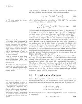
73. 58 Helium
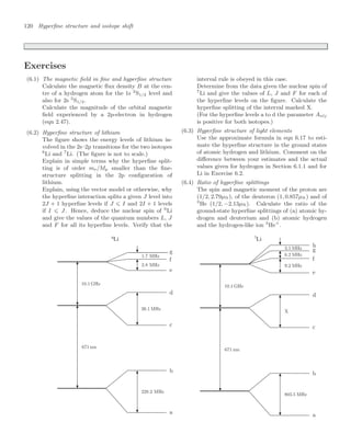
Exercises
More advanced problems are indicated by a *.
(3.1) Estimate of the binding energy of helium
(a) Write down the Schrödinger equation for the
helium atom and state the physical significance
of each of the terms.
(b) Estimate the equilibrium energy of an electron
bound to a charge +Ze by minimising
E(r) =
2
2mr2
−
Ze2
4π0r
.
(c) Calculate the repulsive energy between the two
electrons in helium assuming that r12 ∼ r.
Hence estimate the ionization energy of helium.
(d) Estimate the energy required to remove a fur-
ther electron from the helium-like ion Si12+
,
taking into account the scaling with Z of the
energy levels and the expectation value for
the electrostatic repulsion. The experimen-
tal value is 2400 eV. Compare the accuracy of
your estimates for Si12+
and helium. (IE(He)
= 24.6 eV.)
(3.2) Direct and exchange integrals for an arbitrary
system
(a) Verify that for
ψA
(r1, r2)
=
1
√
2
{uα(r1)uβ(r2) − uα(r2)uβ(r1) }
and H
= e2
/4π0r12 the expectation value
ψA
H
ψA
has the form J − K and give the
expressions for J and K.
(b) Write down the wavefunction ψS
that is orthog-
onal to ψA
.
(c) Verify that
ψA
H
ψS
= 0 so that H
is di-
agonal in this basis.
(3.3) Exchange integrals for a delta-function interaction
A particle in a square-well potential, with V (x) = 0
for 0 x and V (x) = ∞ elsewhere, has
normalised eigenfunctions u0(x) =
2/ sin (πx/ )
and u1(x) =
2/ sin (2πx/ ).
(a) What are the eigenenergies E0 and E1 of these
two wavefunctions for a particle of mass m?
(b) Two particles of the same mass m are both in
the ground state so that the energy of the whole
system is 2E0. Calculate the perturbation pro-
duced by a point-like interaction described by
the potential a δ (x1 − x2), with a constant.
(c) Show that, when the two interacting particles
occupy the ground and first excited states, the
direct and exchange integrals are equal. Also
show that the delta-function interaction pro-
duces no energy shift for the antisymmetric spa-
tial wavefunction and explain this in terms of
correlation of the particles. Calculate the en-
ergy of the other level of the perturbed system.
(d) For the two energy levels found in part (c),
sketch the spatial wavefunction as a function
of the coordinates of the two particles x1 and
x2. The particles move in one dimension but
the two-particle wavefunction exists in a two-
dimensional Hilbert space—draw either a con-
tour plot in the x1x2-plane or attempt a three-
dimensional sketch (by hand or computer).
(e) The two particles are identical and have spin
1/2. What is the total spin quantum number S
associated with each of the energy levels found
in part (c)?
∗(f) Discuss qualitatively the energy levels of this
system for two particles that have slightly dif-
ferent masses m1 = m2, so that they are distin-
guishable? [Hint. The spin has not been given
because it is not important for non-identical
particles.]
Comment. The antisymmetric spatial wavefunction
in part (c) clearly has different properties from a
straightforward product u0u1. The exchange inte-
gral is a manifestation of the entanglement of the
multiple-particle system.
(3.4) A helium-like system with non-identical particles
Imagine that there exists an exotic particle with the
same mass and charge as the electron but spin 3/2
(so it is not identical to the electron). This par-
ticle and an electron form a bound system with a
helium nucleus. Compare the energy levels of this
system with those of the helium atom. Describe
the energy levels of a system with two of the ex-

74. Exercises for Chapter 3 59
otic particles bound to a helium nucleus (and no
electrons). [Hint. It is not necessary to specify the
values of total spin associated with the levels.]
(3.5) The integrals in helium
(a) Show that the integral in eqn 3.24 gives the
value stated in eqn 3.7.
(b) Estimate the ground-state energy of helium us-
ing the variational principle. (The details of
this technique are not given in this book; see
the section on further reading.)
(3.6) Calculation of integrals for the 1s2p configuration
(a) Draw a scale diagram of RZ=2
1s (r), RZ=1
2s (r)
and RZ=1
2p (r). (See Table 2.2.)
(b) Calculate the direct integral in eqn 3.31 and
show that it gives
J1s2p = −
e2
/4π0
2a0
13
2 × 55
.
Give the numerical value in eV (cf. that given
in the text).
(3.7) Expansion of 1/r12
For r1 r2 the binomial expansion of
1
r12
=
r2
1 + r2
2 − 2r1r2 cos θ12
−1/2
is
1
r12
=
1
r2
1 − 2
r1
r2
cos θ12 +
r1
r2
2 −1/2
1
r2
1 +
r1
r2
cos θ12 + . . .
. (3.36)
(When r1 r2 we must interchange r1 and r2 to ob-
tain convergence.) The cosine of the angle between
r1 and r2 is
cos θ12 =
r1 ·
r2
= cos θ1 cos θ2 + sin θ1 sin θ2 cos (φ1 − φ2) .
(a) Show that the first two terms in the binomial
expansion agree with the terms with k = 0 and
1 in eqn 3.30.
(b) The repulsion between a 1s- and an nl-electron
is independent of m. Explain why, physically
or mathematically.
(c) Show that eqn 3.32 leads to eqn 3.34 for l = 1.
(d) For a 1snl configuration, the quantity K(r1, r2)
in eqn 3.34 is proportional to rl
1/rl+1
2 when
r1 r2. Explain this in terms of mathemat-
ical properties of the Yl,m functions.
Web site:
http://www.physics.ox.ac.uk/users/foot
This site has answers to some of the exercises, corrections and other supplementary information.

75. The alkalis
4
4.1 Shell structure and the
periodic table 60
4.2 The quantum defect 61
4.3 The central-field
approximation 64
4.4 Numerical solution of the
Schrödinger equation 68
4.5 The spin–orbit interaction:
a quantum mechanical
approach 71
4.6 Fine structure in the alkalis 73
Further reading 75
Exercises 76
4.1 Shell structure and the periodic table
For multi-electron atoms we cannot solve the Hamiltonian analytically,
but by making appropriate approximations we can explain their struc-
ture in a physically meaningful way. To do this, we start by considering
the elementary ideas of atomic structure underlying the periodic table
of the elements. In the ground states of atoms the electrons have the
configuration that minimises the energy of the whole system. The elec-
trons do not all fall down into the lowest orbital with n = 1 (the K-shell)
because the Pauli exclusion principle restricts the number of electrons
in a given (sub-)shell—two electrons cannot have the same set of quan-
tum numbers. This leads to the ‘building-up’ principle: electrons fill up
higher and higher shells as the atomic number Z increases across the
periodic table.1
Full shells are found at atomic numbers Z = 2, 10, . . .
1
Also referred to by its original German
name as the Aufbauprinciple. An ex-
tensive discussion of the atomic struc-
ture that underlies the periodic table
can be found in chemistry texts such as
Atkins (1994).
corresponding to helium and the other inert gases. These inert gases, in
a column on the right-hand side of the periodic table (see inside front
cover), were originally grouped together because of their similar chemical
properties, i.e. the difficulty in removing an electron from closed shells
means that they do not readily undergo chemical reactions.2
However,
2
Most of the arrangement of elements
in a periodic table was determined by
chemists, such as Mendeleev, in the
nineteenth century. A few inconsisten-
cies in the ordering were resolved by
Moseley’s measurements of X-ray spec-
tra (see Chapter 1).
inert gas atoms can be excited to higher-lying configurations by bom-
bardment with electrons in a gas discharge, and such processes are very
important in atomic and laser physics, as in the helium–neon laser.
The ground states of the alkalis have the following electronic con-
figurations:3
3
The configuration of an atom is spec-
ified by a list of nl with the occupancy
as an exponent. Generally, we do not
need to list the full configuration and it
is sufficient to say that a sodium atom
in its ground state has the configura-
tion 3s. A sodium ‘atom’ with one elec-
tron in the 3s level, and no others, is
an excited state of the highly-charged
ion Na+10—this esoteric system can be
produced in the laboratory but confu-
sion with the common sodium atom is
unlikely.
lithium Li 1s2
2s ,
sodium Na 1s2
2s2
2p6
3s ,
potassium K 1s2
2s2
2p6
3s2
3p6
4s ,
rubidium Rb 1s2
2s2
2p6
3s2
3p6
3d10
4s2
4p6
5s ,
caesium Cs 1s2
2s2
2p6
3s2
3p6
3d10
4s2
4p6
4d10
5s2
5p6
6s .
The alert reader will notice that the sub-shells of the heavier alkalis
are not filled in the same order as the hydrogenic energy levels, e.g. elec-
trons occupy the 4s level in potassium before the 3d level (for reasons
that emerge later in this chapter). Thus, strictly speaking, we should
say that the inert gases have full sub-shells, e.g. argon has the electronic

76. 4.2 The quantum defect 61
Table 4.1 Ionization energies of the inert gases and alkalis.
Element Z IE (eV)
He 2 24.6
Li 3 5.4
Ne 10 21.6
Na 11 5.1
Ar 18 15.8
K 19 4.3
Kr 36 14.0
Rb 37 4.2
Xe 54 12.1
Cs 55 3.9
configuration 1s2
2s2
2p6
3s2
3p6
with the 3d sub-shell unoccupied.4 4
This book takes a shell to be all energy
levels of the same principal quantum
number n, but the meaning of shell and
sub-shell may be different elsewhere.
We use sub-shell to denote all energy
levels with specific values of n and l
(in a shell with a given value of n).
We used these definitions in Chapter 1;
the inner atomic electrons involved in
X-ray transitions follow the hydrogenic
ordering.
Each alkali metal comes next to an inert gas in the periodic table
and much of the chemistry of the alkalis can be explained by the simple
picture of their atoms as having a single unpaired electron outside a core
of closed electronic sub-shells surrounding the nucleus. The unpaired
valence electron determines the chemical bonding properties; since it
takes less energy to remove this outer electron than to pull an electron
out of a closed sub-shell (see Table 4.1), thus the alkalis can form singly-
charged positive ions and are chemically reactive.5
However, we need
5
For a plot of the ionization energies of
all the elements see Grant and Phillips
(2001, Chapter 11, Fig. 18). This
figure is accessible at http://www.
oup.co.uk/best.textbooks/physics/
ephys/illustrations/.
more than this simple picture to explain the details of the spectra of the
alkalis and in the following we shall consider the wavefunctions.
4.2 The quantum defect
The energy of an electron in the potential proportional to 1/r depends
only on its principal quantum number n, e.g. in hydrogen the 3s, 3p and
3d configurations all have the same gross energy. These three levels are
not degenerate in sodium, or any atom with more than one electron,
and this section explains why. Figure 4.1 shows the probability density
of 3s-, 3p- and 3d-electrons in sodium. The wavefunctions in sodium
have a similar shape (number of nodes) to those in hydrogen. The 3d
wavefunction has a single lobe outside the core so that it experiences
almost the same potential as in a hydrogen atom; therefore this electron,
and other d configurations in sodium with n 3, have binding energies
similar to those in hydrogen, as shown in Fig. 4.2. In contrast, the
wavefunctions for the s-electrons have a significant value at small r—
they penetrate inside the core and ‘see’ more of the nuclear charge. Thus
the screening of the nuclear charge by the other electrons in the atom is
less effective for ns configurations than for nd, and s-electrons have lower
energy than d-electrons with the same principal quantum number. (The
np-electrons lie between these two.6
) The following modified form of
6
This dependence of the energy on the
quantum number l can also be ex-
plained in terms of the elliptical or-
bits of Bohr–Sommerfeld quantum the-
ory rather than Schrödinger’s wave-
functions; however, we shall use only
the ‘proper’ wavefunction description
since the detailed correspondence be-
tween the elliptical classical trajectories
and the radial wavefunctions can lead
to confusion.

77. 62 The alkalis
Fig. 4.1 The probability density of the
electrons in a sodium atom as a func-
tion of r. The electrons in the n = 1
and n = 2 shells make up the core,
and the probability density of the un-
paired outer electron is shown for the
n = 3 shell with l = 0, 1 and 2. The
probability is proportional to |P (r)|2 =
r2|R(r)|2; the r2 factor accounts for the
increase in volume of the spherical shell
between r and r + dr (i.e. 4πr2 dr) as
the radial distance increases. The de-
creasing penetration of the core as l
increases can be seen clearly—the 3d-
electron lies mostly outside the core
with a wavefunction and binding en-
ergy very similar to those for the 3d
configuration in hydrogen. These wave-
functions could be calculated by the
simple numerical method described in
Exercise 4.10, making the ‘frozen core’
approximation, i.e. that the distribu-
tion of the electrons in the core is
not affected by the outer electron—this
gives sufficient accuracy to illustrate
the qualitative features. (The iterative
method described in Section 4.4 could
be used to obtain more accurate numer-
ical wavefunctions.)
0
(b)
(a)
0
Core
Core
0
(c)
Core
Bohr’s formula works amazingly well for the energy levels of the alkalis:
E (n, l) = −hc
R∞
(n − δl)
2 . (4.1)
A quantity δl, called the quantum defect, is subtracted from the prin-
cipal quantum number to give an effective principal quantum number
n∗
= n − δl.7
The values of the quantum defects for each l can be esti-
7
This differs from the modification
used for X-ray transitions in Chapter
1—hardly surprising since the physical
situation is completely different for the
inner and outer electrons.
mated by inspecting the energy levels shown in Fig. 4.2. The d-electrons
have a very small quantum defect, δd 0, since their energies are nearly
hydrogenic. We can see that the 3p configuration in sodium has com-
parable energy to the n = 2 shell in hydrogen, and similarly for 4p and
n = 3, etc.; thus δp ∼ 1. It is also clear that the quantum defect for
s-electrons is greater than that for p-electrons. A more detailed analysis
shows that all the energy levels of sodium can be parametrised by the
above formula and only three quantum defects:

78. 4.2 The quantum defect 63
−1
−2
−3
−4
−5
−6
0
3
2
4
5
6
7
8
9
10
H
Sodium
Fig. 4.2 The energies of the s, p, d and
f configurations in sodium. The energy
levels of hydrogen are marked on the
right for comparison. The guidelines
link configurations with the same n to
show how the energies become closer to
the hydrogenic values as l increases, i.e.
the quantum defects decrease so that
δl 0 for f-electrons (and for the con-
figurations with l 3 that have not
been drawn).
δs = 1.35 , δp = 0.86 , δd = 0.01 , δl 0.00 for l 2 .
There is a small variation with n (see Exercise 4.3). Having examined
the variation in the quantum defects with orbital angular momentum
quantum number for a given element, now let us compare the quantum
defects in different alkalis. The data in Table 4.1 show that the alkalis
have similar ionization energies despite the variation in atomic number.
Thus the effective principal quantum numbers n∗
= (13.6 eV/IE)1/2

79. 64 The alkalis
Table 4.2 The effective principal quantum numbers and quantum defects for the
ground configuration of the alkalis. Note that the quantum defects do depend slightly
on n (see Exercise 4.3), so the value given in this table for the 3s-electron in sodium
differs slightly from the value given in the text (δs = 1.35) that applies for n 5.
Element Configuration n∗
δs
Li 2s 1.59 0.41
Na 3s 1.63 1.37
K 4s 1.77 2.23
Rb 5s 1.81 3.19
Cs 6s 1.87 4.13
(from eqn 4.1) are remarkably similar for all the ground configurations
of the alkalis, as shown in Table 4.2.
In potassium the lowering of the energy for the s-electrons leads to the
4s sub-shell filling before 3d. By caesium (spelt cesium in the US) the
6s configuration has lower energy than 4f (δf 0 for Cs). The exercises
give other examples, and quantum defects are tabulated in Kuhn (1969)
and Woodgate (1980), amongst others.
4.3 The central-field approximation
The previous section showed that the modification of Bohr’s formula by
the quantum defects gives reasonably accurate values for the energies
of the levels in alkalis. We described an alkali metal atom as a single
electron orbiting around a core with a net charge of +1e, i.e. the nucleus
surrounded by N − 1 electrons. This is a top-down approach where we
consider just the energy required to remove the valence electron from
the rest of the atom; this binding energy is equivalent to the ionization
energy of the atom. In this section we start from the bottom up and
consider the energy of all the electrons. The Hamiltonian for N electrons
in the Coulomb potential of a charge +Ze is
H =
N
i=1



−
2
2m
∇2
i −
Ze2
/4π0
ri
+
N
ji
e2
/4π0
rij



. (4.2)
The first two terms are the kinetic energy and potential energy for each
electron in the Coulomb field of a nucleus of charge Z. The term with
rij = |ri − rj| in the denominator is the electrostatic repulsion between
the two electrons at ri and rj. The sum is taken over all electrons with
j i to avoid double counting.8
This electrostatic repulsion is too large
8
For example, lithium has three inter-
actions between the three electrons, in-
versely proportional to r12, r13 and r23;
summing over all j for each value of i
would give six terms.
to be treated as a perturbation; indeed, at large distances the repulsion
cancels out most of the attraction to the nucleus. To proceed further
we make the physically reasonable assumption that a large part of the
repulsion between the electrons can be treated as a central potential

80. 4.3 The central-field approximation 65
S (r). This follows because the closed sub-shells within the core have
a spherical charge distribution, and therefore the interactions between
the different shells and between shells and the valence electron are also
spherically symmetric. In this central-field approximation the total po-
tential energy depends only on the radial coordinate:
VCF (r) = −
Ze2
/4π0
r
+ S(r) . (4.3)
In this approximation the Hamiltonian becomes
HCF =
N
i=1
−
2
2m
∇2
i + VCF (ri)
. (4.4)
For this form of potential, the Schrödinger equation for N electrons,
Hψ = Eatomψ, can be separated into N one-electron equations, i.e.
writing the total wavefunction as a product of single-electron wavefunc-
tions, namely
ψatom = ψ1ψ2ψ3 · · · ψN , (4.5)
leads to N equations of the form
−
2
2m
∇2
1 + VCF (r1)
ψ1 = E1ψ1 , (4.6)
and similar for electrons i = 2 to N. This assumes that all the elec-
trons see the same potential, which is not as obvious as it may appear.
This symmetric wavefunction is useful to start with (cf. the treatment
of helium before including the effects of exchange symmetry); however,
we know that the overall wavefunction for electrons, including spin,
should be antisymmetric with respect to an interchange of the particle
labels. (Proper antisymmetric wavefunctions are used in the Hartree–
Fock method mentioned later in this chapter.) The total energy of the
system is Eatom = E1 + E2 + . . . + EN . The Schrödinger equations for
each electron (eqn 4.6) can be separated into parts to give wavefunctions
of the form ψ1 = R(r1)Yl1,m1 ψspin(1). Angular momentum is conserved
in a central field and the angular equation gives the standard orbital
angular momentum wavefunctions, as in hydrogen. In the radial equa-
tion, however, we have VCF(r) rather than a potential proportional to
1/r and so the equation for P (r) = rR (r) is
−
2
2m
d2
dr2
+ VCF (r) +
2
l (l + 1)
2mr2
P(r) = EP(r) . (4.7)
To solve this equation we need to know the form of VCF(r) and compute
the wavefunctions numerically. However, we can learn a lot about the
behaviour of the system by thinking about the form of the solutions,
without actually getting bogged down in the technicalities of solving the
equations. At small distances the electrons experience the full nuclear
charge so that the central electric field is
E(r) →
Ze
4π0r2
r . (4.8)

81. 66 The alkalis
1
11
Fig. 4.3 The change-over from the short- to the long-range is not calculated but is
drawn to be a reasonable guess, using the following criteria. The typical radius of
the 1s wavefunction around the nucleus of charge +Ze = +11e is about a0/11, and
so Zeff will start to drop at this distance. We know that Zeff ∼ 1 at the distance
at which the 3d wavefunction has appreciable probability since that eigenstate has
nearly the same energy as in hydrogen. The form of the function Zeff (r) can be
found quantitatively by the Thomas–Fermi method described in Woodgate (1980).
At large distances the other N − 1 electrons screen most of the nuclear
charge so that the field is equivalent to that of charge +1e:
E(r) →
e
4π0r2
r . (4.9)
These two limits can be incorporated in a central field of the form
ECF(r) →
Zeffe
4π0r2
r . (4.10)
The effective atomic number Zeff (r) has limiting values of Zeff(0) = Z
and Zeff (r) → 1 as r → ∞, as sketched in Fig. 4.3.9
The potential
9
This is not necessarily the best way to
parametrise the problem for numerical
calculations but it is useful for under-
standing the underlying physical prin-
ciples.
energy of an electron in the central field is obtained by integrating from
infinity:
VCF(r) = e
r
∞
|ECF(r
)| dr
. (4.11)
The form of this potential is shown in Fig. 4.4.
So far, in our discussion of the sodium atom in terms of the wave-
function of the valence electron in a central field we have neglected
Fig. 4.4 The form of the potential en-
ergy of an electron in the central-field
approximation (e2
M = e2/4π0). This
approximate sketch for a sodium atom
shows that the potential energy crosses
over from VCF(r) = −e2
M/r at long
range to −11e2
M/r + Voffset; the con-
stant Voffset comes from the integration
in eqn 4.11 (if Zeff (r) = 11 for all r then
Voffset = 0 but this is not the case). For
electrons with l 0 the effective poten-
tial should also include the term that
arises from the angular momentum, as
shown in Fig. 4.5.

82. 4.3 The central-field approximation 67
Fig. 4.5 The total potential in the
central-field approximation including
the term that is proportional to l(l +
1)/r2 drawn here for l = 2 and the
same approximate electrostatic VCF(r)
as shown in Fig. 4.4. The angular
momentum leads to a ‘centrifugal bar-
rier’ that tends to keep the wavefunc-
tions of electrons with l 0 away from
r = 0 where the central-field potential
is deepest.
the fact that the central field itself depends on the configuration of the
electrons in the atom. For a more accurate description we must take
into account the effect of the outer electron on the other electrons, and
hence on the central field. The energy of the whole atom is the sum of
the energies of the individual electrons (in eqn 4.6), e.g. a sodium atom in
the 3s configuration has energy E
1s2
2s2
2p6
3s
= 2E1s +2E2s +6E2p +
E3s = Ecore +E3s. This is the energy of the neutral atom relative to the
bare nucleus (Na11+
).10
It is more useful to measure the binding energy 10
This is a crude approximation, espe-
cially for inner electrons.
relative to the singly-charged ion (Na+
) with energy E
1s2
2s2
2p6
=
2E
1s+2E
2s+6E
2p = E
core. The dashes are significant—the ten electrons
in the ion and the ten electrons in the core of the atom have slightly
different binding energies because the central field is not the same in
the two cases. The ionization energy is IE = Eatom − Eion = (Ecore −
E
core) + E3s. From the viewpoint of valence electrons, the difference
in Ecore between the neutral atom and the ion can be attributed to
core polarization, i.e. a change in the distribution of charge in the core
produced by the valence electron.11
To calculate the energy of multi-
11
This effect is small in the alkalis and
it is reasonable to use the frozen core
approximation that assumes Ecore
E
core. This approximation becomes
more accurate for a valence electron in
higher levels where the influence on the
core becomes smaller.

83. 68 The alkalis
electron atoms properly we should consider the energy of the whole
system rather than focusing attention on only the valence electron. For
example, neon has the ground configuration 1s2
2s2
2p6
and the electric
field changes significantly when an electron is excited out of the 2p sub-
shell, e.g. into the 1s2
2s2
2p5
3s configuration.
Quantum defects can be considered simply as empirical quantities that
happen to give a good way of parametrising the energies of the alkalis but
there is a physical reason for the form of eqn 4.1. In any potential that
tends to 1/r at long range the levels of bound states bunch together
as the energy increases—at the top of the well the classically allowed
region gets larger and so the intervals between the eigenenergies and the
stationary solutions get smaller.12
More quantitatively, in Exercise 1.12
12
This is in contrast to an infinite
square well where confinement to a re-
gion of fixed dimensions gives energies
proportional to n2, where n is an inte-
ger.
it was shown, using the correspondence principle, that such a potential
has energies E ∝ 1/k2
, with ∆k = 1 between energy levels, but k
is not itself necessarily an integer. For the special case of a potential
proportional to 1/r for all distances, k is an integer that we call the
principal quantum number n and the lowest energy level turns out to
be n = 1. For a general potential in the central-field approximation we
have seen that it is convenient to write k in terms of the integer n as
k = n−δ, where δ is a non-integer (quantum defect). To find the actual
energy levels of an alkali and hence δ (for a given value of l) requires the
numerical calculation of the wavefunctions, as outlined in the following
section.
4.4 Numerical solution of the Schrödinger
equation
Before describing particular methods of solution, let us look at the gen-
eral features of the wavefunction for particles in potential wells. The
radial equation for P (r) has the form
d2
P
dr2
= −
2m
2
{E − V (r)} P , (4.12)
where the potential V (r) includes the angular momentum term in eqn
4.7. Classically, the particle is confined to the region where E−V (r) 0
since the kinetic energy must be positive. The positions where E = V (r)
are the classical turning points where the particle instantaneously comes
to rest, cf. at the ends of the swing of a pendulum. The quantum
wavefunctions are oscillatory in the classically allowed region, with the
curvature and number of nodes both increasing as E − V (r) increases,
as shown in Fig. 4.6. The wavefunctions penetrate some way into the
classically forbidden region where E − V (r) 0; but in this region the
solutions decay exponentially and the probability falls off rapidly.
How can we find P (r) in eqn 4.12 without knowing the potential V (r)?
The answer is firstly to find the wavefunctions for a potential VCF(r)
that is ‘a reasonable guess’, consistent with eqn 4.11 and the limits on
the central electric field in the previous equations. Then, secondly, we

84. 4.4 Numerical solution of the Schrödinger equation 69
50 100
Arbitrary
units
Fig. 4.6 The potential in the central-
field approximation including the term
that is proportional to l(l + 1)/r2 is
drawn here for l = 2 and the same
approximate electrostatic VCF(r) as
shown in Fig. 4.4. The function P (r) =
rR(r) was drawn for n = 6 and l = 2
using the method described in Exer-
cise 4.10.
make the assumed potential correspond closely to the real potential, as
described in the next section. Equation 4.12 is a second-order differen-
tial equation and we can numerically calculate P (r), the value of the
function at r, from two nearby values, e.g. u (r − δr) and u (r − 2δr).13 13
The step size δr must be small com-
pared to the distance over which the
wavefunction varies; but the number of
steps must not be so large that round-
off errors begin to dominate.
Thus, working from near r = 0, the method gives the numerical value of
the function at all points going out as far as is necessary. The region of
the calculation needs to extend beyond the classical turning point(s) by
an amount that depends on the energy of the wavefunction being calcu-
lated. These general features are clearly seen in the plots produced in
Exercise 4.10. Actually, that exercise describes a method of finding the
radial wavefunction R(r) rather than P (r) = rR (r) but similar princi-
ples apply.14
If you carry out the exercise you will find that the behaviour 14
In a numerical method there is no
reason why we should not calculate the
wavefunction directly; P (r) was intro-
duced to make the equations neater in
the analytical approach.
at large r depends very sensitively on the energy E—the wavefunction
diverges if E is not an eigenenergy of the potential—this gives a way
of searching for those eigenenergies. If the wavefunction diverges up-
wards for E
and downwards for E
then we know that an eigenenergy
of the system Ek lies between these two values, E
Ek E
. Test-
ing further values between these upper and lower bounds narrows the
range and gives a more precise value of Ek (as in the Newton–Raphson
method for finding roots). This so-called ‘shooting’ method is the least
sophisticated method of computing wavefunctions and energies, but it
is adequate for illustrating the principles of such calculations. Results
are not given here since they can readily be calculated—the reader is
strongly encouraged to implement the numerical method of solution, us-
ing a spreadsheet program, as described in Exercise 4.10. This shows
how to find the wavefunctions for an electron in an arbitrary potential
and verifies that the energy levels obey a quantum defect formula such
as eqn 4.1 in any potential that is proportional to 1/r at long range (see
Fig. 4.7).

85. 70 The alkalis
Fig. 4.7 Simple modifications of the
potential energy that could be used
for the numerical solution of the
Schrödinger equation described in Ex-
ercise 4.10. For all these potentials
V (r) = −e2/4π0r for r ⩾ rcore. (a)
Inside the radial distance rcore the po-
tential energy is V (r) = −Ze2/4π0r +
Voffset, drawn here for Z = 3 and an
offset chosen so that V (r) is continuous
at r = rcore. This corresponds to the
situation where the charge of the core is
an infinitely thin shell. The deep poten-
tial in the inner region means that the
wavefunction has a high curvature, so
small steps must be used in the numeri-
cal calculation (in this region). The hy-
pothetical potentials in (b) and (c) are
useful for testing the numerical method
and for showing why the eigenenergies
of any potential proportional to 1/r at
long range obey a quantum defect for-
mula (like eqn 4.1). The form of the
solution depends sensitively on the en-
ergy in the outer region r ⩾ rcore, but
in the inner region where |E| |V (r)|
it does not, e.g. the number of nodes
(‘wiggles’) in this region changes slowly
with energy E. Thus, broadly speak-
ing, the problem reduces to finding the
wavefunction in the outer region that
matches boundary conditions, at r =
rcore, that are almost independent of
the energy—the potential energy curve
shown in (b) is an extreme example
that gives useful insight into the be-
haviour of the wavefunction for more
realistic central fields.
0
0
(b)
(c)
(a)
4.4.1 Self-consistent solutions
The numerical method described above, or a more sophisticated one,
can be used to find the wavefunctions and energies for a given potential
in the central-field approximation. Now we shall think about how to de-
termine VCF itself. The potential of the central field in eqn 4.2 includes
the electrostatic repulsion of the electrons. To calculate this mutual
repulsion we need to know where the electrons are, i.e. their wavefunc-
tions, but to find the wavefunctions we need to know the potential. This
argument is circular. However, going round and round this loop can be
useful in the following sense. As stated above, the method starts by
making a reasonable estimate of VCF and then computing the electronic
wavefunctions for this potential. These wavefunctions are then used to
calculate a new average potential (using the central-field approximation)
that is more realistic than the initial guess. This improved potential is
then used to calculate more accurate wavefunctions, and so on. On suc-

86. 4.5 The spin–orbit interaction: a quantum mechanical approach 71
cessive iterations, the changes in the potential and wavefunctions should
get smaller and converge to a self-consistent solution, i.e. where the wave-
functions give a certain VCF(r), and solving the radial equation for that
central potential gives back the same wavefunctions (within the required
precision).15
This self-consistent method was devised by Hartree. How- 15
The number of iterations required,
before the changes when going round
the loop become very small, depends
on how well the initial potential is cho-
sen, but the final self-consistent solu-
tion should not depend on the initial
choice. In general, it is better to let a
computer do the work rather than ex-
pend a lot of effort improving the start-
ing point.
ever, the wavefunctions of multi-electron atoms are not simply products
of individual wavefunctions as in eqn 4.5. In our treatment of the excited
configurations of helium we found that the two-electron wavefunctions
had to be antisymmetric with respect to the permutation of the electron
labels. This symmetry requirement for identical fermions was met by
constructing symmetrised wavefunctions that were linear combinations
of the simple product states (i.e. the spatial part of these functions is
ψA
space and ψS
space). A convenient way to extend this symmetrisation to
N particles is to write the wavefunction as a Slater determinant:
Ψ =
1
√
N
ψa (1) ψa (2) · · · ψa (N)
ψb (1) ψb (2) · · · ψb (N)
ψc (1) ψc (2) · · · ψc (N)
.
.
.
.
.
.
...
.
.
.
ψx (1) ψx (2) · · · ψx (N)
.
Here a, b, c, . . . , x are the possible sets of quantum numbers of the in-
dividual electrons,16
and 1, 2, . . . , N are the electron labels. The change 16
Including both space and spin.
of sign of a determinant on the interchange of two columns makes the
wavefunction antisymmetric. The Hartree–Fock method uses such sym-
metrised wavefunctions for self-consistent calculations and nowadays this
is the standard way of computing wavefunctions, as described in Brans-
den and Joachain (2003). In practice, numerical methods need to be
adapted to the particular problem being considered, e.g. numerical val-
ues of the radial wavefunctions that give accurate energies may not give
a good value for a quantity such as the expectation value
1/r3
that is
very sensitive to the behaviour at short range.
4.5 The spin–orbit interaction: a quantum
mechanical approach
The spin–orbit interaction βs · l (see eqn 2.49) splits the energy levels to
give fine structure. For the single valence in an alkali we could treat this
interaction in exactly the same way as for hydrogen in Chapter 2, i.e. use
the vector model that treats the angular momenta as vectors obeying
classical mechanics (supplemented with rules such as the restriction of
the angular momentum to integer or half-integer values). However, in
this chapter we shall use a quantum mechanical treatment and regard the
vector model as a useful physical picture that illustrates the behaviour
of the quantum mechanical operators. The previous discussion of fine
structure in terms of the vector model had two steps that require further
justification.

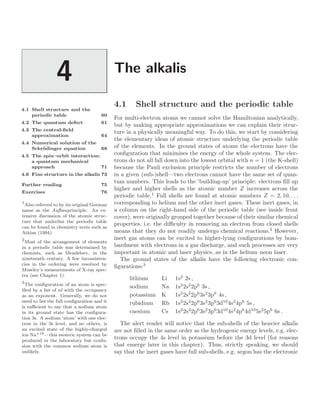
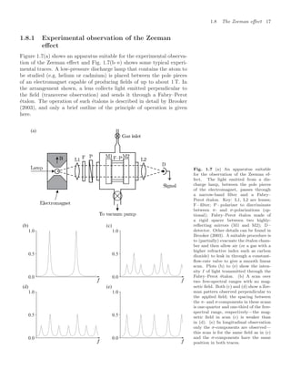
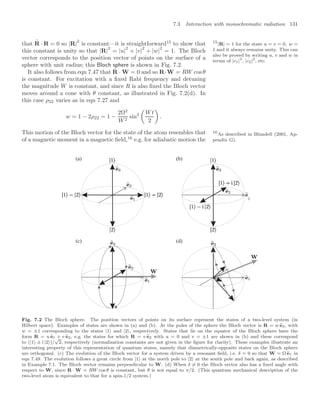
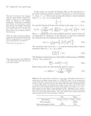
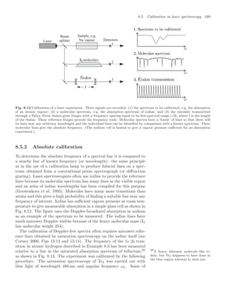
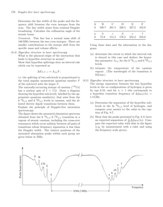
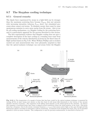
87. 72 The alkalis
(a) The possible values of the total angular momentum obtained by
the addition of the electron’s spin, s = 1/2, and its orbital angular
momentum are j = l + 1/2 or l − 1/2. This is a consequence of the
rules for the addition of angular momentum in quantum mechanics
(vector addition but with the resultant quantised).
(b) The vectors have squared magnitudes given by j2
= j(j + 1), l2
=
l(l + 1) and s2
= 3/4, where j and l are the relevant angular mo-
mentum quantum numbers.
Step (b) arises from taking the expectation values of the quantum op-
erators in the Hamiltonian for the spin–orbit interaction. This is not
straightforward since the atomic wavefunctions R(r) |l ml s ms are not
eigenstates of this operator17
—this means that we must face the com-
17
The wavefunction for an alkali metal
atom in the central-field approxima-
tion is a product of a radial wavefunc-
tion (which does not have an analyti-
cal expression) and angular momentum
eigenfunctions (as in hydrogen).
plications of degenerate perturbation theory. This situation arises fre-
quently in atomic physics and merits a careful discussion.
We wish to determine the effect of an interaction of the form s · l
on the angular eigenfunctions |l ml s ms . These are eigenstates of the
operators l2
, lz, s2
and sz labelled by the respective eigenvalues.18
There
18
More explicitly, we have
|l ml s ms ≡ Yl,ml
ψspin, where
ψspin = |ms = +1/2 or |ms = −1/2.
are 2(2l+1) degenerate eigenstates for each value of l because the energy
does not depend on the orientation of the atom in space, or the direction
of its spin, i.e. energy is independent of ml and ms. The states |l ml s ms
are not eigenstates of s · l because this operator does not commute with
lz and sz: [s · l, lz] = 0 and [s · l, sz] = 0.19
Quantum operators only
19
Proof of these commutation re-
lations: [sxlx + syly + szlz, lz] =
sx [lx, lz]+sy [ly, lz] = −isxly +isylx =
0. Similarly, [sxlx + syly + szlz, sz] =
−isylx + isxly = 0. Note that
[s · l, lz] = − [s · l, sz] and hence s · l
commutes with lz + sz.
have simultaneous eigenfunctions if they commute. Since |l ml s ms is
an eigenstate of lz it cannot simultaneously be an eigenstate of s · l, and
similarly for sz. However, s·l does commute with l2
and s2
:
!
s · l, l2
= 0
and
!
s · l, s2
= 0 (which are easy to prove since sx, sy, sz, lx, ly and
lz all commute with s2
and l2
). So l and s are good quantum numbers
in fine structure. Good quantum numbers correspond to constants of
motion in classical mechanics—the magnitudes of l and s are constant
but the orientations of these vectors change because of their mutual
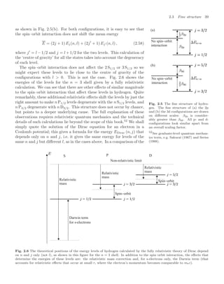
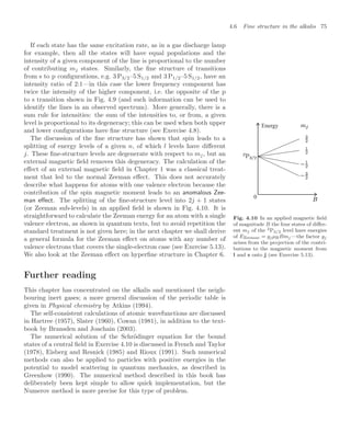
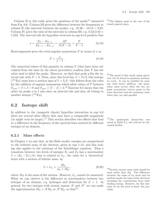
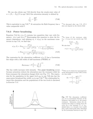
interaction, as shown in Fig. 4.8. If we try to evaluate the expectation
value using wavefunctions that are not eigenstates of the operator then
things get complicated. We would find that the wavefunctions are mixed
by the perturbation, i.e. in the matrix formulation of quantum mechanics
the matrix representing the spin–orbit interaction in this basis has off-
diagonal elements. The matrix could be diagonalised by following the
standard procedure for finding the eigenvalues and eigenvectors,20
but
20
As for helium in Section 3.2 and in
the classical treatment of the normal
Zeeman effect in Section 1.8.
a p-electron gives six degenerate states so the direct approach would
require the diagonalisation of a 6×6 matrix. It is much better to find the
eigenfunctions at the outset and work in the appropriate eigenbasis. This
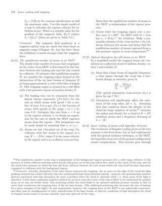
‘look-before-you-leap’ approach requires some preliminary reasoning.
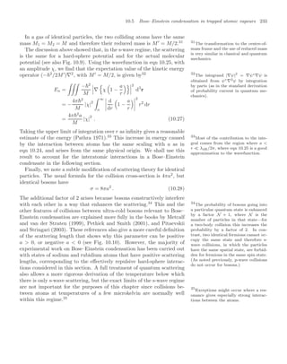
l
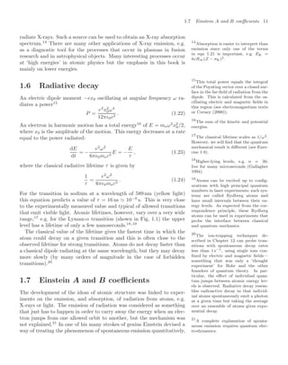
s
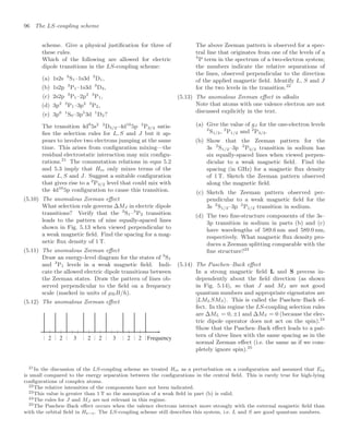
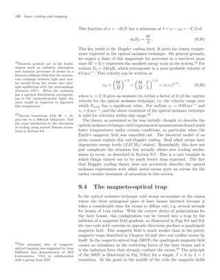
j
Fig. 4.8 The total angular momen-
tum of the atom j = l + s is a fixed
quantity in the absence of an exter-
nal torque. Thus an interaction be-
tween the spin and orbital angular mo-
menta βs · l causes these vectors to ro-
tate (precess) around the direction of j
as shown.
We define the operator for the total angular momentum as j = l + s.
The operator j2
commutes with the interaction, as does its component
jz:
!
s · l, j2
= 0 and [s · l, jz] = 0. Thus j and mj are good quantum
numbers.21
Hence suitable eigenstates for calculating the expectation
21
These commutation relations for the
operators correspond to the conserva-
tion of the total angular momentum,
and its component along the z-axis.
Only an external torque on the atom
affects these quantities. The spin–orbit
interaction is an internal interaction.
value of s · l are |l s j mj . Mathematically these new eigenfunctions can
be expressed as combinations of the old basis set:

88. 4.6 Fine structure in the alkalis 73
|lsjmj =
ml,ms
C(lsjmj; ml, ms) |l ml s ms .
Each eigenfunction labelled by l, s, j and mj is a linear combination of
the eigenfunctions with the same values of l and s but various values
of ml and ms. The coefficients C are the Clebsch–Gordan coefficients
and their values for many possible combinations of angular momenta
are tabulated in more advanced books. Particular values of Clebsch–
Gordan coefficients are not needed for the problems in this book but
it is important to know that, in principle, one set of functions can be
expressed in terms of another complete set—with the same number of
eigenfunctions in each basis.
Finally, we use the identity22
j2
= l2
+ s2
+ 2s · l to express the 22
This applies both for vector opera-
tors, where j2 = jx
2 + jy
2 + jz
2, and
for classical vectors where this is simply
j2 = |j|2.
expectation value of the spin–orbit interaction as
lsjmj| s · l |lsjmj = 1
2 lsjmj| j2
− l2
− s2
|lsjmj
= 1
2 {j(j + 1) − l (l + 1) − s (s + 1)} .
The states |lsjmj are eigenstates of the operators j2
, l2
and s2
. The
importance of the proper quantum treatment may not yet be apparent
since all we appear to have gained over the vector model is being able to
write the wavefunctions symbolically as |lsjmj . We will, however, need
the proper quantum treatment when we consider further interactions
that perturb these wavefunctions.
4.6 Fine structure in the alkalis
The fine structure in the alkalis is well approximated by an empirical
modification of eqn 2.56 called the Landé formula:
∆EFS =
Z2
i Z2
o
(n∗)
3
l (l + 1)
α2
hcR∞ . (4.13)
In the denominator the effective principal quantum number cubed (n∗
)
3
(defined in Section 4.2) replaces n3
. The effective atomic number Zeff,
which was defined in the discussion of the central-field approximation,
tends to the inner atomic number Zi ∼ Z as r → 0 (where the electron
‘sees’ most of the nuclear charge); outside the core the field corresponds
to an outer atomic number Zo 1 (for neutral atoms). The Landé
formula can be justified by seeing how the central-field approximation
modifies the calculation of the fine structure in hydrogen (Section 2.3.2).
The spin–orbit interaction depends on the electric field that the electron
moves through; in an alkali metal atom this field is proportional to
Zeff(r)r/r3
rather than r/r3
as in hydrogen.23
Thus the expectation 23
This modification is equivalent to us-
ing VCF in place of the hydrogenic po-
tential proportional to 1/r.
value of the spin–orbit interaction depends on
Zeff (r)
r3
≡
1
er
∂VCF (r)
∂r

89. 74 The alkalis
rather than
1/r3
as in hydrogen (eqn 2.51). This results in fine struc-
ture for the alkalis, given by the Landé formula, that scales as Z2
—this
lies between the dependence on Z4
for hydrogenic ions (no screening)
and the other extreme of no dependence on atomic number for complete
screening. The effective principal quantum number n∗
is remarkably
similar across the alkalis, as noted in Section 4.2.
As a particular numerical example of the scaling, consider the fine
structure of sodium (Z = 11) and of caesium (Z = 55). The 3p con-
figuration of sodium has a fine-structure splitting of 1700 m−1
, so for
a Z2
-dependence the fine structure of the 6p configuration of caesium
should be (using n∗
from Table 4.2)
1.7 × 103
×
55
11
2
×
2.1
2.4
3
= 28.5 × 103
m−1
.
This estimate gives only half the actual value of 55.4 × 103
m−1
, but
the prediction is much better than if we had used a Z4
scaling. (A
logarithmic plot of the energies of the gross and fine structure against
atomic number is given in Fig. 5.7. This shows that the actual trend of
the fine structure lies close to the Z2
-dependence predicted.)
The fine structure causes the familiar yellow line in sodium to be a
doublet comprised of the two wavelengths λ = 589.0 nm and 589.6 nm.
This, and other doublets in the emission spectrum of sodium, can be
resolved by a standard spectrograph. In caesium the transitions be-
tween the lowest energy configurations (6s–6p) give spectral lines at
λ = 852 nm and 894 nm—this ‘fine structure’ is not very fine.
4.6.1 Relative intensities of fine-structure
transitions
Frequency
Fig. 4.9 The fine-structure compo-
nents of a p to s transition, e.g. the
3 S1/2–3 P1/2 and 3 S1/2–3 P3/2 transi-
tions in sodium. (Not to scale.) The
statistical weights of the upper levels
lead to a 1:2 intensity ratio.
The transitions between the fine-structure levels of the alkalis obey the
same selection rules as in hydrogen since the angular momentum func-
tions are the same in both cases. It takes a considerable amount of cal-
culation to find absolute values of the transition rates24
but we can find
24
The rates of the allowed transitions
depend on integrals involving the radial
wavefunctions (carried out numerically
for the alkalis) and the integrals over
the angular part of the wavefunction
given in Section 2.2.1, where we derived
the selection rules.
the relative intensities of the transitions between different fine-structure
levels from a simple physical argument. As an example we shall look
at p to s transitions in sodium, as shown in Fig. 4.9. The 3 S1/2–3 P1/2
transition has half the intensity of the 3 S1/2–3 P3/2 transition.25
This
25
This shortened form of the full LS-
coupling scheme notation gives all the
necessary information for a single elec-
tron, cf. 3s 2S1/2–3p 2P3/2.
1:2 intensity ratio arises because the strength of each component is pro-
portional to the statistical weight of the levels (2j + 1). This gives 2:4
for j = 1/2 and 3/2. To explain this we first consider the situation
without fine structure. For the 3p configuration the wavefunctions have
the form R3p(r) |lmlsms and the decay rate of these states (to 3s) is
independent of the values of ml and ms.26
Linear combinations of the
26
This must be true for the physical
reason that the decay rate is the same
whatever the spatial orientation of the
atom, and similarly for the spin states.
All the different angular states have the
same radial integral, i.e. that between
the 3p and 3s radial wavefunctions.
states R(r) |lmlsms with different values of ml and ms (but the same
values of n, l and s, and hence the same lifetime) make up the eigen-
states of the fine structure, |lsjmj . Therefore an alkali atom has the
same lifetime for both values of j.27
27
This normal situation for fine struc-
ture may be modified slightly in a case
like caesium where the large separa-
tion of the components means that the
frequency dependence of the lifetime
(eqn 1.24) leads to differences, even
though the matrix elements are similar.

90. 4.6 Fine structure in the alkalis 75
If each state has the same excitation rate, as in a gas discharge lamp
for example, then all the states will have equal populations and the
intensity of a given component of the line is proportional to the number
of contributing mj states. Similarly, the fine structure of transitions
from s to p configurations, e.g. 3 P3/2–5 S1/2 and 3 P1/2–5 S1/2, have an
intensity ratio of 2:1—in this case the lower frequency component has
twice the intensity of the higher component, i.e. the opposite of the p
to s transition shown in Fig. 4.9 (and such information can be used to
identify the lines in an observed spectrum). More generally, there is a
sum rule for intensities: the sum of the intensities to, or from, a given
level is proportional to its degeneracy; this can be used when both upper
and lower configurations have fine structure (see Exercise 4.8).
The discussion of the fine structure has shown that spin leads to a
splitting of energy levels of a given n, of which l levels have different
j. These fine-structure levels are degenerate with respect to mj, but an
external magnetic field removes this degeneracy. The calculation of the
effect of an external magnetic field in Chapter 1 was a classical treat-
ment that led to the normal Zeeman effect. This does not accurately
describe what happens for atoms with one valence electron because the
contribution of the spin magnetic moment leads to an anomalous Zee-
man effect. The splitting of the fine-structure level into 2j + 1 states
(or Zeeman sub-levels) in an applied field is shown in Fig. 4.10. It is
straightforward to calculate the Zeeman energy for an atom with a single
valence electron, as shown in quantum texts, but to avoid repetition the
standard treatment is not given here; in the next chapter we shall derive
a general formula for the Zeeman effect on atoms with any number of
valence electrons that covers the single-electron case (see Exercise 5.13).
We also look at the Zeeman effect on hyperfine structure in Chapter 6.
Energy
0
Fig. 4.10 In an applied magnetic field
of magnitude B the four states of differ-
ent mj of the 2P3/2 level have energies
of EZeeman = gjµBBmj —the factor gj
arises from the projection of the contri-
butions to the magnetic moment from
l and s onto j (see Exercise 5.13).
Further reading
This chapter has concentrated on the alkalis and mentioned the neigh-
bouring inert gases; a more general discussion of the periodic table is
given in Physical chemistry by Atkins (1994).
The self-consistent calculations of atomic wavefunctions are discussed
in Hartree (1957), Slater (1960), Cowan (1981), in addition to the text-
book by Bransden and Joachain (2003).
The numerical solution of the Schrödinger equation for the bound
states of a central field in Exercise 4.10 is discussed in French and Taylor
(1978), Eisberg and Resnick (1985) and Rioux (1991). Such numerical
methods can also be applied to particles with positive energies in the
potential to model scattering in quantum mechanics, as described in
Greenhow (1990). The numerical method described in this book has
deliberately been kept simple to allow quick implementation, but the
Numerov method is more precise for this type of problem.

91. 76 The alkalis
Exercises
(4.1) Configuration of the electrons in francium
Write down the full electronic configuration of
francium (atomic number Z = 87). This element
comes below caesium in the periodic table.
(4.2) Finding the series limit for sodium
Eight ultraviolet absorption lines in sodium have
wavenumbers of
38 541 , 39 299 , 39 795 , 40 137 ,
40 383 , 40 566 , 40 706 , 40 814 ,
in units of cm−1
. Devise an extrapolation proce-
dure to find the ionization limit of sodium with a
precision justified by the data. Convert the result
into electron volts. (You may find a spreadsheet
program useful for manipulating the numbers.)
What is the effective principal quantum number
n∗
of the valence electron in the ground configu-
ration?
(4.3) Quantum defects of sodium
The binding energies of the 3s, 4s, 5s and 6s con-
figurations in sodium are 5.14 eV, 1.92 eV, 1.01 eV
and 0.63 eV, respectively. Calculate the quantum
defects for these configurations and comment on
what you find.
Estimate the binding energy of the 8s configura-
tion and make a comparison with the n = 8 shell
in hydrogen.
(4.4) Quantum defect
Estimate the wavelength of laser radiation that ex-
cites the 5s 2
S1/2–7s 2
S1/2 transition in rubidium
by simultaneous absorption of two photons with
the same frequency (IE(Rb) = 4.17 eV). (Two-
photon spectroscopy is described in Section 8.4 but
specific details are not required here.)
(4.5) Application of quantum defects to helium and
helium-like ions
Configuration Binding energy (cm−1
)
1s2s 35 250
1s2p 28 206
1s3s 14 266
1s3p 12 430
1s3d 12 214
(a) Calculate the wavelength of the 1s2p–1s3d line
in helium and compare it with the Balmer-α
line in hydrogen.
(b) Calculate the quantum defects for the config-
urations of helium in the table. Estimate the
binding energies of the 1s4l configurations.
(c) The levels belonging to the 1s4f configuration
of the Li+
ion all lie at an energy of 72.24 eV
above the ion’s ground state. Estimate the
second ionization energy of this ion. Answer:
75.64 eV.
(4.6) Quantum defects and fine structure of potassium
An atomic vapour of potassium absorbs light at
the wavelengths (in nm): 769.9, 766.5, 404.7,
404.4, 344.7 and 344.6. These correspond to the
transitions from the ground configuration 4s. Ex-
plain these observations as fully as you can and
estimate the mean wavelength of the next doublet
in the series, and its splitting. (Potassium has
IE = 4.34 eV.)28
(4.7) The Z-scaling of fine structure
Calculate the fine-structure splitting of the 3p con-
figuration of the hydrogen-like ion Na+10
(in eV).
Explain why it is larger than the fine structure
of the same configuration in the neutral sodium
(0.002 eV) and hydrogen (1.3 × 10−5
eV).
(4.8) Relative intensities of fine-structure components
(a) An emission line in the spectrum of an al-
kali has three fine-structure components cor-
responding to the transitions 2
P3/2–2
D3/2,
2
P3/2–2
D5/2 and 2
P1/2–2
D3/2. These compo-
nents have intensities a, b and c, respectively,
that are in the ratio 1 : 9 : 5. Show that these
satisfy the rule that the sum of the intensities
of the transitions to, or from, a given level is
proportional to its statistical weight (2J + 1).
(b) Sketch an energy-level diagram of the fine-
structure levels of the two terms nd 2
D and
n
f 2
F (for n
n). Mark the three allowed
electric dipole transitions and find their rela-
tive intensities.
28For a discussion of how to determine the quantum defect for a series of lines by an iterative method see Softley (1994).

92. Exercises for Chapter 4 77
(4.9) Spherical symmetry of a full sub-shell
The sum
#l
m=−l |Yl,m|2
is spherically symmetric.
Show this for the specific case of l = 1 and com-
ment on the relevance of the general expression,
that is true for all values of l, to the central-field
approximation.
(4.10) Numerical solution of the Schrödinger equation
This exercise goes through a method of finding the
wavefunctions and their energies for a potential (in
the central-field approximation). This shows how
numerical calculations are carried out in a simple
case that can be implemented easily on a computer
with readily available spreadsheet programs.29
Of
course, the properties of hydrogen-like atoms are
well known and so the first stage really serves
as a way of testing the numerical method (and
checking that the formulae have been typed cor-
rectly). It is straightforward to extend the nu-
merical method to deal with other cases, e.g. the
potentials in the central-field approximation illus-
trated in Fig. 4.7.30
(a) Derivation of the equations
Show from eqn 2.4, and other equations in
Chapter 2, that
d2
R
dx2
+
2
x
dR
dx
+
$
%
E − %
V (x)
R (x) = 0 , (4.14)
where the position and energy have been
turned into dimensionless variables: x = r/a0
and %
E is the energy in units of e2
/8π0a0 =
13.6 eV (equal to half the atomic unit of en-
ergy used in some of the references).31
In
these units the effective potential is
%
V (x) =
l (l + 1)
x2
−
2
x
, (4.15)
where l is the orbital angular momentum
quantum number.
The derivatives of a function f (x) can be ap-
proximated by
df
dx
=
f (x + δ/2) + f (x − δ/2)
δ
,
d2
f
dx2
=
f (x + δ) + f (x − δ) − 2f (x)
δ2
,
where δ is a small step size.32
Show that the second derivative follows by ap-
plying the procedure used to obtain the first
derivative twice. Show also that substitution
into eqn 4.14 gives the following expression for
the value of the function at x + δ in terms of
its value at the two previous points:
R(x + δ) =
2R(x) +
$
%
V (x) − %
E
R(x)δ2
−
1 −
δ
x
R(x − δ)
'
1 +
δ
x
.
(4.16)
If we start the calculation near the origin then
R (2δ) =
1
2
(
2 +
$
%
V (δ) − %
E
δ2
)
R (δ) ,
R (3δ) =
1
3
(
2R (2δ) +
$
%
V (2δ) − %
E
R (2δ) δ2
+ R (δ)
)
,
etc. Note that in the first equation the value of
R (x) at x = 2δ depends only on R (δ)—it can
easily be seen why by inspection of eqn 4.16
for the case of x = δ (for this value of x the
coefficient of R (0) is zero). Thus the calcula-
tion starts at x = δ and works outwards from
there.33
At all other positions (x δ) the
value of the function depends on its values at
the two preceding points. From these recur-
sion relations we can calculate the function at
all subsequent points.
The calculated functions will not be nor-
malised and the starting conditions can be
multiplied by an arbitrary constant without
affecting the eigenenergies, as will become
clear from looking at the results. In the fol-
lowing R (δ) = 1 is the suggested choice but
any starting value works.
(b) Implementation of the numerical method
using a spreadsheet program
Follow these instructions.
1. Type the given text labels into cells A1, B1,
C1, D2, E2 and F2 and the three numbers
into cells D1, E1 and F1 so that it has the
following form:
29With a spreadsheet it is very easy to make changes, e.g. to find out how different potentials affect the eigenenergies and
wavefunctions.
30It is intended to put more details on the web site associated with this book, see introduction for the address.
31The electron mass me = 1 in these units. Or, more strictly, its reduced mass.
32This abbreviation should not be confused with the quantum defect.
33This example is an exception to the general requirement that the solution of a second-order differential equation, such as
that for a harmonic oscillator, requires a knowledge of the function at two points to define both the value of the function and
its derivative.

93. 78 The alkalis
A B C D E F
1 x V(x) psi 0.02 −0.25 1
2 step energy ang.mom.
Column A will contain the x-coordinates,
the potential will be in column B and the
function in column C. Cells D1, E1 and F1
contain the step size, energy and orbital an-
gular momentum quantum number (l = 1),
respectively.
2. Put 0 into A2 and the formula =A2+$D$1
into A3. Copy cell A3 to the block
A4:A1002. (Or start with a smaller num-
ber of steps and adjust D1 accordingly.)
3. The potential diverges at x = 0 so type
inf. into B2 (or leave it blank, remember-
ing not to refer to it).
Put the formula
=-2/A3 +$F$1*($F$1+1)/(A3*A3)
into cell B3 (as in eqn 4.15). Copy B3 into
the block B4:B1002.
4. This is the crucial stage that calculates
the function. Type the number 1 into cell
C3. (We leave C2 blank since, as explained
above, the value of the function at x = 0
does not affect the solution given by the re-
cursion relation in eqn 4.16.) Now move to
cell C4 and enter the following formula for
the recursion relation:
=( 2*C3+(B3-$E$1)*C3*$D$1*$D$1
- (1-$D$1/A3)*C2 )/ (1+$D$1/A3).
Copy this into the block C5:C1002. Create
an xy-plot of the wavefunction (with data
points connected by smooth lines and no
markers); the x series is A2:A1002 and the
y series is C2:C1002. Insert this graph on
the sheet.
5. Now play around with the parameters and
observe the effect on the wavefunction for
a particular energy.
(i) Show that the initial value of the func-
tion does not affect its shape, or the
eigenenergy, by putting 0.1 (or any
number) into cell C3.
(ii) Change the energy, e.g. put -0.251
into cell E1, then -0.249, and ob-
serve the change in behaviour at large
x. (The divergence is exponential, so
even a small energy discrepancy gives
a large effect.) Try the different ener-
gies again with bigger and smaller step
sizes in D1. It is important to search
for the eigenenergy using an appropri-
ate range of x. The eigenenergy lies
between the two values of the trial en-
ergy that give opposite divergence, i.e.
upwards and downwards on the graph.
(iii) Change F1 to 0 and find a solution for
l = 0.
6. Produce a set of graphs labelled clearly
with the trial energy that illustrate the
principles of the numerical solution, for the
two functions with n = 2 and two other
cases. Compare the eigenenergies with the
Bohr formula.
Calculate the effective principal quantum
number for each of the solutions, e.g. by
putting =SQRT(-1/E1) in G1 (and the label
n* in G2).
(The search for eigenenergies can be auto-
mated by exploiting the spreadsheet’s abil-
ity to optimise parameters subject to con-
straints (e.g. the ‘Goal Seek’ command, or
similar). Ask the program to make the last
value of the function (in cell C1002) have
the value of zero by adjusting the energy
(cell E1). This procedure can be recorded
as a macro that searches for the eigenener-
gies with a single button click.)
7. Implement one, or more, of the following
suggestions for improving the basic method
described above.
(i) Find the eigenenergies for a potential
that tends to the Coulomb potential
(−2/x in dimensionless units) at long
range, like those shown in Fig. 4.7,
and show that the quantum defects for
that potential depend on l but only
weakly on n.
(ii) For the potential shown in Fig. 4.7(c)
compare the wavefunction in the inner
and outer regions for several different
energies. Give a qualitative explana-
tion of the observed behaviour.
(iii) Calculate the function P(r) = rR(r)
by putting A3*C3 in cell D3 and copy-
ing this to the rest of the column.

94. Exercises for Chapter 4 79
Make a plot of P(r), R(r) and V (r) for
at least two different values of n and
l. Adjust the value in C3, as in stage
5(i), to scale the functions to conve-
nient values for plotting on the same
axes as the potential.
(iv) Attempt a semi-quantitative calcula-
tion of the quantum defects in the
lithium atom, e.g. model VCF(r) as in
Fig. 4.7(a) for some reasonable choice
of rcore.34
(v) Numerically calculate the sum of
r2
R2
(r) δ for all the values of the
function and divide through by its
square root to normalise the wave-
function. With normalised functions
(stored in a column of the spread-
sheet) you can calculate the electric
dipole matrix elements (and their ra-
tios), e.g. |3p| r |2s|2
/ |3p| r |1s|2
=
36, as in Exercise 7.6 (not forgetting
the ω3
factor from eqn 7.23).
(vi) Assess the accuracy of this numerical
method by calculating some eigenen-
ergies using different step sizes. (More
sophisticated methods of numerical in-
tegration provided in mathematical
software packages can be compared to
the simple method, if desired, but the
emphasis here is on the atomic physics
rather than the computation. Note
that methods that calculate higher
derivatives of the function cannot cope
with discontinuities in the potential.)
Web site:
http://www.physics.ox.ac.uk/users/foot
This site has answers to some of the exercises, corrections and other supplementary information.
34This simple model corresponds to all the inner electron charge being concentrated on a spherical shell. Making the tran-
sition from the inner to outer regions smoother does not make much difference to the qualitative behaviour, as you can check
with the program.

95. The LS-coupling scheme
5
5.1 Fine structure in the
LS-coupling scheme 83
5.2 The jj-coupling scheme 84
5.3 Intermediate coupling:
the transition between
coupling schemes 86
5.4 Selection rules in the
LS-coupling scheme 90
5.5 The Zeeman effect 90
5.6 Summary 93
Further reading 94
Exercises 94
In this chapter we shall look at atoms with two valence electrons, e.g. al-
kaline earth metals such as Mg and Ca. The structures of these elements
have many similarities with helium, and we shall also use the central-
field approximation that was introduced for the alkalis in the previous
chapter. We start with the Hamiltonian for N electrons in eqn 4.2 and
insert the expression for the central potential VCF (r) (eqn 4.3) to give
H =
N
i=1

−
2
2m
∇2
i + VCF (ri) +



N
ji
e2
/4π0
rij
− S(ri)




 .
This Hamiltonian can be written as H = HCF + Hre, where the central-
field Hamiltonian HCF is that defined in eqn 4.4 and
Hre =
N
i=1



N
ji
e2
/4π0
rij
− S(ri)



(5.1)
is the residual electrostatic interaction. This represents that part of the re-
pulsion not taken into account by the central field. One might think that
the field left over is somehow non-central. This is not necessarily true.
For configurations such as 1s2s in He, or 3s4s in Mg, both electrons have
spherically-symmetric distributions but a central field cannot completely
account for the repulsion between them—a potential VCF(r) does not in-
clude the effect of the correlation of the electrons’ positions that leads
to the exchange integral.1
The residual electrostatic interaction perturbs
1
Choosing S(r) to account for all
the repulsion between the spherically-
symmetric core and the electrons out-
side the closed shells, and also within
the core, leaves the repulsion between
the two valence electrons, i.e. Hre
e2/4π0r12. This approximation high-
lights the similarity with helium (al-
though the expectation value is eval-
uated with different wavefunctions).
Although it simplifies the equations
nicely, this is not the best approxi-
mation for accurate calculations—S(r)
can be chosen to include most of the
direct integral (cf. Section 3.3.2). For
alkali metal atoms, which we studied in
the last chapter, the repulsion between
electrons gives a spherically-symmetric
potential, so that Hre = 0.
the electronic configurations n1l1n2l2 that are the eigenstates of the cen-
tral field. These angular momentum eigenstates for the two electrons are
products of their orbital and spin functions |l1ml1 s1ms1 |l2ml2 s2ms2
and their energy does not depend on the atom’s orientation so that all
the different ml states are degenerate, e.g. the configuration 3p4p has
(2l1 + 1) (2l2 + 1) = 9 degenerate combinations of Yl1,m1 Yl2,m2 .2
Each
2
For two p-electrons we cannot ignore
ml as we did in the treatment of 1snl
configurations in helium. Configura-
tions with one, or more, s-electrons can
be treated in the way already described
for helium but with the radial wave-
functions calculated numerically.
of these spatial states has four spin functions associated with it, but
we do not need to consider thirty-six degenerate states since the prob-
lem separates into spatial and spin parts, as in helium. Nevertheless,
the direct approach would require diagonalising matrices of larger di-
mensions than the simple 2 × 2 matrix whose determinant was given in
eqn 3.17. Therefore, instead of that brute-force approach, we use the
‘look-before-you-leap’ method that starts by finding the eigenstates of
the perturbation Hre. In that representation, Hre is a diagonal matrix
with the eigenvalues as its diagonal elements.

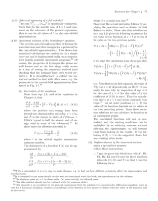
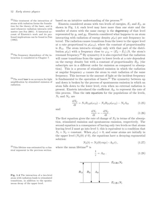
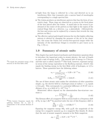
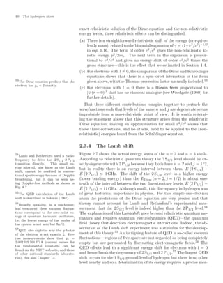
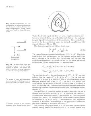
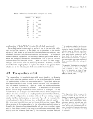
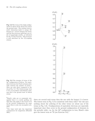
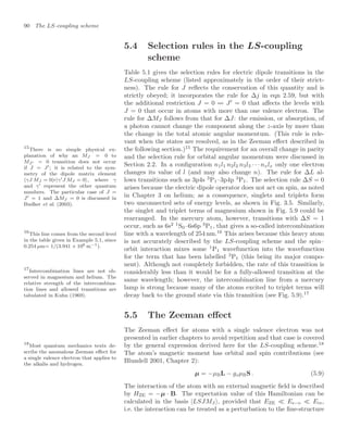
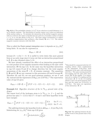
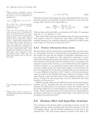
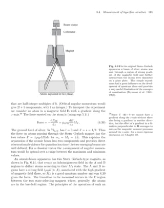
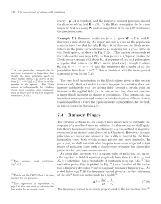
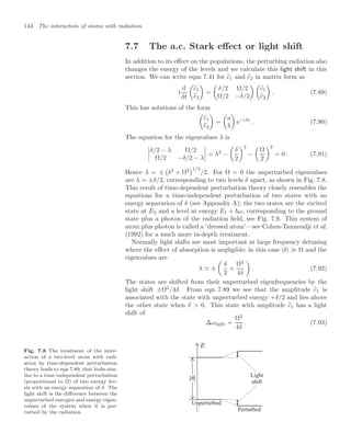
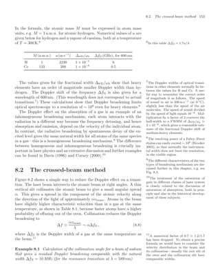
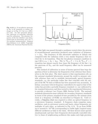
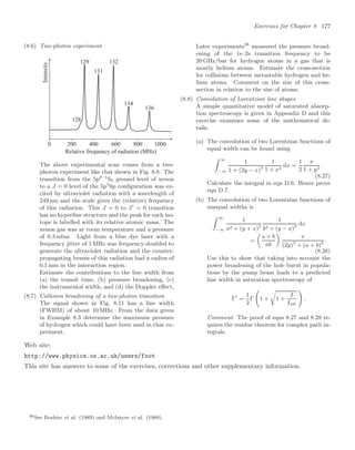
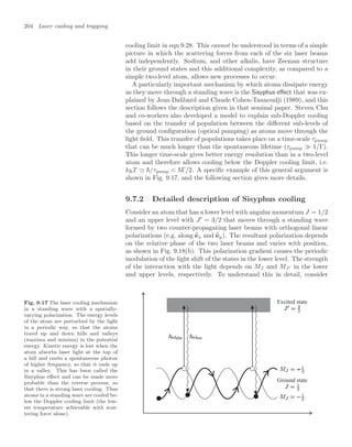
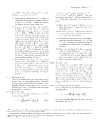
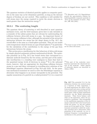
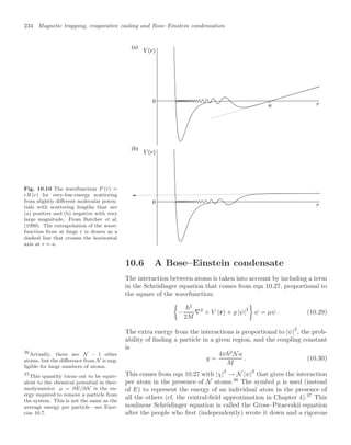
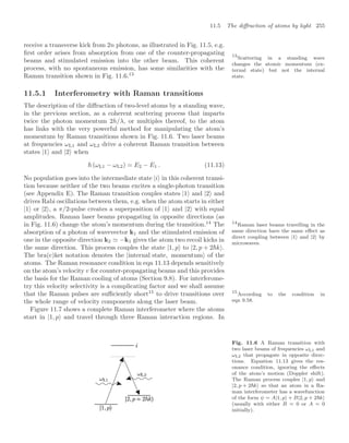
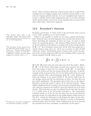
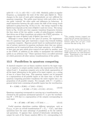
96. The LS-coupling scheme 81
Fig. 5.1 The residual electrostatic in-
teraction causes l1 and l2 to precess
around their resultant L = l1 + l2.
The interaction between the electrons, from their electrostatic repul-
sion, causes their orbital angular momenta to change, i.e. in the vector
model l1 and l2 change direction, but their magnitudes remain constant.
This internal interaction does not change the total orbital angular mo-
mentum L = l1 +l2, so l1 and l2 move (or precess) around this vector, as
illustrated in Fig. 5.1. When no external torque acts on the atom, L has
a fixed orientation in space so its z-component ML is also a constant of
the motion (ml1 and ml2 are not good quantum numbers). This classical
picture of conservation of total angular momentum corresponds to the
quantum mechanical result that the operators L2
and Lz both commute
with Hre:3
3
The proof is straightforward for the
quantum operator: Lz = l1z +l2z since
ml1
= q always occurs with ml2
= −q
in eqn 3.30.
!
L2
, Hre
= 0 and [Lz, Hre] = 0 . (5.2)
Since Hre does not depend on spin it must also be true that
!
S2
, Hre
= 0 and [Sz, Hre] = 0 . (5.3)
Actually, Hre also commutes with the individual spins s1 and s2 but
we chose eigenfunctions of S to antisymmetrise the wavefunctions, as
in helium—the spin eigenstates for two electrons are ψA
spin and ψS
spin for
S = 0 and 1, respectively.4
The quantum numbers L, ML, S and MS
4
The Hamiltonian H commutes with
the exchange (or swap) operator Xij
that interchanges the labels of the par-
ticles i ↔ j; thus states that are simul-
taneously eigenfunctions of both oper-
ators exist. This is obviously true for
the Hamiltonian of the helium atom in
eqn 3.1 (which looks the same if 1 ↔ 2),
but it also holds for eqn 5.1. In general,
swapping particles with the same mass
and charge does not change the Hamil-
tonian for the electrostatic interactions
of a system.
have well-defined values in this Russell–Saunders or LS-coupling scheme.
Thus the eigenstates of Hre are |LMLSMS . In the LS-coupling scheme
the energy levels labelled by L and S are called terms (and there is
degeneracy with respect to ML and MS). We saw examples of 1
L and
3
L terms for the 1snl configurations in helium where the LS-coupling
scheme is a very good approximation. A more complex example is an
npn
p configuration, e.g. 3p4p in silicon, that has six terms as follows:
l1 = 1, l2 = 1 ⇒ L = 0, 1 or 2 ,
s1 =
1
2
, s2 =
1
2
⇒ S = 0 or 1 ;
terms: 2S+1
L = 1
S, 1
P, 1
D, 3
S, 3
P, 3
D .
The direct and exchange integrals that determine the energies of these
terms are complicated to evaluate (see Woodgate (1980) for details)
and here we shall simply make some empirical observations based on
the terms diagrams in Figs 5.2 and 5.3. The (2l1 + 1) (2l2 + 1) = 9
degenerate states of orbital angular momentum become the 1 + 3 +
5 = 9 states of ML associated with the S, P and D terms, respectively.
As in helium, linear combinations of the four degenerate spin states
lead to triplet and one singlet terms but, unlike helium, triplets do not
necessarily lie below singlets. Also, the 3p2
configuration has fewer terms
than the 3p4p configuration for equivalent electrons, because of the Pauli
exclusion principle (see Exercise 5.6).
In the special case of ground configurations of equivalent electrons the
spin and orbital angular momentum of the lowest-energy term follow
some empirical rules, called Hund’s rules: the lowest-energy term has
the largest value of S consistent with the Pauli exclusion principle.5
If
5
Two electrons cannot both have the
same set of quantum numbers.

97. 82 The LS-coupling scheme
Fig. 5.2 The terms of the 3p4p configu-
ration in silicon all lie about 6 eV above
the ground state. The residual electro-
static interaction leads to energy dif-
ferences of ∼ 0.2 eV between the terms,
and the fine-structure splitting is an or-
der of magnitude smaller, as indicated
for the 3P and 3D terms. This structure
is well described by the LS-coupling
scheme.
6.4
6.3
6.2
6.1
6.0
5.8
5.9
Fig. 5.3 The energies of terms of the
3p2 configuration of silicon. For equiv-
alent electrons the Pauli exclusion prin-
ciple restricts the number of terms—
there are only three compared to the
six in Fig. 5.2. The lowest-energy term
is 3P, in accordance with Hund’s rules,
and this is the ground state of silicon
atoms.
2.0
0.0
0.2
0.4
0.6
0.8
1.2
1.4
1.6
1.8
1.0
there are several such terms then the one with the largest L is lowest.
The lowest term in Fig. 5.3 is consistent with these rules;6
the rule says
6
Hund’s rules are so commonly mis-
applied that it is worth spelling out
that they only apply to the lowest term
of the ground configuration for cases
where there is only one incomplete sub-
shell.
nothing about the ordering of the other terms (or about any of the
terms in Fig. 5.2). Configurations of equivalent electrons are especially
important since they occur in the ground configuration of elements in
the periodic table, e.g. for the 3d6
configuration in iron, Hund’s rules
give the lowest term as 5
D (see Exercise 5.6).7
7
The large total spin has important
consequences for magnetism (Blundell
2001).

98. 5.1 Fine structure in the LS-coupling scheme 83
5.1 Fine structure in the LS-coupling
scheme
Fine structure arises from the spin–orbit interaction for each of the un-
paired electrons given by the Hamiltonian
Hs−o = β1s1 · l1 + β2s2 · l2 .
For atoms with two valence electrons Hs−o acts as a perturbation on
the states |LMLSMS . In the vector model, this interaction between
the spin and orbital angular momentum causes L and S to change di-
rection, so that neither Lz nor Sz remains constant; but the total elec-
tronic angular momentum J = L + S, and its z-component Jz, are both
constant because no external torque acts on the atom. We shall now
evaluate the effect of the perturbation Hs−o on a term using the vec-
tor model. In the vector-model description of the LS-coupling scheme,
l1 and l2 precess around L, as shown in Fig. 5.4; the components per-
pendicular to this fixed direction average to zero (over time) so that
only the component of these vectors along L needs to be considered,
e.g. l1→
l1 · L
/ |L|2
L. The time average l1 · L in the vector model
becomes the expectation value l1 · L in quantum mechanics; also we
have to use L(L + 1) for the magnitude-squared of the vector. Applying
the same projection procedure to the spins leads to
Hs−o = β1
s1 · S
S (S + 1)
S ·
l1 · L
L (L + 1)
L + β2
s2 · S
S (S + 1)
S ·
l2 · L
L (L + 1)
L
= βLS S · L . (5.4)
Fig. 5.4 In the LS-coupling scheme
the orbital angular momenta of the two
electrons couple to give total angular
momentum L = l1 + l2. In the vec-
tor model l1 and l2 precess around L;
similarly, s1 and s2 precess around S.
L and S precess around the total an-
gular momentum J (but more slowly
than the precession of l1 and l2 around
L because the spin–orbit interaction is
‘weaker’ than the residual electrostatic
interaction).
The derivation of this equation by the vector model that argues by
analogy with classical vectors can be fully justified by reference to the
theory of angular momentum. It can be shown that, in the basis |J MJ
of the eigenstates of a general angular momentum operator J and its
component Jz, the matrix elements of any vector operator V are pro-
portional to those of J, i.e. J MJ| V |J MJ = c J MJ | J |J MJ .8
Fig-
8
This is particular case of a more
general result called the Wigner–
Eckart theorem which is the corner-
stone of the theory of angular momen-
tum. This powerful theorem also ap-
plies to off-diagonal elements such as
J MJ | V
J M
J
, and to more com-
plicated operators such as those for
quadrupole moments. It is used ex-
tensively in advanced atomic physics—
see the ‘Further reading’ section in this
chapter.
ure 5.5 gives a pictorial representation of why it is only the component of
V along J that is well defined. We want to apply this result to the case
where V = l1 or l2 in the basis of eigenstates |L ML , and analogously
for the spins. For L ML| l1 |L ML = c L ML| L |L ML the constant
c is determined by taking the dot product of both sides with L to give
c =
L ML| l1 · L |L ML
L ML| L · L |L ML
;
hence
L ML| l1 |L ML =
l1 · L
L(L + 1)
L ML| L |L ML . (5.5)
This is an example of the projection theorem and can also be applied to
l2 and to s1 and s2 in the basis of eigenstates |S MS . It is clear that,
for diagonal matrix elements, these quantum mechanical results give the
same result of the vector model.
Fig. 5.5 A pictorial representation of
the project theorem for an atom, where
J defines the axis of the system.

99. 84 The LS-coupling scheme
Equation 5.4 has the same form as the spin–orbit interaction for the
single-electron case but with capital letters rather than s·l. The constant
βLS that gives the spin–orbit interaction for each term is related to that
for the individual electrons (see Exercise 5.2). The energy shift is
Es−o = βLS S · L . (5.6)
To find this energy we need to evaluate the expectation value of the
operator L · S = (J · J − L · L − S · S) /2 for each term 2S+1
L. Each
term has (2S + 1) (2L + 1) degenerate states. Any linear combination
of these states is also an eigenstate with the same electrostatic energy
and we can use this freedom to choose suitable eigenstates and make the
calculation of the (magnetic) spin–orbit interaction straightforward. We
shall use the states |LSJMJ ; these are linear combinations of the basis
states |LMLSMS but we do not need to determine their exact form to
find the eigenenergies.9
Evaluation of eqn 5.6 with the states |LSJMJ
9
Similarly, in the one-electron case we
found the fine structure without deter-
mining the eigenstates |lsjmj explic-
itly in terms of the Yl,m and spin func-
tions.
gives
Es−o =
βLS
2
{ J (J + 1) − L (L + 1) − S (S + 1) } . (5.7)
Thus the energy interval between adjacent J levels is
∆EFS = EJ − EJ−1 = βLS J . (5.8)
This is called the interval rule. For example, a 3
P term (L = 1 = S) has
three J levels: 2S+1
LJ = 3
P0, 3
P1, 3
P2 (see Fig. 5.6); and the separation
between J = 2 and J = 1 is twice that between J = 1 and J = 0. The
existence of an interval rule in the fine structure of a two-electron system
generally indicates that the LS-coupling scheme is a good approximation
(see the ‘Exercises’ in this chapter); however, the converse is not true.
The LS-coupling scheme gives a very accurate description of the energy
levels of helium but the fine structure does not exhibit an interval rule
(see Example 5.2 later in this chapter).
Fig. 5.6 The fine structure of a 3P
term obeys the interval rule.
It is important not to confuse LS-coupling (or Russell–Saunders cou-
pling) with the interaction between L and S given by βLS S · L. In this
book the word interaction is used for real physical effects described by
a Hamiltonian and coupling refers to the forming of linear-combination
wavefunctions that are eigenstates of angular momentum operators, e.g.
eigenstates of L and S. The LS-coupling scheme breaks down as the
strength of the interaction βLS S · L increases relative to that of Hre.10
10
In classical mechanics the word ‘cou-
pling’ is commonly used more loosely,
e.g. for coupled pendulums, or coupled
oscillators, the ‘coupling between them’
is taken to mean the ‘interaction be-
tween them’ that leads to their motions
being coupled. (This coupling may take
the form of a physical linkage such as a
rod or spring between the two systems.)
5.2 The jj-coupling scheme
To calculate the fine structure in the LS-coupling scheme we treated the
spin–orbit interaction as a perturbation on a term, 2S+1
L. This is valid
when Ere Es−o, which is generally true in light atoms.11
The spin–
11
Es−o ∼ βLS and Ere is comparable
to the exchange integral. orbit interaction increases with atomic number (eqn 4.13) so that it can
be similar to Ere for heavy atoms—see Fig. 5.7. However, it is only in
cases with particularly small exchange integrals that Es−o exceeds Ere,
so that the spin–orbit interaction must be considered before the residual

100. 5.2 The jj-coupling scheme 85
Energy (eV)
1
Fine structure
Gross structure
Residual electrostatic energy
H
H
He
He
Na
Na
Mg
Mg
Cs
Cs
Hg
Hg
10 100
1
10
102
10−1
10−2
10−3
10−4
10−5
Fig. 5.7 A plot of typical energies as a
function of the atomic number Z (on
logarithmic scales). A characteristic
energy for the gross structure is taken
as the energy required to excite an elec-
tron from the ground state to the first
excited state—this is less than the ion-
ization energy but has a similar varia-
tion with Z. The residual electrostatic
interaction is the singlet–triplet separa-
tion of the lowest excited configuration
in some atoms with two valence elec-
trons. The fine structure is the split-
ting of the lowest p configuration. For
all cases the plotted energies are fairly
close to the maximum for that type
of structure in neutral atoms—higher-
lying configurations have smaller val-
ues.
electrostatic interaction. When Hs−o acts directly on a configuration it
causes the l and s of each individual electron to be coupled together to
give j1 = l1 + s1 and j2 = l2 + s2; in the vector model this corresponds
to l and s precessing around j independently of the other electrons.
In this jj-coupling scheme each valence electron acts on its own, as
in alkali atoms. For an sp configuration the s-electron can only have
j1 = 1/2 and the p-electron has j2 = 1/2 or 3/2; so there are two
levels, denoted by (j1, j2) = (1/2, 1/2) and (1/2, 3/2). The residual
electrostatic interaction acts as a perturbation on the jj-coupled levels;
it causes the angular momenta of the electrons to be coupled to give
total angular momentum J = j1 + j2 (as illustrated in Fig. 5.8). Since
there is no external torque on the atom, MJ is also a good quantum
number. For an sp configuration there are pairs of J levels for each of the
two original jj-coupled levels, e.g. (j1, j2)J = (1/2, 1/2)0 , (1/2, 1/2)1
and (1/2, 3/2)1 , (1/2, 3/2)2. This doublet structure, shown in Fig. 5.10,
contrasts with the singlets and triplets in the LS-coupling scheme.

101. 86 The LS-coupling scheme
Fig. 5.8 The jj-coupling scheme. The
spin–orbit interaction energy is large
compared to the Ere. (Cf. Fig. 5.4 for
the LS-coupling scheme.)
In summary, the conditions for LS- and jj-coupling are as follows:12
12
In both of these cases we assume an
isolated configuration, i.e. that the en-
ergy separation of the different config-
urations in the central field is greater
than the perturbation produced by ei-
ther Es−o or Ere.
LS-coupling scheme: Ere Es−o ,
jj-coupling scheme: Es−o Ere .
5.3 Intermediate coupling: the transition
between coupling schemes
In this section we shall look at examples of angular momentum coupling
schemes in two-electron systems. Figure 5.9 shows energy-level diagrams
of Mg and Hg and the following example looks at the structure of these
atoms.
Example 5.1
3s3p, Mg 6s6p, Hg
2.1850 3.76
2.1870 3.94
2.1911 4.40
3.5051 5.40
The table gives the energy levels, in units of 106
m−1
measured from
the ground state, for the 3s3p configuration in magnesium (Z = 12) and
6s6p in mercury (Z = 80). We shall use these data to identify the levels
and assign further quantum numbers.
For an sp configuration we expect 1
P and 3
P terms. In the case of
magnesium we see that the spacings between the three lowest levels are
2000 m−1
and 4100 m−1
; these are close to the 1 to 2 ratio expected from
the interval rule for the levels with J = 0, 1 and 2 that arise from the
triplet. The LS-coupling scheme gives an accurate description because

102. 5.3 Intermediate coupling: the transition between coupling schemes 87
−1
−2
−3
−4
−5
−6
−7
−8
−9
−10
−11
0
Hg
Mg
He
H Complex
terms
2
3
4
67
89
5
Fig. 5.9 The terms of helium, magnesium and mercury are plotted on the same energy scale (with hydrogen on the left for
comparison). The fine structure of the lighter atoms is too small to be seen on this scale and the LS-coupling scheme gives
a very accurate description. This scheme gives an approximate description for the low-lying terms of mercury even though it
has a much larger fine structure, e.g. for the 6s6p configuration the Ere Es−o but the interval rule is not obeyed because
the spin–orbit interaction is not very small compared to the residual electrostatic interaction. The 1s2 configuration of helium
is not shown; it has a binding energy of −24.6 eV (see Fig. 3.4). The 1s2s and 1s2p configurations of helium lie close to the
n = 2 shell in hydrogen, and similarly the 1s3l configurations lie close to the n = 3 shell. In magnesium, the terms of the
3snf configurations have very similar energies to those in hydrogen, but the differences get larger as l decreases. The energies
of the terms in mercury have large differences from the hydrogen energy levels. Much can be learnt by carefully studying this
term diagram, e.g. there is a 1P term which has similar energy in the three configurations: 1s2p, 3s3p and 6s6p in He, Mg and
Hg, respectively—thus the effective quantum number n∗ is similar despite the increase in n. Complex terms arise when both
valence electrons are excited in Mg, e.g. the 3p2 configuration, and the 5d96s26p configuration in Hg.

103. 88 The LS-coupling scheme
the fine structure is much smaller than the energy separation (Ere ∼
1.3 × 106
m−1
) between the 3
P term at ∼ 2.2 × 106
m−1
and the 1
P1
level at 3.5 × 106
m−1
. In mercury the spacings of the levels, going
down the table, are 0.18, 0.46 and 1.0 (in units of 106
m−1
); these
levels are not so clearly separated into a singlet and triplet. Taking the
lowest three levels as 3
P0, 3
P1 and 3
P2 we see that the interval rule is
not well obeyed since 0.46/0.18 = 2.6 (not 2).13
This deviation from
13
This identification of the levels is
supported by other information, e.g.
determination of J from the Zeeman ef-
fect and the theoretically predicted be-
haviour of an sp configuration shown in
Fig. 5.10.
the LS-coupling scheme is hardly surprising since this configuration has
a spin–orbit interaction only slightly smaller than the singlet–triplet
separation. However, even for this heavy atom, the LS-coupling scheme
gives a closer approximation than the jj-coupling scheme.
Fig. 5.10 A theoretical plot of the energy levels that arise from an sp configuration as a function of the strength of the
spin–orbit interaction parameter β (of the p-electron defined in eqn 2.55). For β = 0 the two terms, 3P and 1P, have an energy
separation equal to twice the exchange integral; this residual electrostatic energy is assumed to be constant and only β varies in
the plot. As β increases the fine structure of the triplet becomes observable. As β increases further the spin–orbit and residual
electrostatic interactions become comparable and the LS-coupling scheme ceases to be a good approximation: the interval rule
and (LS-coupling) selection rules break down (as in mercury, see Fig. 5.9). At large β the jj-coupling scheme is appropriate.
The operator J commutes with Hs−o (and Hre); therefore Hs−o only mixes levels of the same J, e.g. the two J = 1 levels in
this case. (The energies of the J = 0 and 2 levels are straight lines because their wavefunctions do not change.) Exercise 5.8
gives an example of this transition between the two coupling schemes for np(n + 1)s configurations with n = 3 to 5 (that have
small exchange integrals).

104. 5.3 Intermediate coupling: the transition between coupling schemes 89
Example 5.2 The 1s2p configuration in helium
J E (m−1
)
2 16 908 687
1 16 908 694
0 16 908 793
1 17 113 500
The table gives the values of J and the energy, in units of m−1
measured
from the ground state, for the levels of the 1s2p configuration in helium.
The 3
P term has a fine-structure splitting of about 100 m−1
that is
much smaller than the singlet–triplet separation of 106
m−1
from the
electrostatic interaction (twice the exchange integral). Thus the LS-
coupling scheme gives an excellent description of the helium atom and
the selection rules in Table 5.1 are well obeyed. But the interval rule is
not obeyed—the intervals between the J levels are 7 m−1
and 99 m−1
and
the fine structure is inverted. This occurs in helium because spin–spin
and spin–other-orbit interactions have an energy comparable with that of
the spin–orbit interaction.14
However, for atoms other than helium, the
14
The spin–spin interaction arises from
the interaction between two magnetic
dipoles (independent of any relative
motion). See eqn 6.12 and its expla-
nation.
rapid increase in the strength of the spin–orbit interaction with Z ensures
that Hs−o dominates over the others. Therefore the fine structure of
atoms in the LS-coupling scheme usually leads to an interval rule.
Further examples of energy levels are given in the exercises at the end
of this chapter. Figure 5.10 shows a theoretical plot of the transition
from the LS- to the jj-coupling scheme for an sp configuration. Conser-
vation of the total angular momentum means that J is a good quantum
number even in the intermediate coupling regime and can always be used
to label the levels. The notation 2S+1
LJ for the LS-coupling scheme is
often used even for systems in the intermediate regime and also for one-
electron systems, e.g. 1s 2
S1/2 for the ground state of hydrogen.
Table 5.1 Selection rules for electric dipole (E1) transitions in the LS-coupling
scheme. Rules 1–4 apply to all electric dipole transitions; rules 5 and 6 are obeyed
only when L and S are good quantum numbers. The right-hand column gives the
structure to which the rule applies.
1 ∆J = 0, ±1 (J = 0 J
= 0) Level
2 ∆MJ = 0, ±1 (MJ = 0 MJ = 0 if ∆J = 0) State
3 Parity changes Configuration
4 ∆l = ±1 One electron jump Configuration
5 ∆L = 0, ±1 (L = 0 L
= 0) Term
6 ∆S = 0 Term

105. 90 The LS-coupling scheme
5.4 Selection rules in the LS-coupling
scheme
Table 5.1 gives the selection rules for electric dipole transitions in the
LS-coupling scheme (listed approximately in the order of their strict-
ness). The rule for J reflects the conservation of this quantity and is
strictly obeyed; it incorporates the rule for ∆j in eqn 2.59, but with
the additional restriction J = 0 J
= 0 that affects the levels with
J = 0 that occur in atoms with more than one valence electron. The
rule for ∆MJ follows from that for ∆J: the emission, or absorption, of
a photon cannot change the component along the z-axis by more than
the change in the total atomic angular momentum. (This rule is rele-
vant when the states are resolved, as in the Zeeman effect described in
the following section.)15
The requirement for an overall change in parity
15
There is no simple physical ex-
planation of why an MJ = 0 to
MJ = 0 transition does not occur
if J = J; it is related to the sym-
metry of the dipole matrix element
γJ MJ = 0|r|γJ MJ = 0, where γ
and γ represent the other quantum
numbers. The particular case of J =
J = 1 and ∆MJ = 0 is discussed in
Budker et al. (2003).
and the selection rule for orbital angular momentum were discussed in
Section 2.2. In a configuration n1l1 n2l2 n3l3 · · · nxlx only one electron
changes its value of l (and may also change n). The rule for ∆L al-
lows transitions such as 3p4s 3
P1–3p4p 3
P1. The selection rule ∆S = 0
arises because the electric dipole operator does not act on spin, as noted
in Chapter 3 on helium; as a consequence, singlets and triplets form
two unconnected sets of energy levels, as shown in Fig. 3.5. Similarly,
the singlet and triplet terms of magnesium shown in Fig. 5.9 could be
rearranged. In the mercury atom, however, transitions with ∆S = 1
occur, such as 6s2 1
S0–6s6p 3
P1, that gives a so-called intercombination
line with a wavelength of 254 nm.16
This arises because this heavy atom
16
This line comes from the second level
in the table given in Example 5.1, since
0.254 µm= 1/(3.941 × 106 m−1).
is not accurately described by the LS-coupling scheme and the spin–
orbit interaction mixes some 1
P1 wavefunction into the wavefunction
for the term that has been labelled 3
P1 (this being its major compo-
nent). Although not completely forbidden, the rate of this transition is
considerably less than it would be for a fully-allowed transition at the
same wavelength; however, the intercombination line from a mercury
lamp is strong because many of the atoms excited to triplet terms will
decay back to the ground state via this transition (see Fig. 5.9).17
17
Intercombination lines are not ob-
served in magnesium and helium. The
relative strength of the intercombina-
tion lines and allowed transitions are
tabulated in Kuhn (1969).
5.5 The Zeeman effect
The Zeeman effect for atoms with a single valence electron was not
presented in earlier chapters to avoid repetition and that case is covered
by the general expression derived here for the LS-coupling scheme.18
18
Most quantum mechanics texts de-
scribe the anomalous Zeeman effect for
a single valence electron that applies to
the alkalis and hydrogen.
The atom’s magnetic moment has orbital and spin contributions (see
Blundell 2001, Chapter 2):
µ = −µBL − gsµBS . (5.9)
The interaction of the atom with an external magnetic field is described
by HZE = −µ · B. The expectation value of this Hamiltonian can be
calculated in the basis |LSJMJ , provided that EZE Es−o Ere,
i.e. the interaction can be treated as a perturbation to the fine-structure

106. 5.5 The Zeeman effect 91
levels of the terms in the LS-coupling scheme. In the vector model we
project the magnetic moment onto J (see Fig. 5.11) following the same
rules as are used in treating fine structure in the LS-coupling scheme
(and taking B = B
ez). This gives
Fig. 5.11 The projection of the
contributions to the total magnetic
moment from the orbital motion and
the spin are projected along J.
HZE = −
µ · J
J (J + 1)
J · B =
L · J + gs S · J
J (J + 1)
µBBJz . (5.10)
In the vector model the quantities in angled brackets are time averages.19
19
Components perpendicular to J
time-average to zero.
In a quantum description treatment the quantities · · · are expectation
values of the form J MJ | · · · |J MJ .20
In the vector model
20
This statement is justified by the pro-
jection theorem (Section 5.1), derived
from the more general Wigner–Eckart
theorem. The theorem shows that the
expectation value of the vector opera-
tor L is proportional to that of J in the
basis of eigenstates |J MJ , i.e.
J MJ | L |J MJ ∝ J MJ | J |J MJ ,
and similarly for the expectation value
of S. The component along the mag-
netic field is found by taking the dot
product with B:
J MJ | L · B |J MJ
∝ J MJ | J · B |J MJ
∝ J MJ | Jz |J MJ = MJ .
EZE = gJ µBBMJ , (5.11)
where the Landé g-factor is gJ = { L · J + gs S · J } / {J (J + 1)} . As-
suming that gs 2 (see Section 2.3.4) gives
gJ =
3
2
+
S (S + 1) − L (L + 1)
2J (J + 1)
. (5.12)
Singlet terms have S = 0 so J = L and gJ = 1 (no projection is nec-
essary). Thus singlets all have the same Zeeman splitting between MJ
states and transitions between singlet terms exhibit the normal Zeeman
effect (shown in Fig. 5.12). The ∆MJ = ±1 transitions have frequencies
shifted by ±µBB/h with respect to the ∆MJ = 0 transitions.
In atoms with two valence electrons the transitions between triplet
terms exhibit the anomalous Zeeman effect. The observed pattern de-
pends on the values of gJ and J for the upper and lower levels, as shown
in Fig. 5.13. In both the normal and anomalous effects the π-transitions
(∆MJ = 0) and σ-transitions (∆MJ = ±1) have the same polarizations
as in the classical model in Section 1.8. Other examples in Exercises 5.10
to 5.12 show how observation of the Zeeman pattern gives information
about the angular momentum coupling in the atom. (The Zeeman ef-
fect observed for the 2
P1/2–2
S1/2 and 2
P3/2–2
S1/2 transitions that arise
between the fine-structure components of the alkalis and hydrogen is
treated in Exercise 5.13.) Exercise 5.14 goes through the Paschen–Back
effect that occurs in a strong external magnetic field—see Fig. 5.14.

107. 92 The LS-coupling scheme
Fig. 5.12 The normal Zeeman effect
on the 1s2p 1P1–1s3d 1D2 line in he-
lium. These levels split into three and
five MJ states, respectively. Both lev-
els have S = 0 and gJ = 1 so that the
allowed transitions between the states
give the same pattern of three compo-
nents as the classical model (in Sec-
tion 1.8)—this is the historical reason
why it is called the normal Zeeman ef-
fect. Spectroscopists called any other
pattern an anomalous Zeeman effect,
although such patterns have a straight-
forward explanation in quantum me-
chanics and arise whenever S = 0,
e.g. all atoms with one valence elec-
tron have S = 1/2. The π- and σ-
components arise from ∆MJ = 0 and
∆MJ = ±1 transitions, respectively.
(In this example of the normal Zeeman
effect each component corresponds to
three allowed electric dipole transitions
with the same frequency but they are
drawn with a slight horizontal separa-
tion for clarity.)
2
1
0
−1
−2
1
0
−1
Frequency
Fig. 5.13 The anomalous Zeeman ef-
fect for the 6s6p 3P2–6s7s 3S1 transi-
tion in Hg. The lower and upper levels
both have the same number of Zeeman
sub-levels (or MJ states) as the levels in
Fig. 5.12, but give rise to nine separate
components because the levels have dif-
ferent values of gJ . (The 6s7s config-
uration happens to have higher energy
than 6s6p, as shown in Fig. 5.9, but the
Zeeman pattern does not depend on the
relative energy of the levels.)
1
1
2
0
−1
−2
0
−1
Frequency

108. 5.6 Summary 93
B
S
L
Fig. 5.14 The Paschen–Back effect oc-
curs in a strong external magnetic field.
The spin and orbital angular momen-
tum precess independently about the
magnetic field. The states have ener-
gies given by EPB = µBB(ML + 2MS).
5.6 Summary
Figure 5.15 shows the different layers of structure in a case where the
LS-coupling scheme is a good approximation, i.e. the residual electro-
static interaction dominates the two magnetic interactions (spin–orbit
and with an external magnetic field). The spin–orbit interaction splits
terms into different J levels. The Zeeman effect of a weak magnetic
field splits the levels into states of given MJ , that are also referred to as
Zeeman sub-levels.
There are various ways in which this simple picture can break down.
(a) Configuration mixing occurs if the residual electrostatic interaction
Configuration Levels States
Terms
1
2
0
−1
−2
0
−1
1
0
0
−1
1
Fig. 5.15 The hierarchy of atomic structure for the 3s3p configuration of an alkaline earth metal atom.

109. 94 The LS-coupling scheme
is not small compared to the energy gap between the configurat-
ions—this is common in atoms with complex electronic structure.
(b) The jj-coupling scheme is a better approximation than LS-coupling
or Russell–Saunders coupling when the spin–orbit interaction is
greater than the residual electrostatic interaction.
(c) The Paschen–Back effect arises when the interaction with an exter-
nal magnetic field is stronger than the spin–orbit interaction (with
the internal field). This condition is difficult to achieve except for
atoms with a low atomic number and hence small fine structure.
Similar physics arises in the study of the Zeeman effect on hyperfine
structure where the transition between the low-field and high-field
regimes occurs at values of the magnetic field that are easily acces-
sible in experiments (see Section 6.3).
Further reading
The mathematical methods that describe the way in which angular
momenta couple together form the backbone of the theory of atomic
structure. In this chapter the quantum mechanical operators have been
treated by analogy with classical vectors (the vector model) and the
Wigner–Eckart theorem was mentioned to justify the projection theo-
rem. Graduate-level texts give a more comprehensive discussion of the
quantum theory of angular momentum, e.g. Cowan (1981), Brink and
Satchler (1993) and Sobelman (1996).
Exercises
(5.1) Description of the LS-coupling scheme
Explain what is meant by the central-field approx-
imation and show how it leads to the concept of
electron configurations. Explain how perturba-
tions arising from (a) the residual electrostatic in-
teractions, and (b) the magnetic spin–orbit inter-
actions, modify the structure of an isolated multi-
electron configuration in the LS-coupling limit.
(5.2) Fine structure in the LS-coupling scheme
Show from eqn 5.4 that the J levels of the 3
P term
in the 3s4p configuration have a separation given
by eqn 5.8 with βLS = β4p/2 (where β4ps · l is the
spin–orbit interaction of the 4p-electron).
(5.3) The LS-coupling scheme and the interval rule in
calcium
Write down the ground configuration of calcium
(Z = 20). The line at 610 nm in the spectrum
of neutral calcium consists of three components
at relative positions 0, 106 and 158 (in units of
cm−1
). Identify the terms and levels involved in
these transitions.
The spectrum also contains a multiplet of six lines
with wavenumbers 5019, 5033, 5055, 5125, 5139
and 5177 (in units of cm−1
). Identify the terms
and levels involved. Draw a diagram of the rel-
evant energy levels and the transitions between
them. What further experiment could be carried
out to check the assignment of quantum numbers?
(5.4) The LS-coupling scheme in zinc
The ground configuration of zinc is 4s2
. The
seven lowest energy levels of zinc are 0, 32 311,
32 501, 32 890, 46 745, 53 672 and 55 789 (in units
of cm−1
). Sketch an energy-level diagram that
shows these levels with appropriate quantum num-
bers. What evidence do these levels provide that

110. Exercises for Chapter 5 95
the LS-coupling scheme describes this atom. Show
the electric dipole transitions that are allowed be-
tween the levels.
(5.5) The LS-coupling scheme
3s3p, Mg 3s3p, Fe14+
2.1850 23.386
2.1870 23.966
2.1911 25.378
3.5051 35.193
The table gives the energy levels, in units of
106
m−1
measured from the ground state, of the
3s3p configuration in neutral magnesium (Z =
12) and the magnesium-like ion Fe14+
. Suggest,
with reasons, further quantum numbers to iden-
tify these levels. Calculate the ratio of the spin–
orbit interaction energies in the 3s3p configura-
tion of Mg and Fe14+
, and explain your result.
Discuss the occurrence in the solar spectrum of
a strong line at 41.726 nm that originates from
Fe14+
. Would you expect a corresponding tran-
sition in neutral Mg?
(5.6) LS-coupling for configurations with equivalent
electrons
(a) List the values of the magnetic quantum num-
bers ml1 , ms1 , ml2 and ms2 for the two elec-
trons in an np2
configuration to show that fif-
teen degenerate states exist within the central-
field approximation. Write down the values of
ML = ml1 +ml2 and MS = ms1 +ms2 associ-
ated with each of these states to show that the
only possible terms in the LS-coupling scheme
are 1
S, 3
P and 1
D.
(b) The 1s2
2s2
2p2
configuration of doubly-ionized
oxygen has levels at relative positions 0, 113,
307, 20 271 and 43 184 (in units of cm−1
)
above the ground state, and its spectrum con-
tains weak emission lines at 19 964 cm−1
and
20 158 cm−1
. Identify the quantum numbers
for each of the levels and discuss the extent to
which the LS-coupling scheme describes this
multiplet.
(c) For six d-electrons, in the same sub-shell,
write a list of the values of the ms and ml
for the individual electrons corresponding to
MS = 2 and ML = 2. Briefly discuss why this
is the maximum value of MS, and why ML ⩽ 2
for this particular value of MS. (Hence from
Hund’s rules the 5
D term has the lowest en-
ergy.) Specify the lowest-energy term for each
of the five configurations nd, nd2
, nd3
, nd4
and nd5
.
(5.7) Transition from LS- to jj-coupling
3p4s, Si
J Energy (106
m−1
)
0 3.968
1 3.976
2 3.996
1 4.099
3p7s, Si
J Energy (106
m−1
)
0 6.154
1 6.160
2 6.182
1 6.188
The table gives J-values and energies (in units of
106
m−1
measured from the ground state) of the
levels in the 3p4s and 3p7s configurations of sili-
con. Suggest further quantum numbers to identify
the levels.
Why do the two configurations have nearly the
same value of EJ=2 − EJ=0 but quite different en-
ergy separations between the two J = 1 states?
(5.8) Angular-momentum coupling schemes
4p5s, germanium
J Energy (106
m−1
)
0 3.75
1 3.77
2 3.91
1 4.00
5p6s, tin
J Energy (106
m−1
)
0 3.47
1 3.49
2 3.86
1 3.93
The table gives the J-values and energies (in units
of 106
m−1
measured from the ground state) of the
levels in the configurations 4p5s in Ge and 5p6s in
Sn. Data for the 3p4s configuration in Si are given
in the previous exercise. How well does the LS-
coupling scheme describe the energy levels of the
np(n + 1)s configurations with n = 3, 4 and 5?
Give a physical reason for the observed trends in
the energy levels.
One of the J = 1 levels in Ge has a Landé g-factor
of gJ = 1.06. Which level would you expect this
to be and why?
(5.9) Selection rules in the LS-coupling scheme
State the selection rules that determine the config-
urations, terms and levels that can be connected
by an electric dipole transition in the LS-coupling
approximation. Explain which rules are rigorous,
and which depend on the validity of the coupling

111. 96 The LS-coupling scheme
scheme. Give a physical justification for three of
these rules.
Which of the following are allowed for electric
dipole transitions in the LS-coupling scheme:
(a) 1s2s 3
S1–1s3d 3
D1,
(b) 1s2p 3
P1–1s3d 3
D3,
(c) 2s2p 3
P1–2p2 3
P1,
(d) 3p2 3
P1–3p2 3
P2,
(e) 3p6 1
S0–3p5
3d 1
D2?
The transition 4d9
5s2 2
D5/2–4d10
5p 2
P3/2 satis-
fies the selection rules for L, S and J but it ap-
pears to involve two electrons jumping at the same
time. This arises from configuration mixing—the
residual electrostatic interaction may mix configu-
rations.21
The commutation relations in eqns 5.2
and 5.3 imply that Hre only mixes terms of the
same L, S and J. Suggest a suitable configuration
that gives rise to a 2
P3/2 level that could mix with
the 4d10
5p configuration to cause this transition.
(5.10) The anomalous Zeeman effect
What selection rule governs ∆MJ in electric dipole
transitions? Verify that the 3
S1–3
P2 transition
leads to the pattern of nine equally-spaced lines
shown in Fig. 5.13 when viewed perpendicular to
a weak magnetic field. Find the spacing for a mag-
netic flux density of 1 T.
(5.11) The anomalous Zeeman effect
Draw an energy-level diagram for the states of 3
S1
and 3
P1 levels in a weak magnetic field. Indi-
cate the allowed electric dipole transitions between
the Zeeman states. Draw the pattern of lines ob-
served perpendicular to the field on a frequency
scale (marked in units of µBB/h).
(5.12) The anomalous Zeeman effect
Frequency
2 2 3 2 2 3 2 2
The above Zeeman pattern is observed for a spec-
tral line that originates from one of the levels of a
3
P term in the spectrum of a two-electron system;
the numbers indicate the relative separations of
the lines, observed perpendicular to the direction
of the applied magnetic field. Identify L, S and J
for the two levels in the transition.22
(5.13) The anomalous Zeeman effect in alkalis
Note that atoms with one valence electron are not
discussed explicitly in the text.
(a) Give the value of gJ for the one-electron levels
2
S1/2, 2
P1/2 and 2
P3/2.
(b) Show that the Zeeman pattern for the
3s 2
S1/2–3p 2
P3/2 transition in sodium has
six equally-spaced lines when viewed perpen-
dicular to a weak magnetic field. Find the
spacing (in GHz) for a magnetic flux density
of 1 T. Sketch the Zeeman pattern observed
along the magnetic field.
(c) Sketch the Zeeman pattern observed per-
pendicular to a weak magnetic field for the
3s 2
S1/2–3p 2
P1/2 transition in sodium.
(d) The two fine-structure components of the 3s–
3p transition in sodium in parts (b) and (c)
have wavelengths of 589.6 nm and 589.0 nm,
respectively. What magnetic flux density pro-
duces a Zeeman splitting comparable with the
fine structure?23
(5.14) The Paschen–Back effect
In a strong magnetic field L and S precess in-
dependently about the field direction (as shown
in Fig. 5.14), so that J and MJ are not good
quantum numbers and appropriate eigenstates are
|LMLSMS. This is called the Paschen–Back ef-
fect. In this regime the LS-coupling selection rules
are ∆ML = 0, ±1 and ∆MS = 0 (because the elec-
tric dipole operator does not act on the spin).24
Show that the Paschen–Back effect leads to a pat-
tern of three lines with the same spacing as in the
normal Zeeman effect (i.e. the same as if we com-
pletely ignore spin).25
21In the discussion of the LS-coupling scheme we treated Hre as a perturbation on a configuration and assumed that Ere
is small compared to the energy separation between the configurations in the central field. This is rarely true for high-lying
configurations of complex atoms.
22The relative intensities of the components have not been indicated.
23This value is greater than 1 T so the assumption of a weak field in part (b) is valid.
24The rules for J and MJ are not relevant in this regime.
25The Paschen–Back effect occurs when the valence electrons interact more strongly with the external magnetic field than
with the orbital field in Hs−o. The LS-coupling scheme still describes this system, i.e. L and S are good quantum numbers.

112. Hyperfine structure and
isotope shift
6
6.1 Hyperfine structure 97
6.2 Isotope shift 105
6.3 Zeeman effect and
hyperfine structure 108
6.4 Measurement of
hyperfine structure 112
Further reading 119
Exercises 120
6.1 Hyperfine structure
Up to this point we have regarded the nucleus as an object of charge
+Ze and mass MN, but it has a magnetic moment µI that is related to
the nuclear spin I by
µI = gI µN I . (6.1)
Comparing this to the electron’s magnetic moment −gs µB s we see that
there is no minus sign.1
Nuclei have much smaller magnetic moments
1
Nuclear magnetic moments can be
parallel, or anti-parallel, to I, i.e. gI
can have either sign depending on the
way that the spin and orbital angular
momenta of the protons and neutrons
couple together inside the nucleus. The
proton (that forms the nucleus of a hy-
drogen atom) has gp 0 because of
its positive charge. More generally, nu-
clear magnetic moments can be pre-
dicted from the shell model of the nu-
cleus.
than electrons; the nuclear magneton µN is related to the Bohr magneton
µB by the electron-to-proton mass ratio:
µN = µB
me
Mp
µB
1836
. (6.2)
The interaction of µI with the magnetic flux density created by the
atomic electrons Be gives the Hamiltonian
HHFS = −µI · Be . (6.3)
This gives rise to hyperfine structure which, as its name suggests, is
smaller than fine structure. Nevertheless, it is readily observable for
isotopes that have a nuclear spin (I = 0).
The magnetic field at the nucleus is largest for s-electrons and we
shall calculate this case first. For completeness the hyperfine structure
for electrons with l = 0 is also briefly discussed, as well as other effects
that can have similar magnitude.
6.1.1 Hyperfine structure for s-electrons
We have previously considered the atomic electrons as having a charge
distribution of density −e |ψ (r)|
2
, e.g. in the interpretation of the direct
integral in helium in eqn 3.15 (see also eqn 6.22). To calculate mag-
netic interactions we need to consider an s-electron as a distribution of
magnetisation given by
M = −gsµBs |ψ (r)|
2
. (6.4)
This corresponds to the total magnetic moment of the electron −gsµBs
spread out so that each volume element d3
r has a fraction |ψ (r)|2
d3
r

113. 98 Hyperfine structure and isotope shift
Fig. 6.1 (a) An illustration of a nu-
cleus with spin I surrounded by the
spherically-symmetric probability dis-
tribution of an s-electron. (b) That
part of the s-electron distribution in the
region r rb corresponds to a sphere
of magnetisation M anti-parallel to the
spin s.
(b)
(a)
of the total. For s-electrons this distribution is spherically symmetric
and surrounds the nucleus, as illustrated in Fig. 6.1. To calculate the
field at r = 0 we shall use the result from classical electromagnetism2
2
See Blundell (2001) or electromag-
netism texts. that inside a uniformly magnetised sphere the magnetic flux density is
Be =
2
3
µ0 M . (6.5)
However, we must be careful when applying this result since the distri-
bution in eqn 6.4 is not uniform—it is a function of r. We consider the
spherical distribution in two parts.
(a) A sphere of radius r = rb, where rb a0 so that the electronic
wavefunction squared has a constant value of |ψ (0)|2
throughout
this inner region, as indicated on Fig. 6.2.3
From eqn 6.5 the field
3
This spherical boundary at r = rb
does not correspond to anything physi-
cal in the atom but is chosen for math-
ematical convenience. The radius rb
should be greater than the radius of the
nucleus rN and it easy to fulfil the con-
ditions rN rb a0 since typical nu-
clei have a size of a few fermi (10−15 m),
which is five orders of magnitude less
than atomic radii.
inside this uniformly magnetised sphere is
Be = −
2
3
µ0 gsµB |ψns (0)|
2
s . (6.6)
(b) The part of the distribution outside the sphere r rb produces no
field at r = 0, as shown by the following argument. Equation 6.5
for the field inside a sphere does not depend on the radius of that
sphere—it gives the same field for a sphere of radius r and a sphere of
radius r+dr. Therefore the contribution from each shell of thickness
dr is zero. The region r rb can be considered as being made up of
many such shells that give no additional contribution to the field.4
4
The magnetisation is a function of
r only and therefore each shell has a
uniform magnetisation M(r) between r
and r + dr. The proof that these shells
do not produce a magnetic flux den-
sity at r = 0 does not require M (r)
to be the same for all the shells, and
clearly this is not the case. Alterna-
tively, this result can be obtained by in-
tegrating the contributions to the field
at the origin from the magnetic mo-
ments M(r) d3r over all angles (θ and
φ).
Putting this field and µI from eqn 6.1 into eqn 6.3 gives
HHFS = gIµN I ·
2
3
µ0 gsµB |ψns (0)|
2
s = A I · s . (6.7)

114. 6.1 Hyperfine structure 99
Fig. 6.2 (a) The probability density |ψ (r)|2
of an s-electron at small distances (r
a0) is almost constant. The distribution of nuclear matter ρN(r) gives an indication
of the nuclear radius rN. To calculate the interaction of the nuclear magnetic moment
with an s-electron the region is divided into two parts by a boundary surface of radius
r = rb rN (as also shown in Fig. 6.1). The inner region corresponds to a sphere
of uniform magnetisation that produces a flux density Be at r = 0. The nuclear
magnetic moment interacts with this field.
This is called the Fermi contact interaction since it depends on |ψns (0)|
2
being finite. It can also be expressed as
HHFS = A I · J (6.8)
because J = s for l = 0. It is useful to write down this more general
form at an early stage since it turns out that an interaction proportional
to I · J is also obtained when l = 0.
We have already considered the effect of an interaction proportional
to a dot product of two angular momenta when looking at the spin–orbit
interaction β S · L (eqn 5.4). In the same way the hyperfine interaction
in eqn 6.8 causes I and J to change direction but the total angular
momentum of the atom F = I + J remains constant. The quantities
I · B and J · B are not constant in this precession of I and J around F.
Therefore MI and MJ are not good quantum numbers; we use F and
MF instead and the eigenstates of HHFS are |IJFMF .5
The expectation
5
This should be compared with the LS-
coupling scheme where combinations
of the eigenstates |LMLSMS form
eigenstates of the spin–orbit interaction
|LSJMJ . The same warning issued for
LS-coupling and the spin–orbit inter-
action βS · L also applies. It is impor-
tant not to confuse IJ-coupling and the
interaction AI · J. In the IJ-coupling
scheme I and J are good quantum num-
bers and the states are |IJMI MJ or
|IJF MF . The latter are eigenstates
of the interaction AI · J.
value of eqn 6.8 gives
EHFS = A I · J =
A
2
{F(F + 1) − I(I + 1) − J(J + 1)} . (6.9)
Example 6.1 Hyperfine structure of the 1s 2
S1/2 ground state of hy-
drogen
The lowest level of the hydrogen atom is 1s 2
S1/2, i.e. J = 1
2 and the
proton has spin I = 1/2 so that F = 0 and 1 and these hyperfine levels
have energies
EHFS =
A
2
{F(F + 1) − I(I + 1) − J(J + 1)} =
A/4 for F = 1 ,
−3A/4 for F = 0 .
Fig. 6.3 The splitting between the hy-
perfine levels in the ground state of hy-
drogen.
The splitting between the hyperfine levels is ∆EHFS = A (see Fig. 6.3).
Substituting for |ψns (0)|
2
from eqn 2.22 gives
A =
2
3
µ0 gsµB gIµN
Z3
π a3
0 n3
. (6.10)

115. 100 Hyperfine structure and isotope shift
The proton has a g-factor of gI = 5.6, so for n = 1 = Z we have
∆EHFS
h
= 1.42 GHz .
This is very close to the measured value of 1 420 405 751.7667±0.0009Hz.
This frequency has been measured to such extremely high precision be-
cause it forms the basis of the hydrogen maser, described below.6
6
This hyperfine transition in hydrogen
is the one detected in radio astronomy,
where it is commonly referred to by its
wavelength as the 21 cm line.
6.1.2 Hydrogen maser
Maser stands for microwave amplification by stimulated emission of radi-
ation and such devices were the precursors of lasers, although nowadays
they are less widespread than the devices using light. Actually, lasers are
usually operated as oscillators rather than amplifiers but the acronym
with ‘o’ instead of ‘a’ is not so good. A schematic of a hydrogen maser
is shown in Fig. 6.4; it operates in the following way.
• Molecular hydrogen is dissociated in an electrical discharge.
• Atoms effuse from the source to form a beam in an evacuated chamber.
• The atoms pass through a region with a strong magnetic field gradient
(from a hexapole magnet) that focuses atoms in the upper hyperfine
level (F = 1) into a glass bulb. The atomic beam contains atoms in
both hyperfine levels but the state selection by the magnet7
leads to a
7
This works on the same basic princi-
ple as the Stern–Gerlach experiment in
Section 6.4.
Fig. 6.4 The hydrogen maser. The
principle of operation is described in
the text. A magnetic shield excludes
external fields and the solenoid cre-
ates a small stable magnetic field. In
this way the frequency shift produced
by the Zeeman effect on the hyperfine
structure is controlled (in the same way
as in the atomic clock described in Sec-
tion 6.4.2).
H source
State
selector
Magnetic
shield
Microwave
cavity
Microwave
output
Solenoid
Storage
bulb
Atoms in states
and

116. 6.1 Hyperfine structure 101
population inversion in the bulb, i.e. the population in F = 1 exceeds
that in F = 0; this gives more stimulated emission than absorption
and hence gain, or amplification of radiation at the frequency of the
transition.
• The atoms bounce around inside the bulb—the walls have a ‘non-stick’
coating of teflon so that collisions do not change the hyperfine level.
• The surrounding microwave cavity is tuned to the 1.42 GHz hyperfine
frequency and maser action occurs when there are a sufficient number
of atoms in the upper level. Power builds up in a microwave cavity,
some of which is coupled out through a hole in the wall of the cavity.
The maser frequency is very stable—much better than any quartz
crystal used in watches. However, the output frequency is not precisely
equal to the hyperfine frequency of the hydrogen atoms because of the
collisions with the walls (see Section 6.4).
6.1.3 Hyperfine structure for l = 0
Electrons with l = 0, orbiting around the nucleus, give a magnetic field
Be =
µ0
4π
−ev × (−r)
r3
−
µe − 3 (µe ·
r)
r
r3
, (6.11)
where −r gives the position of the nucleus with respect to the orbiting
electron. The first term arises from the orbital motion.8
It contains
8
This resembles the Biot–Savart law of
electromagnetism:
B =
µ0
4π
I ds × r
r3
.
Roughly speaking, the displacement
along the direction of the current is re-
lated to the electron’s velocity by ds =
v dt, where dt is a small increment of
time, and the current is related to the
charge by I dt = Q.
The spin–orbit interaction can be very
crudely ‘justified’ in a similar way, by
saying that the electron ‘sees’ the nu-
cleus of charge +Ze moving round it;
for a hydrogenic system this simplistic
argument gives
Borbital = −2Z
µ0
4π
µB
r3
l .
The Thomas precession factor does not
occur in hyperfine structure because
the frame of reference is not rotating.
the cross-product of −ev with −r, the position vector of the nucleus
relative to the electron, and −er × v = −2µBl. The second term is just
the magnetic field produced by the spin dipole moment of the electron
µe = −2µBs (taking gs = 2) at a position −r with respect to the dipole.9
9
See Blundell (2001).
Thus we can write
Be = −2
µ0
4π
µB
r3
l − s +
3 (s · r) r
r2
. (6.12)
This combination of orbital and spin–dipolar fields has a complicated
vector form.10
However, we can again use the argument (in Section 5.1)
10
The same two contributions to the
field also occur in the fine structure of
helium; the field produced at the po-
sition of one electron by the orbital
motion of the other electron is called
the spin–other-orbit interaction, and a
spin–spin interaction arises from the
field produced by the magnetic dipole
of one electron at the other electron.
that in the vector model there is rapid precession around J, and any
components perpendicular to this quantisation axis average to zero, so
that only components along J have a non-zero time-averaged value.11
11
In quantum mechanics this corre-
sponds to saying that the matrix
elements of any vector operator in
the eigenbasis |J MJ are propor-
tional to J, i.e. J MJ | Be |J MJ ∝
J MJ | J |J MJ . This is a consequence
of the Wigner–Eckart theorem that was
mentioned in Section 5.1.
The projection factor can be evaluated exactly (Woodgate 1980) but we
shall assume that it is approximately unity giving
Be ∼ −2
µ0
4π
.µB
r3
/
J . (6.13)
Thus from eqns 6.1 and 6.3 we find that the hyperfine interaction for
electrons with l = 0 has the same form AI · J as eqn 6.8. This form of
interaction leads to the following interval rule for hyperfine structure:
EF − EF −1 = A F . (6.14)
This interval rule is derived in the same way as eqn 5.8 for fine structure
but with I, J and F instead of L, S and J, as shown in Exercise 6.5.

117. 102 Hyperfine structure and isotope shift
Table 6.1 Comparison of fine and hyperfine structures.
Fine structure in the Hyperfine structure in the
LS-coupling scheme IJ-coupling scheme
Interaction β L · S A I · J
Total angular momentum J = L + S F = I + J
Eigenstates |LSJMJ |IJFMF
Energy, E β
2
{J (J + 1) − L (L + 1) − S (S + 1)} A
2
{F (F + 1) − I (I + 1) − J (J + 1)}
EJ − EJ−1 = βJ EF − EF −1 = AF
Interval rule
(if Es−o Ere) (if A ∆EQuadrupole)
That exercise also shows how this rule can be used to deduce F and
hence the nuclear spin I from a given hyperfine structure.12
12
This interval rule for magnetic dipole
hyperfine structure can be disrupted by
the quadrupole interaction. Some nu-
clei are not spherical and their charge
distribution has a quadrupole moment
that interacts with the gradient of the
electric field at the nucleus. This elec-
tric quadrupole interaction turns out to
have an energy comparable to the inter-
action of the magnetic dipole moment
µI with Be. Nuclei, and atoms, do not
have static electric dipole moments (for
states of definite parity).
The hyperfine-structure constant A(n, l, j) is smaller for l 0 than
for l = 0 and the same n. Exact calculation shows that the hyperfine-
structure constants of the hydrogenic levels np 2
P1/2 and ns 2
S1/2 are
in the ratio
A(n 2
P1/2)
A(n 2
S1/2)
=
1
3
. (6.15)
This ratio is smaller in the alkalis, e.g. ∼ 1/10 in the examples below,
because the closed shells of electrons screen the nuclear charge more
effectively for p-electrons than for s-electrons.
6.1.4 Comparison of hyperfine and fine structures
The analogy between hyperfine and fine structures is summarised in
Table 6.1.
For fine structure in the alkalis we found the Landé formula (eqn 4.13)
EFS ∼
Z2
i Z2
o
(n∗)3 α2
hcR∞ . (6.16)
The Z4
scaling for a hydrogenic system is reduced to EFS ∝ Z2
for neu-
tral atoms since the effective outer atomic number is Zo = 1, and Zi ∼ Z
gives a reasonable approximation in the inner region. Applying similar
considerations to the hyperfine structure shows that the dependence on
Z3
in eqn 6.10 reduces to
EHFS ∼
Zi Z2
o
(n∗)
3
me
Mp
α2
hcR∞ . (6.17)
The mass ratio arises from µN/µB = me/Mp. Hyperfine structure scales
as Z, whereas fine structure scales as Z2
; thus EHFS varies much less
than EFS, as the following comparison of the splittings for Na and Cs
shows.

118. 6.1 Hyperfine structure 103
Na, Z = 11 Cs, Z = 55
E(3p 2
P3/2) − E(3p 2
P1/2), E(6p 2
P3/2) − E(6p 2
P1/2),
∆fFS = 510 GHz ∆fFS = 16 600 GHz
For the ground state 3s 2
S1/2, For the ground state 6s 2
S1/2,
∆fHFS = 1.8 GHz ∆fHFS = 9.2 GHz
For 3p 2
P1/2, For 6p 2
P1/2,
∆fHFS = 0.18 GHz ∆fHFS = 1.2 GHz
The hyperfine splitting of the ground states and the fine-structure
splitting of the first excited states are indicated on the plot of energies
against Z in Fig. 6.5. The values shown are only a guideline; e.g. different
Energy (eV)
1
H
H
He
He
Na
Na
Mg
Mg
Cs
Cs
Hg
Hg
10 100
1
10
102
10−1
10−2
10−3
10−4
10−5
10−6
Fine structure (first excited state)
Gross structure
Residual electrostatic energy
Hyperfine structure (ground state)
Fig. 6.5 A logarithmic plot of the
energy of various structures against
atomic number Z; the hyperfine split-
ting of the ground state is plotted with
data from Fig. 5.7. All the points are
close to the maximum values of that
quantity for low-lying configurations,
terms, levels and hyperfine levels (as
appropriate) of neutral atoms with one
or two valence electrons, and these il-
lustrate how these quantities vary with
Z. This is only a rough guideline in
particular cases; higher-lying configura-
tions in neutral atoms have smaller val-
ues and in highly-ionized systems the
structures have higher energies.

119. 104 Hyperfine structure and isotope shift
isotopes of the same element have different hyperfine splittings because
the magnetic moment µI depends on the nuclear structure. The ground
state of hydrogen has an especially large hyperfine structure that is
greater than that of lithium (Z = 3), see Exercise 6.3.
Example 6.2 Hyperfine structure of europium
Figure 6.6 shows an experimental trace of a 4f7
6s2 8
S7/2−4f7
6s6d 8
D11/2
transition in europium obtained by Doppler-free laser spectroscopy (Kro-
nfeldt and Weber 1991).13
The ground level (4f7
6s2 8
S7/2) has a small
13
Two-photon spectroscopy is ex-
plained in Section 8.4 hyperfine structure, from the unpaired f-electrons, that causes the small
splitting of the peaks labelled 3, 4, 5, 6 and 7 (barely resolved for peak
3); however, this detail will not be considered further in the following
analysis,14
which concentrates on the much larger hyperfine structure of
14
It is straightforward to apply the in-
terval rule even when both the lower
and upper levels have hyperfine struc-
ture.
the 4f7
6s6d 8
D11/2 level that arises mainly from the unpaired s-electron.
The spectrum has a dozen main peaks. Since J = 11/2 a naive anal-
ysis might suppose that I ⩾ J and so the observed peaks arise from
transitions to the 2J + 1 = 12 hyperfine levels expected in this case, i.e.
F = I +J, I +J −1, . . ., I −J +1 and I −J. This is obviously wrong for
various reasons: it is clear that the pattern of all twelve peaks does not
fit any simple rule and also this element has two stable isotopes 151
Eu
and 153
Eu. As indicated by their similar shape, the peaks labelled 3, 4,
5, 6 and 7 all belong to same isotope (151
Eu) and this can be verified by
the interval rule as shown in the following table.
I II III IV V
Peak Position (GHz)
EF −1−EF
h
(GHz) Ratio of differences, x x
x−1
3 21.96 – – –
4 19.14 2.82 – –
5 15.61 3.53 1.252 5.0
6 11.37 4.24 1.201 6.0
7 6.42 4.95 1.167 7.0
g 0.77 5.65 1.141 8.1
0 5 10 15 20
6 3
4
5
7
Fig. 6.6 An experimental trace of a 4f76s2 8S7/2–4f76s6d 8D11/2 transition in europium obtained by Doppler-free laser
spectroscopy (Kronfeldt and Weber 1991). Copyright 1991 by the American Physical Society.

120. 6.2 Isotope shift 105
Column II in this table gives the positions of the peaks15
measured 15
The highest peak in the case of the
closely-spaced pairs.
from Fig. 6.6. Column III gives the difference between the frequencies in
column II (the intervals between the peaks), e.g. 21.96 − 19.14 = 2.82.
Column IV gives the ratio of the intervals in column III, e.g. 3.53/2.82 =
1.252. The interval rule for hyperfine structure in eqn 6.14 predicts that
x =
EF − EF −1
EF −1 − EF −2
=
AF
A (F − 1)
=
F
F − 1
. (6.18)
Rearrangement gives the total angular momentum F in terms of x as
F =
x
x − 1
. (6.19)
The numerical values of this quantity in column V (that have been cal-
culated from the data by the above procedure) confirm that F has the
value used to label the peaks. Moreover, we find that peak g fits the in-
terval rule with F = 8. Thus, since this level has J = 11/2, this isotope
(151
Eu) must have a nuclear spin of I = 5/2—this follows from the rules
for the addition of angular momentum which allow values of F between
Fmax = I + J = 8 and Fmin = |I − J| = 3.16
Exercise 6.5 shows that the
16
The proof of this result using opera-
tors can be found in quantum mechan-
ics texts. It can be justified by anal-
ogy with vector addition: the maxi-
mum value occurs when the two an-
gular momentum vectors point in the
same direction and the minimum value
when they are anti-parallel.
other six peaks a to f also obey an interval rule and they all belong to
another isotope (153
Eu).
6.2 Isotope shift
In addition to the (magnetic dipole) hyperfine interaction in eqn 6.8
there are several other effects that may have a comparable magnitude
(or might even be larger).17
This section describes two effects that lead 17
The quadrupole interaction was
noted in Table 6.1, but will not be dis-
cussed further.
to a difference in the frequency of the spectral lines emitted by different
isotopes of an element.
6.2.1 Mass effects
In Chapter 1 we saw that, in the Bohr model, energies are proportional
to the reduced mass of the electron, given in eqn 1.13, and this scal-
ing also applies to the solutions of the Schrödinger equation. Thus a
transition between two levels of energies E1 and E2 has a wavenumber
%
ν = (E2 − E1) /hc that is related to %
ν∞, the value for a ‘theoretical’
atom with a nucleus of infinite mass, by
%
ν = %
ν∞ ×
MN
me + MN
, (6.20)
where MN is the mass of the nucleus. However, %
ν∞ cannot be measured.
What we can observe is the difference in wavenumbers between two
isotopes of an element, e.g. hydrogen and deuterium for Z = 1. In
general, for two isotopes with atomic masses A
and A
, we can make
the approximation MN = A
Mp or A
Mp, so that18
18
Strictly, atomic mass units should be
used rather than Mp. The difference
between the mass of an atom and its
nucleus equals the mass of the electrons
including the contribution from their
binding energy. However, for this esti-
mate we do not need to know MN pre-
cisely.

121. 106 Hyperfine structure and isotope shift
∆%
νMass = %
νA − %
νA =
%
ν∞
1 + me/AMp
−
%
ν∞
1 + me/AMp
%
ν∞
1 −
me
AMp
−
1 −
me
AMp
me
Mp
δA
A A
%
ν∞ . (6.21)
This is called the normal mass shift and the energy difference hc∆%
νMass
is plotted in Fig. 6.7, assuming that δA = 1, A A
2Z, and that
E2 − E1 2 eV for a visible transition. The mass shift is largest for
hydrogen and deuterium where A
= 2A
2Mp (Exercise 1.1); it is
larger than the fine structure in this case. For atoms with more than
one electron there is also a specific mass shift that has the same order of
magnitude as the normal mass effect, but is much harder to calculate.19
19
See Exercise 6.12 and also Woodgate
(1980). Equation 6.20 shows that the mass shift always leads to the heavier
isotope having a higher wavenumber—by definition the reduced mass of
the electron is less than me, and as the atomic mass increases the energy
levels become closer to those of the theoretical atom with a nucleus of
infinite mass.
6.2.2 Volume shift
Although nuclei have radii which are small compared to the scale of
electronic wavefunctions, rN a0, the nuclear size has a measurable
effect on spectral lines. This finite nuclear size effect can be calculated
as a perturbation in two complementary ways. A simple method uses
Gauss’ theorem to determine how the electric field of the nuclear charge
distribution differs from −Ze/4π0r2
for r rN (see Woodgate 1980).
Alternatively, to calculate the electrostatic interaction of two overlap-
ping charge distributions (as in eqn 3.15, for example) we can equally
well find the energy of the nucleus in the potential created by the elec-
tronic charge distribution (in an analogous way to the calculation of the
magnetic field at the nucleus created by s-electrons in Section 6.1.1).
The charge distributions for an s-electron and a typical nucleus closely
resemble those shown in Fig. 6.2.20
In the region close to the nucleus
20
For hyperfine structure we were con-
cerned with the nuclear magnetic mo-
ment arising from the constituent pro-
tons and neutrons. To calculate the
electrostatic effect of a finite nuclear
size, however, we need to consider the
charge distribution of the nucleus, i.e.
the distribution of protons. This has
a shape that is similar to, but not
the same as, the distribution of nuclear
matter (see nuclear physics texts). The
essential point for atomic structure is
that all the nuclear distributions extend
over a distance small compared to the
electronic wavefunctions, as illustrated
in Fig. 6.2.
there is a uniform electronic charge density
ρe = −e |ψ (0)|2
. (6.22)
Using Gauss’ theorem to find the electric field at the surface of a sphere
of radius r in a region of uniform charge density shows that the electric
field is proportional to r. Integration gives the electrostatic potential:
φe (r) = −
ρe r2
60
. (6.23)
The zero of the potential has been chosen to be φe (0) = 0. Although this
is not the usual convention the difference in energy that we calculate does
not depend on this choice.21
With this convention a point-like nucleus
21
If this worries you, then put an arbi-
trary constant φ0 in the equation, aris-
ing from the integration of the electric
field to give the electrostatic potential,
and show that the answer does not de-
pend on φ0.

122. 6.2 Isotope shift 107
Reduced mass shift
(visible line)
Volume shift
Doppler width
Energy (eV)
1 10 100
1
10
102
10−1
10−2
10−3
10−4
10−5
10−6
10−7
10−8
10−9
10−10
Atomic number,
Fine structure
Gross structure
Residual electrostatic energy
Hyperfine structure (ground state)
Fig. 6.7 A plot of the energy of var-
ious structures against atomic number
Z. This includes the data shown on
Fig. 6.5, but the scale has been changed
to show the effects of lower energy.
The contributions to the isotope shift
from the mass and volume effects are
plotted using eqns 6.21 and 6.26, re-
spectively. Although these effects arise
from completely independent physical
effects, they have a similar magnitude
for medium-heavy elements (and can
be comparable to the magnetic dipole
hyperfine structure of an excited state,
which is considerably smaller than the
ground-state splitting). The Doppler
width for a visible transition with en-
ergy 2 eV is plotted to indicate the
typical experimental limit in spectro-
scopic measurements using light; the
line has a slope of −1/2 because ∆fD ∝
1/
√
M and the atomic mass A is ap-
proximately A ∼ 2Z, so that ∆fD ∝
Z−1/2 (see eqn 8.7). For hydrogen
the Doppler width is almost equal to
the fine-structure splitting (and much
larger than hyperfine structure). The
Doppler broadening of visible lines in
sodium is comparable with its hyper-
fine structure; for heavier elements the
ground-state hyperfine structure can be
resolved in a vapour at room tempera-
ture. This gives an indication of the
importance of Doppler-free techniques
described in Chapter 8. The Zeeman
effect of a magnetic flux density of B =
1 T is equivalent to a frequency shift of
14 GHz.
has zero potential energy, and for a distribution of nuclear charge ρN (r)
the potential energy is
EVol =
ρN φe d3
r =
e
60
|ψ (0)|
2
ρN r2
d3
r
=
Z e2
6 0
|ψ (0)|2
r2
N
. (6.24)
The integral gives the mean-square charge radius of the nucleus
r2
N
times the charge Ze. This volume effect only applies to configurations
with s-electrons. The liquid drop model gives a formula for the radius

123. 108 Hyperfine structure and isotope shift
of a nucleus as
rN 1.2 × A1/3
fm . (6.25)
Using this equation and making the same approximations for the wave-
function squared as in hyperfine structure (eqn 6.17), we can write the
isotope shift caused by the volume effect as
∆%
νVol =
∆EVol
hc
r2
N
a2
0
δA
A
Z2
(n∗)
3 R∞ . (6.26)
This has been used to plot ∆EVol as a function of Z in Fig. 6.7, assuming
that δA = 1, A ∼ 2Z and n∗
∼ 2.22
22
More accurate calculations can be
made directly from eqn 6.24 in individ-
ual cases, e.g. the 1s configuration in
hydrogen has
EVol =
4
3
r2
N
a2
0
hcR∞ 5 × 10−9
eV.
The proton has a root-mean-square
charge radius of
r2
N
1/2
= 0.875 fm
(CODATA value).
This volume effect decreases the binding energy of a given atomic level
with respect to that of a ‘theoretical’ atom with a point charge. The
resulting change in the transition depends on whether the effect occurs
in the upper or lower level (see Exercise 6.9).23
23
The size of the nucleus
r2
N
gen-
erally increases with A following the
trend in eqn 6.25 but there are excep-
tions, e.g. a nucleus that is particularly
stable because it has closed shells of
nucleons can be smaller than a lighter
nucleus. Experimental measurements
of isotope shifts, and the deduced val-
ues of the volume effect, are used to
study such behaviour. (Similarly, for
atoms, the shell structure makes inert
gas atoms exceptionally small. More
generally, the variation of atomic size
with atomic mass is opposite to that
of ionization energy—alkali atoms are
larger than nearby atoms in the peri-
odic table.)
6.2.3 Nuclear information from atoms
We have shown that the nucleus has an observable effect on atomic spec-
tra. If hyperfine structure is observed then one immediately knows that
the nucleus has spin and the number of hyperfine components sets a
lower limit on I (Example 6.1). The values of F, and hence I, can be
deduced by checking the interval rule, and the sum rule for relative inten-
sities (similar to that for fine structure in Section 4.6.1). In principle, the
magnetic moment of the nucleus µI can be deduced from the hyperfine-
structure constant A, e.g. calculations such as that in Section 6.1.1 are
accurate for light atoms. For atoms with a higher Z, the relativistic ef-
fects are important for the electronic wavefunction near the nucleus and
it is more difficult to calculate |ψ (0)|2
. However, the electronic factors
cancel in ratios of the hyperfine-structure constants of isotopes of the
same element to give accurate ratios of their magnetic moments, i.e. if
the µI is known for one isotope then it can be deduced for the other
isotopes (see Exercise 6.4).
Similarly, isotope shifts give the difference in the nuclear sizes between
isotopes, ∆
r2
N
, assuming that the mass effects are calculable.24
To
24
See Woodgate (1980) for further de-
tails. interpret this information, it is necessary to know the absolute value of
the charge radius for one of the isotopes by another means, e.g. muonic
X-rays. These transitions between the energy levels of a muon bound to
an atomic nucleus have a very large volume effect, from which
r2
N
can
be deduced (see Exercise 6.13).25
25
High-energy electron scattering ex-
periments also probe the nuclear charge
distribution.
6.3 Zeeman effect and hyperfine structure
The treatment of the Zeeman effect on hyperfine structure (in the IJ-
coupling scheme) closely resembles that described in Section 5.5 for the
LS-coupling scheme, and the detailed explanation of each step is not
repeated here. The total atomic magnetic moment of the atom is the

124. 6.3 Zeeman effect and hyperfine structure 109
sum of the electronic and nuclear moments (cf. eqn 5.9):
µatom = −gJ µBJ + gI µN I −gJµBJ . (6.27)
Since µN µB we can neglect the nuclear contribution (for all but the
most precise measurements), so that the Hamiltonian for the interaction
with an external field B is just that for the electronic magnetic moment:
H = gJ µBJ · B . (6.28)
This interaction does not depend on the nuclear spin. However, its
expectation value does depend on the hyperfine structure. We consider
first the weak-field regime where the interaction with the external field
is weaker than A I · J so that it can be treated as a perturbation to the
hyperfine structure. We then treat the strong-field regime, and also the
intermediate situation.
6.3.1 Zeeman effect of a weak field, µBB A
I
J
F
Fig. 6.8 The IJ-coupling scheme.
If the interaction with the external field in eqn 6.28 is weaker than the
hyperfine interaction A I · J, then in the vector model J and I move
rapidly about their resultant F, as illustrated in Fig. 6.8, whilst F itself
precesses more slowly about the magnetic field (z-axis). In this regime
F and MF are good quantum numbers, but MI and MJ are not. Tak-
ing the projection of the magnetic moments along F gives the effective
Hamiltonian
H = gJ µB
J · F
F (F + 1)
F · B = gF µBF · B = gF µBB Fz , (6.29)
where
gF =
F (F + 1) + J (J + 1) − I (I + 1)
2F (F + 1)
gJ . (6.30)
Here the factor gF arises from the projection of J onto F, as illustrated
in Fig. 6.9, in the just same way as gJ is given by the projection of L
and S onto J in Section 5.5. The Zeeman energy is
E = gF µBBMF . (6.31)
As an example, consider the ground-state hyperfine levels in hydrogen
(I = J = 1/2 and gJ = gs 2 ). For F = 1 we find gF = 1 so the three
states MF = −1, 0 and 1 are spaced by µBB. The F = 0, MF = 0 state
has no first-order Zeeman shift (see Fig. 6.10).
In summary, the calculation of the Zeeman effect of a weak magnetic
field on the hyperfine structure is simple because only the magnetic mo-
ment of the electron(s) along J contributes, whereas in the LS-coupling
scheme there are components along both L and S. However, I affects gF
because the nuclear angular momentum I is not small, and has a major
effect on the IJF-triangle (thinking in terms of vectors as in Fig. 6.9),
even though the nuclear magnetic moment is negligible.

125. 110 Hyperfine structure and isotope shift
Fig. 6.9 The projection of the contri-
butions to the magnetic moment from
the atomic electrons along F. The mag-
netic moment of the nucleus is negligi-
ble in comparison.
Fig. 6.10 The Zeeman effect on the
hyperfine structure of the ground level
of hydrogen 1s 2S1/2. The interval be-
tween the F = 0 and F = 1 levels
is A, as shown in Fig. 6.3. The zero
of the energy scale has been chosen to
be midway between the levels at zero
field, which is convenient for the cal-
culations in the text. (The two states
with MF = 0 in the low-field regime
are mixed by the perturbation and then
move apart as the magnetic flux density
increases.) The quantity x = µBB/A is
plotted on the horizontal axis and the
low- and high-field regimes correspond
to x 1 and x 1. Low field High field
1 2
0
0
1
−1
6.3.2 Zeeman effect of a strong field, µBB A
A strong field is one where the interaction with the external field, in
eqn 6.28, is greater than A I · J. This can readily be achieved for hy-
perfine structures since the Zeeman energy µBB in a field of 1 T is
about 6 × 10−5
eV (corresponding to a frequency of 14 GHz), which is
greater than all but the largest hyperfine structures in the ground con-
figurations of heavy elements (see Fig. 6.7).26
In this regime F is not a
26
But smaller than the fine structure
of the first excited state, except for
the lightest elements. High-lying levels,
however, have smaller fine structure.

126. 6.3 Zeeman effect and hyperfine structure 111
good quantum number and J precesses about B.27
The effect of the hy- 27
The nuclear angular momentum I
does not precess around B because
−µI ·B is negligible. In this regime the
interaction A I·J makes I precess about
the mean direction of J, which is par-
allel to B. Thus effectively I precesses
about the axis defined by B (but not
because of −µI · B). The vector model
picture requires careful thought be-
cause of the subtle differences from the
Paschen–Back effect (Fig. 5.14). In the
quantum mechanical description this
is taken into account by considering
the relative magnitudes of the pertur-
bations: |µe · B| |A I · J| |µI · B|,
where µe is the magnetic moment of
the atomic electrons in eqn 5.9.
perfine interaction can be calculated as a perturbation on the |IMIJMJ
eigenstates, i.e.
EZE = gJ µBBMJ + IMIJMJ | A I · J |IMIJMJ (6.32)
= gJ µBB MJ + A MI MJ . (6.33)
The first term is the same as eqn 5.11. In the second term, I · J =
IxJx + IyJy + IzJz and the x- and y-components average to zero in the
precession about the field along the z-direction.28
28
This can be shown rigorously using
the ladder operators
I+ ≡ Ix + i Iy ,
I− ≡ Ix − i Iy ,
and similarly for J+ and J−. These
ladder operators change the magnetic
quantum numbers, e.g.
I+ |I MI ∝ |I MI + 1 .
Since
IxJx + IyJy =
1
2
(I+J− + I−J+) ,
the expectation value of this part of I·J
is zero (for states of given MJ and MI
as in eqn 6.32).
An example of the energy levels in a strong field is shown in Fig. 6.10
for the hydrogen ground state. The two energy levels with MJ = ±1/2
are both split into sub-levels with MI = ±1/2 by the hyperfine inter-
action; eqn 6.33 shows that these sub-levels have a separation of A/2
(independent of the field strength).
6.3.3 Intermediate field strength
In Fig. 6.10 the low- and high-field energy levels follow the rule that two
states never cross if they have the same value of M, where at low fields
M = MF and at high fields M = MI + MJ . This implies that
MJ MI
F = 1, MF = 0 → +1/2, −1/2,
F = 0, MF = 0 → −1/2, +1/2.
This rule can be justified by showing that the operator Iz + Jz com-
mutes with all the interactions and it allows unambiguous connection
of states even in more complex cases.29
For the simple case of hydrogen
29
At low fields, Iz + Jz ≡ Fz, which
clearly commutes with the interaction
in eqn 6.29. At high fields the relevant
interactions are proportional to Jz and
IxJx +IyJy +IzJz, both of which com-
mute with Iz + Jz.
the energy levels can be calculated at all fields by simple perturbation
theory, as shown below.
Example 6.3 The Zeeman effect on the hyperfine structure of hydrogen
for all field strengths
Figure 6.10 shows the energy levels for all field strengths. The Zeeman
energies of the M = ±1 states are ±µBB for all fields because their
wavefunctions are not mixed (gF = 1 from eqn 6.30). The MF = 0
states have no first-order shift but the magnetic field mixes these two
states in the F = 0 and 1 hyperfine levels; the matrix element between
them is
− F = 1, MF = 0| µ · B |F = 0, MF = 0 = ζµBB .
Such (off-diagonal) matrix elements can be evaluated by angular momen-
tum theory, but in this simple case we can get by without using Clebsch–
Gordan coefficients (leaving ζ as an undetermined constant for the time
being). The Hamiltonian for the two-level system is
H =
A/2 ζµBB
ζµBB −A/2
. (6.34)

127. 112 Hyperfine structure and isotope shift
The energies are measured from the point midway between the hyperfine
levels to streamline the algebra.30
The energy eigenvalues are
30
Any choice for the point at which
E = 0 leads to the same result, e.g.
taking the unperturbed energies as A/4
and −3A/4 as in Fig. 6.3. E = ±
0
(A/2)
2
+ (ζµBB)
2
. (6.35)
This exact solution for all fields is plotted in Fig. 6.10. The approximate
solution for weak fields is
Eweak ±
A
2
+
(ζµBB)2
A
. (6.36)
When B = 0 the two unperturbed levels have energies ±A/2. The
term proportional to B2
is the usual second-order perturbation theory
expression that causes the levels to avoid one another (hence the rule
that states of the same M do not cross).31
31
The avoided crossing of states that
mix is a general feature of perturbation
theory.
For strong fields, where µBB A, eqn 6.35 gives the energy of the
M = 0 states as
E(F = ±1, MF = 0) ±ζµBB . (6.37)
In a strong field the energy levels of the system are given by gJµBB MJ
and the two MJ = ±1/2 states have Zeeman energies of gµBBMJ =
±µBB. Comparison with eqn 6.37 shows that ζ = 1, and so we have
found the energies for all field strengths. The other two states have
energies E(M = ±1) = 1
2 A ± µBB for all values of B.
A similar approach can be used when J = 1/2 for arbitrary values
of I, which applies to the ground states of the alkalis. For I 1/2
there are more states to consider than in hydrogen (where I = 1/2), so
the Hamiltonian will have larger dimensions than in eqn 6.34. Actually
there were four basis states to consider in hydrogen, but because the
perturbation mixes only two of them it was only necessary to diagonalise
a 2 × 2 matrix.
6.4 Measurement of hyperfine structure
An apparatus similar to that for measuring the Zeeman effect, shown
in Fig. 1.7(a), can be used to observe hyperfine structure—a magnet is
not required because hyperfine structure arises from an internal mag-
netic field of the atom. Figure 6.11 shows a typical experimental trace
obtained from such an experiment with a pressure-scanned Fabry–Perot
étalon for the 5s5p 3
P0−5s6s 3
S1 line in cadmium. The 3
P0 level has no
hyperfine structure (because J = 0) and the observed splitting comes en-
tirely from the 5s6s 3
S1 level. Both s-electrons contribute to the field at
the nucleus32
so this level has an exceptionally large hyperfine splitting
32
The two spins are aligned in a triplet
state so the 5s- and 6s-electrons pro-
duce fields in the same direction.
that is greater than the Doppler broadening.
The fact that the J = 1 level only gives two hyperfine levels implies
that I = 1/2. If I ⩾ 1 then there would be three levels (by the rules for
addition of angular momenta). One of these peaks might, however, be
hidden underneath the large central peak? That this is not the case here

128. 6.4 Measurement of hyperfine structure 113
Even isotopes (no HFS)
Lines
from
even
isotopes
10 20 30
0
Transmitted
intensity
Frequency (GHz)
(a)
(b)
Fig. 6.11 (a) The 5s6s 3S1 level in the
odd isotopes of cadmium (111Cd and
113Cd) has a large hyperfine structure;
the F = 3/2 hyperfine level lies be-
low F = 1/2 because the nuclear g-
factor is negative and similar in size
for both odd isotopes. (The total mag-
netic field created by the unpaired s-
electrons at the nucleus is anti-parallel
to J, as in the ground state of hydro-
gen and the alkalis.) (b) An exper-
imental trace of the hyperfine struc-
ture for the 5s5p 3P0–5s6s 3S1 line
at a wavelength of 468 nm obtained
with a pressure-scanned Fabry–Perot
étalon (as in Fig. 1.7). There are three
peaks in each order of the étalon: a
large peak from the isotopes with no
nuclear spin I = 0 and hence no hyper-
fine structure (generally isotopes with
an even number of nucleons so there are
no unpaired spins within the nucleus);
and two smaller peaks whose separa-
tion equals the hyperfine splitting of
the 5s6s 3S1 level. (Data from the Ox-
ford Physics Teaching Laboratory prac-
tical course; further details are in Lewis
(1977).)
can be checked by verifying that the observed peaks have the expected
displacements from their centre of gravity (which is approximately at
the position of the even isotopes).33 33
This is not straightforward in this ex-
ample because of the overlap of lines,
but this could be done using a curve-
fitting program on a computer. Addi-
tionally, there is a sum rule for the in-
tensities as in fine structure.
It can be seen from Fig. 6.11 that optical spectroscopy is not generally
suitable for measuring the Zeeman effect of hyperfine structure because
spectral lines have a Doppler broadening that can be comparable with
the hyperfine splitting. Thus in the low-field regime (µBB A) the
Zeeman splitting is too small to be resolved. To show this quantitatively

129. 114 Hyperfine structure and isotope shift
we consider the Doppler width ∆fD of a line of wavelength λ:
∆fD
2u
λ
, (6.38)
where u is a typical atomic velocity. The factor of 2 appears because
atoms can move towards and away from the observer. For this estimate
we shall use the most probable velocity u =
2kBT/m.34
For cadmium
34
This gives a value of ∆fD that differs
by only
√
ln 2 = 0.8 from the exact re-
sult for the full width at half maximum
(FWHM) derived in Chapter 8.
at T = 300 K, we have u 200 m s−1
and thus the Doppler width of
the lines with a wavelength of λ = 468 nm is ∆fD = 2u/λ = 0.9 GHz,
whereas A = 7.9 GHz for the 5s6s 3
S1 level. More generally, the Doppler
width for a visible transition is plotted in Fig. 6.7 as a function of the
atomic number. At room temperature the optical transitions of hydro-
gen, the lightest element, have a Doppler width slightly less than the
fine-structure splitting of the first excited state, so in this case the low-
field Zeeman effect cannot be observed even for fine structure (let alone
hyperfine structure).35
Figure 6.12 shows the results of an experimen-
35
The Zeeman splitting of a spectral
line can only be resolved when the field
is strong enough to give the Paschen–
Back effect.
tal observation of the hyperfine structure and isotope shift of tin by a
technique of Doppler-free laser spectroscopy (that will be described in
Section 8.2).
Doppler broadening is much less of a problem in direct measurements
of the separation between hyperfine levels with microwave techniques
(at frequencies of gigahertz), or the even smaller splitting of the Zeeman
sub-levels that correspond to radio-frequency transitions. An example
of a radio-frequency and microwave spectroscopy technique is outlined
in the next section.
6.4.1 The atomic-beam technique
An atomic-beam apparatus can be understood as an extension of the
original Stern–Gerlach apparatus illustrated in Fig. 6.13. In the original
Stern–Gerlach experiment a beam of silver atoms was sent through a
region of strong gradient of the magnetic field and further downstream
the atoms were deposited on a glass plate. Upon inspecting the plate,
Stern and Gerlach found that the atoms appeared in two distinct places,
showing that the atomic beam was split into two directions. This told
them that angular momentum is quantised and that it can have values
Fig. 6.12 Doppler-free laser spectro-
scopy of the 5p2 3P0–5p6s 3P1 line of
tin; the reduction in Doppler broad-
ening (cf. Fig. 6.11) reveals the iso-
tope shifts between the even isotopes,
in addition to the hyperfine splitting
of the odd isotopes. Each peak is
labelled by the relative atomic mass.
Each odd isotope gives rise to two peaks
because of hyperfine structure (as in
Fig. 6.11). For further details see Baird
et al. (1983).
117a
119a
112
114
116
118
120
122
124
117b
119b
Frequency

130. 6.4 Measurement of hyperfine structure 115
Beam source
Collimator
Atoms deposited in two places
Magnet
Fig. 6.13 In the original Stern–Gerlach
apparatus a beam of silver atoms was
sent through a region of strong gradi-
ent of the magnetic field and further
downstream the atoms were deposited
on a glass plate. This simple experi-
ment had a great influence on the devel-
opment of quantum ideas and provides
a very useful illustration of the concepts
of quantisation (Feynman et al. 1963–
1965).
that are half-integer multiples of . (Orbital angular momentum would
give 2l + 1 components, with l an integer.) To interpret the experiment
we consider an atom in a magnetic field B with a gradient along the
z-axis.36
The force exerted on the atom is (using eqn 5.11) 36
Since ∇ · B = 0 we cannot have a
gradient along the z-axis without there
also being a gradient in another direc-
tion, but the effect of a gradient in a di-
rection perpendicular to B averages to
zero as the magnetic moment precesses
around the z-axis—for a more rigorous
discussion see Chapter 10.
Force = −
dEZE
dz
= gJ µB
dB
dz
MJ . (6.39)
The ground level of silver, 5s 2
S1/2, has l = 0 and J = s = 1/2. Thus
the force on atoms passing through the Stern–Gerlach magnet has the
two values F = ±µB dB/dz for ms = MJ = ±1
2 . This explains the
separation of the atomic beam into two components and provides direct
observational evidence for quantisation since the two emerging beams are
well defined. For a classical vector the z-component of angular momen-
tum would be spread over a range between the maximum and minimum
values.
An atomic-beam apparatus has two Stern–Gerlach-type magnets, as
shown in Fig. 6.14, that create an inhomogeneous field in the A and B
regions to deflect atoms according to their MJ state. The A and B re-
gions have a strong field (µBB A), associated with the high gradient
of magnetic field there, so MJ is a good quantum number and eqn 6.39
gives the force. The transition to be measured occurs in the C region
between the two state-selecting magnets where, generally, the atoms
are in the low-field regime. The principles of the operation of such an

131. 116 Hyperfine structure and isotope shift
A magnet B magnet
D
Detector
Oven
Polarizer Interaction
region
Analyser
Source
of atoms
C region
(a)
(d)
s
D
Oven
(b)
D
Oven
(c)
Detected
flux of
atoms
Flop-out
r.f.
r.f.
Fig. 6.14 (a) The magnetic resonance technique in an atomic beam. Atoms emerge from an oven and travel through the
collimating slit ‘s’ to the detector. The deflection of atoms by the magnetic field gradient in the A and B regions depends on
MJ , as indicated. (b) Atoms that stay in the same MJ state are refocused onto the detector when the A and B regions have
gradients in opposite directions. (c) Resonant interaction with radio-frequency radiation in the C region can change the MJ
quantum number, MJ = + 1
2
↔ MJ = − 1
2
, so that atoms no longer reach the detector. (In a real apparatus the C region may
be up to several metres long.) This is known as the flop-out arrangement and gives a signal as in (d). Further details are given
in the text and in Corney (2000).

132. 6.4 Measurement of hyperfine structure 117
atomic-beam experiment are as follows.
• Atoms emerge from an oven to form an atomic beam in an evacuated
chamber. The atoms have a mean free path much greater than the
length of the apparatus (i.e. there are no collisions).
• The deflection of atoms in the A and B regions depends on MJ. If
these two regions have magnetic field gradients in the same direction,
as indicated in Fig. 6.15, then atoms only reach the detector if their
MJ quantum number changes in the C region, i.e MJ = +1
2 ↔ MJ =
−1
2 . This is known as the flop-in arrangement.37 37
The flop-out arrangement is shown in
Fig. 6.14.
• As the atoms travel from A into the C region their state changes
adiabatically to that in a low magnetic field as shown in Fig. 6.16
(and similarly as the field changes between the C and B regions). The
transitions in the low-field region that can be observed are those that
connect states with different values of MJ in the high-field regions,
e.g. the transitions:
low frequency (∆F = 0):
F = 1, MF = 0 ↔ F = 1, MF = −1 with ∆E = gF µBB ;
higher frequency (∆F = ±1):
F = 0, MF = 0 ↔ F = 1, MF = 0 with ∆E = A ,
F = 0, MF = 0 ↔ F = 1, MF = 1 with ∆E = A + gF µBB .
In this example, the MF = 1 ↔ MF = 0 change between the Zee-
man sub-levels of the upper F = 1 level cannot be detected, but this
(b)
D
Oven
(a)
Detected
flux of
atoms
r.f.
Flop-in
Fig. 6.15 (a) The trajectories of atoms in an atomic-beam apparatus similar to that shown in Fig. 6.14, but magnetic field
gradients in the A and B regions have the same direction. Atoms only reach the detector if their MJ quantum number is
changed in the C region by the interaction with radio-frequency radiation. This is known as the flop-in arrangement and gives
a signal as in (b).

133. 118 Hyperfine structure and isotope shift
Fig. 6.16 The method of magnetic res-
onance in an atomic beam detects tran-
sitions that occur at low field (in the C
region shown in Fig. 6.14) which cause
a change in the quantum number MJ
at high field (A and B regions). For ex-
ample, an atom that follows the path
indicated by the dotted line may start
in the state MJ = + 1
2
, go adiabatically
into the state F = 1, MF = 0 in the
C region, where it undergoes a transi-
tion to the state with MF = −1 and
then end up in the state MJ = − 1
2
in the B region (or it may follow the
same path in the opposite direction). A
strong magnetic field gradient (which is
associated with a high field) is required
in the A and B regions to give an ob-
servable deflection of the atomic trajec-
tories. C region A and B regions
Low field High field
0
0
1
−1
does not lead to any loss of information since the hyperfine-structure
constant A and gF can be deduced from the other transitions.
These transitions at microwave- and radio-frequencies are clearly not
electric dipole transitions since they occur between sub-levels of the
ground configuration and have ∆l = 0 (and similarly for the maser).
They are magnetic dipole transitions induced by the interaction of the
oscillating magnetic field of the radiation with the magnetic dipole of
the atoms. The selection rules for these M1 transitions are given in
Appendix C.
6.4.2 Atomic clocks
An important application of the atomic-beam technique is atomic clocks,
that are the primary standards of time. By international agreement the
second is defined to be 9 192 631 770 oscillation periods of the hyperfine
frequency in the ground state of 133
Cs (the only stable isotope of this
element). Since all stable caesium atoms are identical, precise measure-
ments of this atomic frequency in the National Standards Laboratories
throughout the world should agree with each other, within experimental
uncertainties.38
38
Such quantum metrology has been
used to define other fundamental con-
stants, with the exception of the kilo-
gram which is still defined in terms of
a lump of platinum kept in a vault in
Paris.
The definition of the second is realised using the hyperfine frequency
of the F = 3, MF = 0 ↔ F = 4, MF = 0 transition in caesium. This
transition between two MF = 0 states has no first-order Zeeman shift,
but even the second-order shift has a significant effect at the level of
precision required for a clock. The apparatus can be designed so that the
dominant contribution to the line width comes from the finite interaction
time τ as atoms pass through the apparatus (transit time). Fourier
transform theory gives the line width as39
39
The next chapter gives a complete
treatment of the interaction of atoms
with radiation. ∆f ∼
1
τ
=
vbeam
l
, (6.40)

134. 6.4 Measurement of hyperfine structure 119
where vbeam is the typical velocity in the beam and l is the length of
the interaction region. Therefore the atomic beams used as primary
standards are made as long as possible. An interaction over a region
2 m long gives a line width of ∆f = 100 Hz.40
Thus the quality factor is
40
Caesium atoms have velocities of
vCs = (3kBT/MCs)1/2 = 210 m s−1 at
T = 360 K.
f/∆f ∼ 108
; however, the centre frequency of the line can be determined
to a small fraction of the line width.41
As a result of many years of
41
In a normal experiment it is hard to
measure the centre of a line with an un-
certainty of better than one-hundredth
of the line width, i.e. a precision of only
1 in 1010 in this case.
careful work at standards laboratories, atomic clocks have uncertainties
of less than 1 part in 1014
. This illustrates the incredible precision of
radio-frequency and microwave techniques, but the use of slow atoms
gives even higher precision, as we shall see in Chapter 10.42
There is
42
The hydrogen maser achieves a long
interaction time by confining the atoms
in a glass bulb for τ ∼ 0.1 s to give a
line width of order 10 Hz—the atoms
bounce off the walls of the bulb with-
out losing coherence. Thus masers can
be more precise than atomic clocks but
this does not mean that they are more
accurate, i.e. the frequency of a given
maser can be measured to more dec-
imal places than that of an atomic-
beam clock, but the maser frequency
is shifted slightly from the hyperfine
frequency of hydrogen by the effect of
collisions with the walls. This shift
leads to a frequency difference between
masers that depends on how they were
made. In contrast, caesium atomic
clocks measure the unperturbed hyper-
fine frequency of the atoms. (The use
of cold atoms improves the performance
of both masers and atomic clocks—the
above remarks apply to uncooled sys-
tems.)
a great need for accurate timekeeping for the synchronisation of global
telecommunications networks, and for navigation both on Earth through
the global positioning system (GPS) and for satellites in deep space.
The atomic-beam technique has been described here because it fur-
nishes a good example of the Zeeman effect on hyperfine structure, and
it was also historically important in the development of atomic physics.
The first atomic-beam experiments were carried out by Isador Rabi and
he made numerous important discoveries. Using atomic hydrogen he
showed that the proton has a magnetic moment of 2.8 µN, which was
about three times greater than expected for a point-like particle (cf. the
electron with µB, i.e. one unit of the relevant magnetic moment). This
was the first evidence that the proton has internal structure. Other
important techniques of radio-frequency spectroscopy such as optical
pumping are described elsewhere, see Thorne et al. (1999) and Corney
(2000).
Further reading
Further details of hyperfine structure and isotope shift including the
electric quadrupole interaction can be found in Woodgate (1980). The
discussion of magnetic resonance techniques in condensed matter (Blun-
dell 2001) gives a useful complement to this chapter.
The classic reference on atomic beams is Molecular beams (Ramsey
1956). Further information on primary clocks can be found on the web
sites of the National Physical Laboratory (for the UK), the National
Institute of Standards and Technology (NIST, in the US), and similar
sites for other countries. The two volumes by Vannier and Auduoin
(1989) give a comprehensive treatment of atomic clocks and frequency
standards.

135. 120 Hyperfine structure and isotope shift
Exercises
(6.1) The magnetic field in fine and hyperfine structure
Calculate the magnetic flux density B at the cen-
tre of a hydrogen atom for the 1s 2
S1/2 level and
also for 2s 2
S1/2.
Calculate the magnitude of the orbital magnetic
field experienced by a 2p-electron in hydrogen
(eqn 2.47).
(6.2) Hyperfine structure of lithium
The figure shows the energy levels of lithium in-
volved in the 2s–2p transitions for the two isotopes
6
Li and 7
Li. (The figure is not to scale.)
Explain in simple terms why the hyperfine split-
ting is of order me/Mp smaller than the fine-
structure splitting in the 2p configuration of
lithium.
Explain, using the vector model or otherwise, why
the hyperfine interaction splits a given J level into
2J + 1 hyperfine levels if J ⩽ I and 2I + 1 levels
if I ⩽ J. Hence, deduce the nuclear spin of 6
Li
and give the values of the quantum numbers L, J
and F for all its hyperfine levels. Verify that the
6
Li 7
Li
interval rule is obeyed in this case.
Determine from the data given the nuclear spin of
7
Li and give the values of L, J and F for each of
the hyperfine levels on the figure. Calculate the
hyperfine splitting of the interval marked X.
(For the hyperfine levels a to d the parameter Anlj
is positive for both isotopes.)
(6.3) Hyperfine structure of light elements
Use the approximate formula in eqn 6.17 to esti-
mate the hyperfine structure in the ground states
of atomic hydrogen and lithium. Comment on the
difference between your estimates and the actual
values given for hydrogen in Section 6.1.1 and for
Li in Exercise 6.2.
(6.4) Ratio of hyperfine splittings
The spin and magnetic moment of the proton are
(1/2, 2.79µN), of the deuteron (1, 0.857µN) and of
3
He (1/2, −2.13µN). Calculate the ratio of the
ground-state hyperfine splittings of (a) atomic hy-
drogen and deuterium and (b) atomic hydrogen
and the hydrogen-like ion 3
He+
.

136. Exercises for Chapter 6 121
(6.5) Interval for hyperfine structure
(a) Show that an interaction of the form A I · J
leads to an interval rule, i.e. the splitting be-
tween two sub-levels is proportional to the to-
tal angular momentum quantum number F of
the sub-level with the larger F.
(b)
I II
Peak Position (GHz)
a 11.76
b 10.51
c 8.94
d 7.06
e 4.86
f 2.35
The table gives the positions of the six peaks
in the spectrum shown in Fig. 6.6 that were
not assigned quantum numbers in Exam-
ple 6.2. It is the hyperfine structure of the
upper level (8
D11/2) of the transition in the
isotope 153
Eu that determines the positions of
these six peaks. What is the nuclear spin I of
this isotope? Show that the spacing between
these peaks obeys an interval rule and deter-
mine the quantum number F associated with
each peak.
(c) For the isotope 151
Eu, whose hyperfine struc-
ture was analysed in Example 6.2, the lower
level of the transition has a hyperfine struc-
ture constant of A
8
S7/2
= 20 MHz (mea-
sured by the method of magnetic resonance
in an atomic beam (Sandars and Woodgate
1960)). What is the hyperfine-structure con-
stant of this 8
S7/2 level for the isotope 153
Eu,
analysed in this exercise?
(6.6) Interval for hyperfine structure
The 3d5
4s4p 6
P7/2 level of 55
Mn is split by hy-
perfine interaction into six levels that have sepa-
rations 2599, 2146, 1696, 1258 and 838 MHz. De-
duce the nuclear spin of 55
Mn and show that the
separations confirm your value.
(6.7) Hyperfine structure
When studied by means of high-resolution spectro-
scopy, the resonance line 4s 2
S1/2–4p 2
P1/2 of
naturally-occurring potassium consists of four
components with spacings and intensity ratios as
shown in the following diagram.
Natural potassium is a mixture of 39
K and 41
K in
the ratio 14 : 1. Explain the origin of the struc-
ture, and deduce the nuclear spins and the ratio
of the magnetic moments of the two isotopes.
Energy
(6.8) Zeeman effect on HFS at all field strengths
The figure shows the hyperfine structure of the
ground level (5s 2
S1/2) of 87
37Rb (which has A/h =
3.4 GHz), as a function of the magnetic flux den-
sity B.
(a) Deduce the nuclear spin of this isotope of ru-
bidium.
(b) What are the appropriate quantum numbers
for the states in both strong and weak fields
(mark these on a copy of the figure)?
(c) Show that in the weak-field regime the sepa-
ration between states is the same in the upper
and lower hyperfine levels.
(d) In a strong field the energy of the states is
given by eqn 6.33. Show that in this regime
the four uppermost states have the same sepa-
ration between them (marked ∆ on the figure)
as the four lower-lying states.

137. 122 Hyperfine structure and isotope shift
(e) Define what is meant by a ‘strong field’ when
considering hyperfine structure. Give an ap-
proximate numerical value for the magnetic
field at which the cross-over from the weak-
field to the strong-field regime occurs in this
example.
(6.9) Isotope shift
Estimate the contributions to the isotope shift be-
tween 85
37Rb and 87
37Rb that arise from the mass and
volume effects for the following transitions:
(a) 5s–5p at a wavelength of ∼ 790 nm; and
(b) 5p–7s at a wavelength of ∼ 730 nm.
Estimate the total isotope shift for both transi-
tions, being careful about the sign of each contri-
bution.
(6.10) Volume shift
Calculate the contribution of the finite nuclear size
effect to the Lamb shift between the 2p 2
P1/2 and
2s 2
S1/2 levels in atomic hydrogen (using the infor-
mation in Section 6.2.2). The measured value of
the proton charge radius has an uncertainty of 1%
and the Lamb shift is about 1057.8 MHz. What
is the highest precision with which experimental
measurement of the Lamb shift can test quantum
electrodynamics (expressed as parts per million)?
(6.11) Isotope shift
Estimate the relative atomic mass A for which the
volume and mass effect give a similar contribution
to the isotope shift for n∗
∼ 2 and a visible tran-
sition.
(6.12) Specific mass shift
An atom with a nucleus of mass MN and N elec-
trons has a kinetic energy T given by
T =
p2
N
2MN
+
N
i=1
p2
i
2me
,
where pN is the momentum of the nucleus and pi
is the momentum of the ith electron. The total of
these momenta is zero in the centre-of-mass frame
of the atom:
pN +
N
i=1
pi = 0 .
Use this equation to express T in terms of elec-
tronic momenta only.
Answer the following for either (a) a lithium atom
(with N = 3) or (b) the general case of a multi-
electron atom with a nucleus of finite mass (i.e.
any real non-hydrogenic atom). Find the kinetic-
energy terms that are ∼ me/MN times the main
contribution: a normal mass effect (cf. eqn 6.21)
and a specific mass effect that depends on prod-
ucts of the momenta pi · pj .
(6.13) Muonic atom
A muon of mass mµ = 207me is captured by an
atom of sodium (Z = 11). Calculate the radius of
the muon’s orbit for n = 1 using Bohr theory and
explain why the atomic electrons have little influ-
ence on the energy levels of the muonic atom. Cal-
culate the binding energy of the muon for n = 1.
Determine the volume effect on the 1s–2p transi-
tion in this system; express the difference between
the frequency of the transition for a nucleus with
a radius rN (given by eqn 6.25) and the theoretical
frequency for rN = 0 as a fraction of the transition
frequency.
Web site:
http://www.physics.ox.ac.uk/users/foot
This site has answers to some of the exercises, corrections and other supplementary information.

138. The interaction of atoms
with radiation
7
7.1 Setting up the equations 123
7.2 The Einstein B
coefficients 126
7.3 Interaction with
monochromatic radiation 127
7.4 Ramsey fringes 132
7.5 Radiative damping 134
7.6 The optical absorption
cross-section 138
7.7 The a.c. Stark effect or
light shift 144
7.8 Comment on
semiclassical theory 145
7.9 Conclusions 146
Further reading 147
Exercises 148
To describe the interaction of a two-level atom with radiation we shall
use a semiclassical treatment, i.e. the radiation is treated as a classical
electric field but we use quantum mechanics to treat the atom. We shall
calculate the effect of an oscillating electric field on the atom from first
principles and show that this is equivalent to the usual time-dependent
perturbation theory (TDPT) summarised by the golden rule (as men-
tioned in Section 2.2). The golden rule only gives the steady-state transi-
tion rate and therefore does not describe adequately spectroscopy exper-
iments with highly monochromatic radiation, e.g. radio-frequency radia-
tion, microwaves or laser light, in which the amplitudes of the quantum
states evolve coherently in time. In such experiments the damping time
may be less than the total measurement time so that the atoms never
reach the steady state.
From the theory of the interaction with radiation, we will be able to
find the conditions for which the equations reduce to a set of rate equa-
tions that describe the populations of the atomic energy levels (with a
steady-state solution). In particular, for an atom illuminated by broad-
band radiation, this approach allows us to make a connection with Ein-
stein’s treatment of radiation that was presented in Chapter 1; we shall
find the Einstein B coefficient in terms of the matrix element for the
transition. Then we can use the relation between A21 and B21 to cal-
culate the spontaneous decay rate of the upper level. Finally, we shall
study the roles of natural broadening and Doppler broadening in the ab-
sorption of radiation by atoms, and derive some results needed in later
chapters such as the a.c. Stark shift.
7.1 Setting up the equations
We start from the time-dependent Schrödinger equation1 1
The operators do not have hats so
H ≡ Ĥ, as previously.
i
∂Ψ
∂t
= HΨ . (7.1)
The Hamiltonian has two parts,
H = H0 + HI (t) . (7.2)
That part of the Hamiltonian that depends on time, HI (t), describes
the interaction with the oscillating electric field that perturbs the eigen-

139. 124 The interaction of atoms with radiation
functions of H0; the unperturbed eigenvalues and eigenfunctions of H0
are just the atomic energy levels and wavefunctions that we found in
previous chapters. We write the wavefunction for the level with energy
En as
Ψn (r, t) = ψn (r) e−iEnt/
. (7.3)
For a system with only two levels, the spatial wavefunctions satisfy
H0ψ1 (r) = E1ψ1 (r) ,
H0ψ2 (r) = E2ψ2 (r) .
(7.4)
These atomic wavefunctions are not stationary states of the full Hamil-
tonian, H0 + HI (t) , but the wavefunction at any instant of time can be
expressed in terms of them as follows:
Ψ (r, t) = c1 (t) ψ1 (r) e−iE1t/
+ c2 (t) ψ2 (r) e−iE2t/
, (7.5)
or, in concise Dirac ket notation (shortening c1 (t) to c1, ω1 = E1/,
etc.),
Ψ (r, t) = c1 |1 e−iω1t
+ c2 |2 e−iω2t
. (7.6)
Normalisation requires that the two time-dependent coefficients satisfy
|c1|
2
+ |c2|
2
= 1 . (7.7)
7.1.1 Perturbation by an oscillating electric field
The oscillating electric field E = E0 cos (ωt) of electromagnetic radiation
produces a perturbation described by the Hamiltonian
HI (t) = er · E0 cos (ωt) . (7.8)
This corresponds to the energy of an electric dipole −er in the electric
field, where r is the position of the electron with respect to the atom’s
centre of mass.2
Note that we have assumed that the electric dipole
2
Note that E0 cos (ωt) is not replaced
by a complex quantity E0e−iωt, be-
cause a complex convention is built into
quantum mechanics and we must not
confuse one thing with another.
moment arises from a single electron but the treatment can easily be
generalised by summing over all of the atom’s electrons. The interaction
mixes the two states with energies E1 and E2. Substitution of eqn 7.6
into the time-dependent Schrödinger eqn 7.1 leads to
i
.
c1 = Ω cos (ωt) e−iω0t
c2 , (7.9)
i
.
c2 = Ω∗
cos (ωt) eiω0t
c1 , (7.10)
where ω0 = (E2 − E1) / and the Rabi frequency Ω is defined by
Ω =
1| er · E0 |2
=
e
ψ∗
1 (r) r · E0 ψ2 (r) d3
r . (7.11)
The electric field has almost uniform amplitude over the atomic wave-
function so we take the amplitude |E0| outside the integral.3
Thus, for
3
This dipole approximation holds when
the radiation has a wavelength greater
than the size of the atom, i.e. λ a0,
as discussed in Section 2.2.
radiation linearly polarized along the x-axis, E = |E0|
ex cos (ωt), we
obtain4
4
Section 2.2 on selection rules shows
how to treat other polarizations.

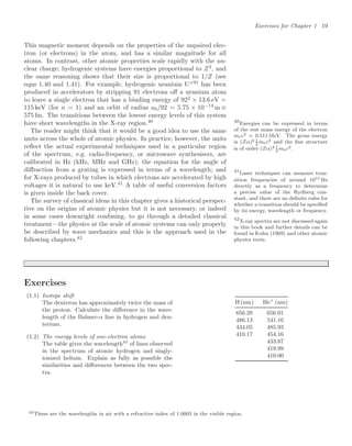
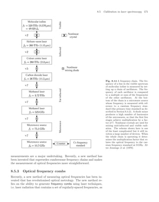
140. 7.1 Setting up the equations 125
Ω =
eX12|E0|
, (7.12)
where
X12 = 1| x |2 . (7.13)
To solve the coupled differential equations for c1 (t) and c2 (t) we need
to make further approximations.
7.1.2 The rotating-wave approximation
When all the population starts in the lower level, c1 (0) = 1 and c2 (0) =
0, integration of eqns 7.9 and 7.10 leads to
c1 (t) = 1 ,
c2 (t) =
Ω
2
∗
1 − exp [i(ω0 + ω)t]
ω0 + ω
+
1 − exp [i(ω0 − ω)t]
ω0 − ω
.
(7.14)
This gives a reasonable first-order approximation while c2 (t) remains
small. For most cases of interest, the radiation has a frequency close to
the atomic resonance at ω0 so the magnitude of the detuning is small,
|ω0 − ω| ω0, and hence ω0 + ω ∼ 2ω0. Therefore we can neglect the
term with denominator ω0 + ω inside the curly brackets. This is the
rotating-wave approximation.5
The modulus-squared of the co-rotating 5
This is not true for the interaction of
atoms with radiation at 10.6 µm from a
CO2 laser. This laser radiation has a
frequency closer to d.c. than to the res-
onance frequency of the atoms, e.g. for
rubidium with a resonance transition in
the near infra-red (780 nm) we find that
ω0 15ω, hence ω0 +ω ω0 −ω. Thus
the counter-rotating term must be kept.
The quasi-electrostatic traps (QUEST)
formed by such long wavelength laser
beams are a form of the dipole-force
traps described in Chapter 10.
term gives the probability of finding the atom in the upper state at time
t as
|c2 (t)|
2
=
Ω
sin {(ω0 − ω)t/2}
ω0 − ω
2
, (7.15)
or, in terms of the variable x = (ω − ω0)t/2,
|c2 (t)|
2
=
1
4
|Ω|
2
t2 sin2
x
x2
. (7.16)
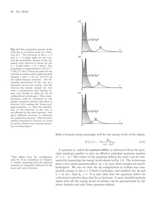
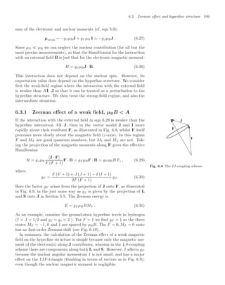
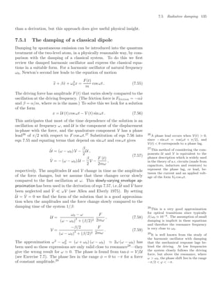
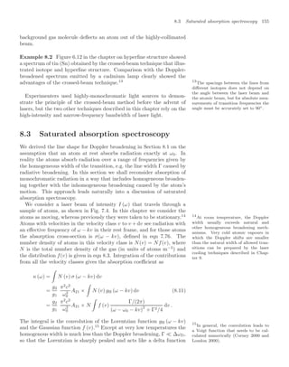
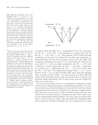
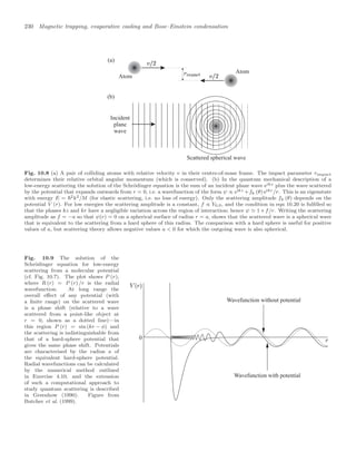
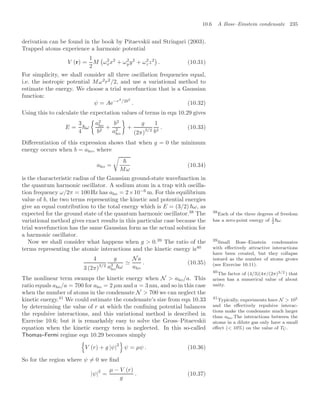
The sinc function (sin x) /x has a maximum at x = 0, and the first
minimum occurs at x = π or ω0 − ω = ±2π/t, as illustrated in Fig. 7.1;
the frequency spread decreases as the interaction time t increases.
Fig. 7.1 The excitation probability
function of the radiation frequency has
a maximum at the atomic resonance.
The line width is inversely proportional
to the interaction time. The function
sinc2 also describes the Fraunhofer dif-
fraction of light passing through a sin-
gle slit—the diffraction angle decreases
as the width of the aperture increases.
The mathematical correspondence be-
tween these two situations has a natural
explanation in terms of Fourier trans-
forms.

141. 126 The interaction of atoms with radiation
7.2 The Einstein B coefficients
In the previous section we found the effect of an electric field E0 cos (ωt)
on the atom. To relate this to Einstein’s treatment of the interaction
with broadband radiation we consider what happens with radiation of
energy density ρ (ω) in the frequency interval ω to ω+dω. This produces
an electric field of amplitude E0 (ω) given by ρ (ω) dω = 0E2
0 (ω) /2.
For this narrow (almost monochromatic) slice of the broad distribution
eqn 7.12 gives
|Ω|2
=
eX12E0 (ω)
2
=
e2
|X12|2
2
2ρ (ω) dω
0
. (7.17)
Integration of eqn 7.15 over frequency gives the excitation probability
for the broadband radiation as
|c2 (t)|
2
=
2e2
|X12|
2
02
ω0+∆/2
ω0−∆/2
ρ (ω)
sin2
{(ω0 − ω)t/2}
(ω0 − ω)2 dω . (7.18)
We integrate the squares of the amplitudes, rather than taking the square
of the total amplitude, since contributions at different frequencies do
not interfere.6
The range of integration ∆ must be large compared to
6
As in optics experiments with broad-
band light, it is intensities that are
summed, e.g. the formation of white-
light fringes in the Michelson interfer-
ometer.
the extent of the sinc function, but this is easily fulfilled since as time
increases this function becomes sharply peaked at ω0. (In the limit
t → ∞ it becomes a Dirac delta function—see Loudon (2000).) Over
the small range about ω0 where the sinc function has an appreciable
value, a smooth function like ρ (ω) varies little, so we take ρ (ω0) outside
the integral. A change of variable to x = (ω − ω0) t/2, as in eqn 7.16,
leads to
|c2 (t)|2
2e2
|X12|2
02
ρ (ω0) ×
t
2
+φ
−φ
sin2
x
x2
dx . (7.19)
The integration has limits of x = ±φ = ±∆t/4 π and the integral ap-
proximates closely to
∞
−∞
x−2
sin2
x dx = π. We make this assumption
of a long interaction to find the steady-state excitation rate for broad-
band radiation. The probability of transition from level 1 to 2 increases
linearly with time corresponding to a transition rate of
R12 =
|c2 (t)|
2
t
=
πe2
|X12|
2
02
ρ (ω0) . (7.20)
Comparison with the upward rate B12ρ (ω) in Einstein’s treatment of
radiation (eqn 1.25) shows that
B12 =
πe2
|D12|
2
302
, (7.21)
where |X12|
2
→ |D12|
2
/3, and D12 is the magnitude of the vector
D12 = 1| r |2 ≡
ψ∗
1 r ψ2 d3
r . (7.22)

142. 7.3 Interaction with monochromatic radiation 127
The factor of 1/3 arises from averaging of D ·
erad, where
erad is a unit
vector along the electric field, over all the possible spatial orientations
of the atom (see Exercise 7.6). The relation between A21 and B12 in
eqn 1.32 leads to
A21 =
g1
g2
4α
3c2
× ω3
|D12|2
, (7.23)
where α = e2
/ (4π0c) is the fine-structure constant. The matrix ele-
ment between the initial and final states in eqn 7.22 depends on an inte-
gral involving the electronic wavefunctions of the atom so, as emphasised
previously, the Einstein coefficients are properties of the atom. For a typ-
ical allowed transition the matrix element has an approximate value of
D12 3a0 (this can be calculated analytically for hydrogenic systems).
Using this estimate of D12 in the equation gives A21 2π × 107
s−1
for
a transition of wavelength λ = 6 × 10−7
m and g1 = g2 = 1. Although
we have not given a physical explanation of spontaneous emission, Ein-
stein’s argument allows us to calculate its rate; he obtained the relation
between A21 and B21 and we have used TDPT to determine B21 from the
atomic wavefunctions. For a two-level atom with an allowed transition
between the levels the quantum mechanical result corresponds closely
to the treatment of radiative decay using classical electromagnetism in
Section 1.6.
7.3 Interaction with monochromatic
radiation
The derivation of eqns 7.14 assumed that the monochromatic radiation
perturbed the atom only weakly so that most of the population stayed
in the initial state. We shall now find a solution without assuming a
weak field. We write eqn 7.9 as
i
.
c1 = c2
(
ei(ω−ω0)t
+ e−i(ω+ω0)t
) Ω
2
, (7.24)
and similarly for eqn 7.10. The term with (ω + ω0) t oscillates very fast
and therefore averages to zero over any reasonable interaction time—this
is the rotating-wave approximation (Section 7.1.2) and it leads to
i
.
c1 = c2ei(ω−ω0)t Ω
2
,
i
.
c2 = c1e−i(ω−ω0)t Ω∗
2
.
(7.25)
These combine to give
d2
c2
dt2
+ i (ω − ω0)
dc2
dt
+
Ω
2
2
c2 = 0 . (7.26)
The solution of this second-order differential equation for the initial con-
ditions c1 (0) = 1 and c2 (0) = 0 gives the probability of being in the
upper state as7
7
For transitions between bound states
the frequency Ω is real, so |Ω|2
= Ω2.

143. 128 The interaction of atoms with radiation
|c2 (t)|
2
=
Ω2
W2
sin2
Wt
2
, (7.27)
where
W2
= Ω2
+ (ω − ω0)2
. (7.28)
At resonance ω = ω0 and W = Ω, so
|c2 (t)|2
= sin2
Ωt
2
. (7.29)
The population oscillates between the two levels. When Ωt = π all the
population has gone from level 1 into the upper state, |c2 (t)|2
= 1, and
when Ωt = 2π the atom has returned to the lower state. This behaviour
is completely different from that of a two-level system governed by rate
equations where the populations tend to become equal as the excitation
rate increases and population inversion cannot occur. These Rabi os-
cillations between the two levels are readily observed in radio-frequency
spectroscopy, e.g. for transitions between Zeeman or hyperfine states.
Radio-frequency and microwave transitions have negligible spontaneous
emission so that, in most cases, the atoms evolve coherently.8
8
This is partly a consequence of the
dependence on ω3 in eqn 7.23, but
also because the magnetic dipole transi-
tions have smaller matrix elements than
electric dipole transitions. For electric
dipole transitions in the optical region
spontaneous emission washes out the
Rabi oscillations on a time-scale of tens
of nanoseconds (τ = 1/A21, assuming
that the predominant decay is from 2
to 1, and we estimated A12 above).
Nevertheless, experimenters have ob-
served coherent oscillations by driving
the transition with intense laser radi-
ation to give a high Rabi frequency
(Ωτ 1).
7.3.1 The concepts of π-pulses and π/2-pulses
A pulse of resonant radiation that has a duration of tπ = π/Ω is called
a π-pulse and from eqn 7.29 we see that Ωt = π results in the complete
transfer of population from one state to the other, e.g. an atom initially
in |1 ends up in |2 after the pulse. This contrasts with illumination by
broadband radiation where the populations (per state) become equal as
the energy density ρ (ω) increases. More precisely, a π-pulse swaps the
states in a superposition:9
9
This can be shown by solving
eqns 7.25 (and 7.26) for ω = ω0.
c1 |1 + c2 |2 → −i {c1 |2 + c2 |1 } . (7.30)
This swap operation is sometimes also expressed as |1 ↔ |2 , but the
factor of −i is important in atom interferometry, as shown in Exer-
cise 7.3.
Interferometry experiments also use π/2-pulses that have half the du-
ration of a π-pulse (for the same Rabi frequency Ω). For an atom initially
in state |1 , the π/2-pulse puts its wavefunction into a superposition of
states |1 and |2 with equal amplitudes (see Exercise 7.3).
7.3.2 The Bloch vector and Bloch sphere
In this section we find the electric dipole moment induced on a atom by
radiation, and introduce a very powerful way of describing the behaviour
of two-level systems by the Bloch vector. We assume that the electric
field is along
ex, as in eqn 7.12. The component of the dipole along this
direction is given by the expectation value
−eDx(t) = −
Ψ†
(t) ex Ψ(t) d3
r . (7.31)

144. 7.3 Interaction with monochromatic radiation 129
Using eqn 7.5 for Ψ (t) gives this dipole moment of the atom as
Dx(t) =
c1e−iω1t
ψ1 + c2e−iω2t
ψ2
∗
x
c1e−iω1t
ψ1 + c2e−iω2t
ψ2
d3
r
= c∗
2c1X21eiω0t
+ c∗
1c2X12e−iω0t
. (7.32)
Here ω0 = ω2 − ω1. The dipole moment is a real quantity since from
eqn 7.13 we see that X21 = (X12)∗
, and also X11 = X22 = 0. To calculate
this dipole moment induced by the applied field we need to know the
bilinear quantities c∗
1c2 and c∗
2c1. These are some of the elements of the
density matrix10 10
This is the outer product of |Ψ and
its Hermitian conjugate Ψ| ≡ |Ψ†
, the
transposed conjugate of the matrix rep-
resenting |Ψ. This way of writing the
information about the two levels is an
extremely useful formalism for treating
quantum systems. However, we have no
need to digress into the theory of den-
sity matrices here and we simply adopt
it as a convenient notation.
|Ψ Ψ| =
c1
c2
c∗
1 c∗
2
=
1
|c1|
2
c1c∗
2
c2c∗
1 |c2|
2
2
=
ρ11 ρ12
ρ21 ρ22
. (7.33)
Off-diagonal elements of the density matrix are called coherences and
they represent the response of the system at the driving frequency (eqn
7.32). The diagonal elements |c1|
2
and |c2|
2
are the populations. We
define the new variables
%
c1 = c1e−iδt/2
, (7.34)
%
c2 = c2eiδt/2
, (7.35)
where δ = ω − ω0 is the detuning of the radiation from the atomic
resonance. This transformation does not affect the populations ( %
ρ11 =
ρ11 and %
ρ22 = ρ22) but the coherences become %
ρ12 = ρ12 exp(−iδt) and
%
ρ21 = ρ21 exp(iδt) = (%
ρ12)∗
. In terms of these coherences the dipole
moment is11 11
We assume that X12 is real. This is
true for transitions between two bound
states of the atom—the radial wave-
functions are real and the discussion
of selection rules shows that the in-
tegration over the angular momentum
eigenfunctions also gives a real contri-
bution to the matrix element—the in-
tegral over φ is zero unless the terms
containing powers of exp(−iφ) cancel.
−eDx (t) = −eX12
ρ12eiω0t
+ ρ21e−iω0t
= −eX12
%
ρ12eiωt
+ %
ρ21e−iωt
= −eX12 (u cos ωt − v sin ωt) . (7.36)
The coherences %
ρ12 and %
ρ21 give the response of the atom at ω, the
(angular) frequency of the applied field. The real and imaginary parts
of %
ρ12 (multiplied by 2) are:
u = %
ρ12 + %
ρ21 ,
v = −i (%
ρ12 − %
ρ21) .
(7.37)
In eqn 7.36 we see that u and v are the in-phase and quadrature com-
ponents of the dipole in a frame rotating at ω. To find expressions for
%
ρ12, %
ρ21 and ρ22, and hence u and v, we start by writing eqns 7.25 for
c1 and c2 in terms of δ as follows:12 12
All the steps in this lengthy proce-
dure cannot be written down here but
enough information is given for metic-
ulous readers to fill in the gaps.
i
.
c1 = c2eiδt Ω
2
, (7.38)
i
.
c2 = c1e−iδt Ω
2
. (7.39)
Differentiation of eqn 7.34 yields13
13
Spontaneous decay is ignored here—
this section deals only with coherent
evolution of the states.

145. 130 The interaction of atoms with radiation
.
%
c1 =
.
c1e−iδt/2
−
iδ
2
c1e−iδt/2
. (7.40)
Multiplication by i and the use of eqns 7.38, 7.34 and 7.35 yields an
equation for
.
%
c1 (and similarly we can obtain
.
%
c2 from eqn 7.39):
i
.
%
c1 =
1
2
(δ %
c1 + Ω %
c2) ,
i
.
%
c2 =
1
2
(Ω %
c1 − δ %
c2) .
(7.41)
From these we find that the time derivatives
.
%
ρ12 = %
c1
.
%
c
∗
2 +
.
%
c1%
c
∗
2, etc. are
d%
ρ12
dt
=
d%
ρ21
dt
∗
= −iδ %
ρ12 +
iΩ
2
(ρ11 − ρ22) ,
dρ22
dt
= −
dρ11
dt
=
iΩ
2
(%
ρ21 − %
ρ12) .
(7.42)
The last equation is consistent with normalisation in eqn 7.7, i.e.
ρ22 + ρ11 = 1 . (7.43)
In terms of u and v in eqns 7.37 these equations become
.
u = δ v ,
.
v = −δ u + Ω (ρ11 − ρ22) ,
.
ρ22 =
Ωv
2
.
(7.44)
We can write the population difference ρ11 − ρ22 as14
14
This is appropriate for calculating
absorption. Alternatively, ρ22 − ρ11
could be chosen as a variable—this pop-
ulation inversion determines the gain in
lasers.
w = ρ11 − ρ22 , (7.45)
so that finally we get the following compact set of equations:
.
u = δ v ,
.
v = −δ u + Ωw ,
.
w = −Ωv .
(7.46)
These eqns 7.46 can be written in vector notation as:
.
R = R × (Ω
e1 + δ
e3) = R × W , (7.47)
by taking u, v and w as the components of the Bloch vector
R = u
e1 + v
e2 + w
e3 , (7.48)
and defining the vector
W = Ω
e1 + δ
e3 (7.49)
that has magnitude W =
√
Ω2 + δ2 (cf. eqn 7.28). The cross-product of
the two vectors in eqn 7.47 is orthogonal to both R and W. This implies

146. 7.3 Interaction with monochromatic radiation 131
that
.
R · R = 0 so |R|
2
is constant—it is straightforward15
to show that 15
|R| = 1 for the state u = v = 0, w =
1 and it always remains unity. This can
also be proved by writing u, v and w in
terms of |c1|2
, |c2|2
, etc.
this constant is unity so that |R|
2
= |u|
2
+ |v|
2
+ |w|
2
= 1. The Bloch
vector corresponds to the position vector of points on the surface of a
sphere with unit radius; this Bloch sphere is shown in Fig. 7.2.
It also follows from eqn 7.47 that
.
R · W = 0 and so R·W = RW cos θ
is constant. For excitation with a fixed Rabi frequency and detuning
the magnitude W is constant, and since R is also fixed the Bloch vector
moves around a cone with θ constant, as illustrated in Fig. 7.2(d). In
this case ρ22 varies as in eqn 7.27 and
w = 1 − 2ρ22 = 1 −
2Ω2
W2
sin2
Wt
2
.
This motion of the Bloch vector for the state of the atom resembles that
of a magnetic moment in a magnetic field,16
e.g. for adiabatic motion the
16
As described in Blundell (2001, Ap-
pendix G).
(a) (b)
(c) (d)
Fig. 7.2 The Bloch sphere. The position vectors of points on its surface represent the states of a two-level system (in
Hilbert space). Examples of states are shown in (a) and (b). At the poles of the sphere the Bloch vector is R = w
e3, with
w = ±1 corresponding to the states |1 and |2, respectively. States that lie on the equator of the Bloch sphere have the
form R = u
e1 + v
e2, e.g. the states for which R = v
e2 with u = 0 and v = ±1 are shown in (b) and these correspond
to (|1 ± i |2)/
√
2, respectively (normalisation constants are not given in the figure for clarity). These examples illustrate an
interesting property of this representation of quantum states, namely that diametrically-opposite states on the Bloch sphere
are orthogonal. (c) The evolution of the Bloch vector for a system driven by a resonant field, i.e. δ = 0 so that W = Ω
e1 in
eqn 7.49. The evolution follows a great circle from |1 at the north pole to |2 at the south pole and back again, as described
in Example 7.1. The Bloch vector remains perpendicular to W. (d) When δ = 0 the Bloch vector also has a fixed angle with
respect to W, since R · W = RW cos θ is constant, but θ is not equal to π/2. (This quantum mechanical description of the
two-level atom is equivalent to that for a spin-1/2 system.)

147. 132 The interaction of atoms with radiation
energy −µ · B is constant, and the magnetic moment precesses around
the direction of the field B = B
ez. In the Bloch description the fictitious
magnetic field lies along W and the magnitude W in eqn 7.28 determines
the precession rate.
Example 7.1 Resonant excitation (δ = 0) gives W = Ω
e1 and R
describes a cone about
e1. An important case is when all the population
starts in level 1 so that initially R ·
e1 = 0; in this case the Bloch vector
rotates in the plane perpendicular to
e1 mapping out a great circle on
the Bloch sphere, as drawn in Fig. 7.2(c). This motion corresponds to
the Rabi oscillations (eqn 7.29). In this picture a π/2-pulse rotates the
Bloch vector through π/2 about
e1. A sequence of two π/2-pulses gives
a π-pulse that rotates the Bloch vector (clockwise) through π about
e1, e.g. w = 1 → w = −1 and this represents the transfer of all the
population from level 1 to 2.17
This is consistent with the more general
17
In this particular example the fi-
nal state is obvious by inspection, but
clearly the same principles apply to
other initial states, e.g. states of the
form
|1 + eiφ |2
/
√
2 that lie on the
equator of the sphere. The Bloch
sphere is indispensable for thinking
about more complex pulse sequences,
such as those used in nuclear magnetic
resonance (NMR).
statement given in eqn 7.30.
The very brief introduction to the Bloch sphere given in this section
shows clearly that a two-level atom’s response to radiation does not
increase indefinitely with the driving field—beyond a certain point an
increase in the applied field (or the interaction time) does not produce
a larger dipole moment or change in population. This ‘saturation’ has
important consequences and makes the two-level system different from a
classical oscillator (where the dipole moment is proportional to the field,
as will be shown in Section 7.5).
7.4 Ramsey fringes
The previous sections in this chapter have shown how to calculate the
response of a two-level atom to radiation. In this section we shall apply
this theory to radio-frequency spectroscopy, e.g. the method of magnetic
resonance in an atomic beam described in Chapter 6. However, the same
principles are important whenever line width is limited by the finite
interaction time, both within atomic physics and more generally. In
particular, we shall calculate what happens to an atom subjected to two
pulses of radiation since such a double-pulse sequence has favourable
properties for precision measurements.
An atom that interacts with a square pulse of radiation, i.e. an os-
cillating electric field of constant amplitude from time t = 0 to τp, and
E0 = 0 otherwise, has a probability of excitation as in eqn 7.15.18
This
18
This assumes weak excitation:
|c2|2
1. excitation probability is plotted in Fig. 7.1 as a function of the radia-
tion’s frequency detuning from the (angular) resonance frequency ω0. As
stated below eqn 7.16, the frequency spread given by the first minimum
of the sinc2
function corresponds to a width19
19
This is not the FWHM but it is close
enough for our purposes.
∆f =
∆ω
2π
=
1
τp
. (7.50)
The frequency spread is inversely proportional to the interaction time,20
20
This expression is equivalent to
eqn 6.40 that was used to calculate the
line width for an atomic clock.

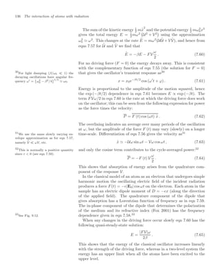
148. 7.4 Ramsey fringes 133
as expected from the Fourier transform relationship of the frequency and
time domains.
We shall now consider what happens when an atom interacts with two
separate pulses of radiation, from time t = 0 to τp and again from t = T
to T + τp. Integration of eqn 7.10 with the initial condition c2 = 0 at
t = 0 yields
c2 (t) =
Ω
2
∗
1 − exp[i(ω0 − ω)τp]
ω0 − ω
+ exp[i(ω0 − ω)T ]
1 − exp[i(ω0 − ω)τp]
ω0 − ω
.
(7.51)
This is the amplitude excited to the upper level after both pulses (t
T + τp). The first term in this expression is the amplitude arising from
the first pulse and it equals the part of eqn 7.14 that remains after
making the rotating-wave approximation.21
Within this approximation, 21
Neglecting terms with ω0 + ω in the
denominator.
interaction with the second pulse produces a similar term multiplied by
a phase factor of exp[i(ω0 −ω)T ]. Either of the pulses acting alone would
affect the system in the same way, i.e. the same excitation probability
|c2|
2
as in eqn 7.15. When there are two pulses the amplitudes in the
excited state interfere giving
|c2|
2
=
Ω
sin {(ω0 − ω)τp/2}
(ω0 − ω)
2
× |1 + exp[i(ω0 − ω)T ]|
2
=
Ωτp
2
2 3
sin (δ τp/2)
δ τp/2
42
cos2
δ T
2
, (7.52)
where δ = ω − ω0 is the frequency detuning. The double-pulse sequence
produces a signal of the form shown in Fig. 7.3. These are called Ramsey
fringes after Norman Ramsey and they have a very close similarity to the
interference fringes seen in a Young’s double-slit experiment in optics—
Fraunhofer diffraction of light with wavevector k from two slits of width
a and separation d leads to an intensity distribution as a function of
angle θ given by22 22
See Section 11.1 and Brooker (2003).
I = I0 cos2
1
2
kd sin θ
sinc2
1
2
ka sin θ
. (7.53)
The overall envelope proportional to sinc2
comes from single-slit diffrac-
tion. The cos2
function determines the width of the central peak in both
eqns 7.53 and 7.52.23 23
In both quantum mechanics and op-
tics, the amplitudes of waves inter-
fere constructively, or destructively, de-
pending on their relative phase. Also,
the calculation of Fraunhofer diffrac-
tion as a Fourier transform of ampli-
tude in the plane of the object closely
parallels the Fourier transform relation-
ship between pulses in the time domain
and the frequency response of the sys-
tem.
For the atom excited by two pulses of radiation the excitation drops
from the maximum value at ω = ω0 to zero when δ T/2 = π/2 (or to
half the maximum at π/4); so the central peak has a width (FWHM) of
∆ω = π/T , or equivalently
∆f =
1
2T
. (7.54)
This shows that Ramsey fringes from two interactions separated by time
T have half the width of the signal from a single long interaction of

149. 134 The interaction of atoms with radiation
Fig. 7.3 Ramsey fringes from an
atomic fountain of caesium, showing
the transition probability for the F = 3,
MF = 0 to F = 4, MF = 0 tran-
sition versus the frequency of the mi-
crowave radiation in the interaction re-
gion. The height of the fountain is
31 cm, giving a fringe width just be-
low 1 Hz (i.e. ∆f = 1/(2T) = 0.98 Hz,
see text)—the envelope of the fringes
has a more complicated shape than that
derived in the text, but this has lit-
tle influence since, during operation as
a frequency standard, the microwaves
have a frequency very close to the cen-
tre which, by definition, corresponds to
9 192 631 770 Hz. This is real experi-
mental data but the noise is not visi-
ble because the signal-to-noise ratio is
about 1000 (near the centre), and with
such an extremely high-quality signal
the short-term stability of a microwave
source referenced to the caesium tran-
sition is about 1 × 10−13 for 1 s of av-
eraging. Courtesy of Dale Henderson,
Krzysztof Szymaniec and Chalupczak
Witold, National Physical Laboratory,
Teddington, UK.
−80 −60 −40 −20 0
0.0
0.5
1.0
20 40 60 80
Transition
probability
Frequency of microwaves relative to line centre (Hz)
duration T (cf. eqn 7.50); also, it is often preferable to have two sepa-
rated interaction regions, e.g. for measurements in an atomic fountain
as described in Chapter 8.24
24
Ramsey originally introduced two
separated interactions in an atomic-
beam experiment to avoid the line
broadening by inhomogeneous mag-
netic fields. A small phase differ-
ence between the two interaction re-
gions just causes a phase shift of the
fringes, whereas if the atom interacts
with the radiation throughout a region
where the field varies then the contri-
butions from each part of the interac-
tion region do not add in phase. The
phasor description, commonly used in
optics, gives a good way of thinking
about this—Young’s fringes have a high
contrast when the two slits of separa-
tion d are illuminated coherently, but to
achieve the diffraction limit from a sin-
gle wide slit of width d requires a good
wavefront across the whole aperture.
In practice, microwave experiments use strong rather than weak exci-
tation (as assumed above) to obtain the maximum signal, i.e. |c2|
2
1.
This does not change the width of the Ramsey fringes, as shown by
considering two π/2-pulses separated by time T . If no phase shift ac-
cumulates between the two pulses they add together to act as a π-pulse
that transfers all the population to the upper state—from the north to
the south pole of the Bloch sphere, as shown in Fig. 7.2(c). But if a
relative phase shift of π accrues during the time interval T then there
is destructive interference between the amplitudes in the upper state
produced by the two pulses.25
Thus the first minimum from the central
25
In the Bloch sphere description this
corresponds to the following path: the
initial π/2-pulse causes
e3 →
e2, then
the accumulated phase causes the state
vector to move around the equator of
the sphere to −
e2, from whence the fi-
nal π/2-pulse takes the system back up
to
e3 (see Fig. 7.2). This formalism al-
lows quantitative calculation of the fi-
nal state for any type of pulse.
fringe occurs for δ T = π, which is the condition that gave eqn 7.54, and
so that equation remains accurate.
7.5 Radiative damping
This section shows how damping affects the coherent evolution of the
Bloch vector described in the previous section. It is shown by analogy
with the description of a classical dipole that a damping term should be
introduced into eqns 7.46. Ultimately, such an argument by analogy is
only a justification that the equations have an appropriate form rather

150. 7.5 Radiative damping 135
than a derivation, but this approach does give useful physical insight.
7.5.1 The damping of a classical dipole
Damping by spontaneous emission can be introduced into the quantum
treatment of the two-level atom, in a physically reasonable way, by com-
parison with the damping of a classical system. To do this we first
review the damped harmonic oscillator and express the classical equa-
tions in a suitable form. For a harmonic oscillator of natural frequency
ω0, Newton’s second law leads to the equation of motion
..
x + β
.
x + ω2
0x =
F(t)
m
cos ωt . (7.55)
The driving force has amplitude F(t) that varies slowly compared to the
oscillation at the driving frequency. (The friction force is Ffriction = −α
.
x
and β = α/m, where m is the mass.) To solve this we look for a solution
of the form
x = U (t) cos ωt − V (t) sin ωt . (7.56)
This anticipates that most of the time dependence of the solution is an
oscillation at frequency ω, and U is the component of the displacement
in-phase with the force, and the quadrature component V has a phase
lead26
of π/2 with respect to F cos ωt.27
Substitution of eqn 7.56 into 26
A phase lead occurs when V(t) 0,
since − sin ωt = cos(ωt + π/2), and
V(t) 0 corresponds to a phase lag.
27
This method of considering the com-
ponents U and V is equivalent to the
phasor description which is widely used
in the theory of a.c. circuits (made from
capacitors, inductors and resistors) to
represent the phase lag, or lead, be-
tween the current and an applied volt-
age of the form V0 cos ωt.
eqn 7.55 and equating terms that depend on sin ωt and cos ωt gives
.
U = (ω − ω0) V −
β
2
U ,
.
V = − (ω − ω0) U −
β
2
V −
F (t)
2mω
,
(7.57)
respectively. The amplitudes U and V change in time as the amplitude
of the force changes, but we assume that these changes occur slowly
compared to the fast oscillation at ω. This slowly-varying envelope ap-
proximation has been used in the derivation of eqn 7.57, i.e.
..
U and
..
V have
been neglected and
.
V ωV (see Allen and Eberly 1975). By setting
.
U =
.
V = 0 we find the form of the solution that is a good approxima-
tion when the amplitudes and the force change slowly compared to the
damping time of the system 1/β:
U =
ω0 − ω
(ω − ω0)
2
+ (β/2)2
F
2mω
, (7.58)
V =
−β/2
(ω − ω0)
2
+ (β/2)2
F
2mω
. (7.59)
The approximation ω2
− ω2
0 = (ω + ω0) (ω − ω0) 2ω (ω − ω0) has
been used so these expressions are only valid close to resonance28
—they
28
This is a very good approximation
for optical transitions since typically
β/ω0 10−6. The assumption of small
damping is implicit in these equations
and therefore the resonance frequency
is very close to ω0.
give the wrong result for ω 0. The phase is found from tan φ = V/U
(see Exercise 7.7). The phase lies in the range φ = 0 to −π for a force
of constant amplitude.29
29
It is well known from the study of
the harmonic oscillator with damping
that the mechanical response lags be-
hind the driving. At low frequencies
the system closely follows the driving
force, but above the resonance, where
ω ω0, the phase shift lies in the range
−π/2 ϕ −π.

151. 136 The interaction of atoms with radiation
The sum of the kinetic energy 1
2 m
.
x
2
and the potential energy 1
2 mω2
0x2
gives the total energy E = 1
2 mω2
U2
+ V2
using the approximation
ω2
0 ω2
. This changes at the rate
.
E = mω2
(U
.
U + V
.
V), and hence from
eqns 7.57 for
.
U and
.
V we find that
.
E = −βE − FV
ω
2
. (7.60)
For no driving force (F = 0) the energy decays away. This is consistent
with the complementary function of eqn 7.55 (the solution for F = 0)
that gives the oscillator’s transient response as30
30
For light damping (β/ω0 1) the
decaying oscillations have angular fre-
quency ω =
ω2
0 − β2/4
1/2
ω0. x = x0e−βt/2
cos (ω
t + ϕ) . (7.61)
Energy is proportional to the amplitude of the motion squared, hence
the exp (−βt/2) dependence in eqn 7.61 becomes E ∝ exp (−βt). The
term FVω/2 in eqn 7.60 is the rate at which the driving force does work
on the oscillator; this can be seen from the following expression for power
as the force times the velocity:
P = F (t) cos (ωt)
.
x . (7.62)
The overlining indicates an average over many periods of the oscillation
at ω, but the amplitude of the force F (t) may vary (slowly) on a longer
time-scale. Differentiation of eqn 7.56 gives the velocity as31
31
We use the same slowly varying en-
velope approximation as for eqn 7.57,
namely
.
V ωV, etc.
.
x −Uω sin ωt − Vω cos ωt , (7.63)
and only the cosine term contributes to the cycle-averaged power:32
32
This is normally a positive quantity
since r 0 (see eqn 7.59).
P = −F (t) V
ω
2
. (7.64)
This shows that absorption of energy arises from the quadrature com-
ponent of the response V.
In the classical model of an atom as an electron that undergoes simple
harmonic motion the oscillating electric field of the incident radiation
produces a force F(t) = −e|E0| cos ωt on the electron. Each atom in the
sample has an electric dipole moment of D = −ex (along the direction
of the applied field). The quadrature component of the dipole that
gives absorption has a Lorentzian function of frequency as in eqn 7.59.
The in-phase component of the dipole that determines the polarization
of the medium and its refractive index (Fox 2001) has the frequency
dependence given in eqn 7.58.33
33
See Fig. 9.12.
When any changes in the driving force occur slowly eqn 7.60 has the
following quasi-steady-state solution:
E =
|FV|ω
2β
. (7.65)
This shows that the energy of the classical oscillator increases linearly
with the strength of the driving force, whereas in a two-level system the
energy has an upper limit when all the atoms have been excited to the
upper level.

152. 7.5 Radiative damping 137
7.5.2 The optical Bloch equations
A two-level atom has an energy proportional to the excited-state pop-
ulation, E = ρ22ω0. By analogy with eqn 7.60 for the energy of a
classical oscillator, we introduce a damping term into eqn 7.44 to give
.
ρ22 = −Γρ22 +
Ω
2
v . (7.66)
In the absence of the driving term (Ω = 0) this gives exponential decay of
the population in level 2, i.e. ρ22(t) = ρ22(0) exp (−Γt). In this analogy,
between the quantum system and a classical oscillator, Γ corresponds to
β. From eqns 7.57 we see that the coherences u and v have a damping
factor of Γ/2 and eqns 7.46 become the optical Bloch equations34
34
The main purpose of the rather
lengthy discussion of the classical case
was to highlight the correspondence be-
tween u, v and U, V to make this step
seem reasonable. An auxiliary feature
of this approach is to remind the reader
of the classical electron oscillator model
of absorption and dispersion (which is
important in atomic physics).
.
u = δ v −
Γ
2
u ,
.
v = −δ u + Ωw −
Γ
2
v ,
.
w = −Ωv − Γ (w − 1) .
(7.67)
For Ω = 0 the population difference w → 1. These optical Bloch equa-
tions describe the excitation of a two-level atom by radiation close to
resonance for a transition that decays by spontaneous emission. There
is not room here to explore all of the features of these equations and
their many diverse and interesting applications; we shall concentrate
on the steady-state solution that is established at times which are long
compared to the lifetime of the upper level (t Γ−1
), namely35
35
The steady-state solution is obtained
by setting
.
u =
.
v =
.
w = 0 in eqns 7.67
to give three simultaneous equations.


u
v
w

 =
1
δ2 + Ω2/2 + Γ2/4


Ω δ
Ω Γ/2
δ2
+ Γ2
/4

 . (7.68)
These show that a strong driving field (Ω → ∞) tends to equalise the
populations, i.e. w → 0. Equivalently, the upper level has a steady-state
population of
ρ22 =
1 − w
2
=
Ω2
/4
δ2 + Ω2/2 + Γ2/4
, (7.69)
and ρ22 → 1/2 as the intensity increases. This key result is used in
Chapter 9 on radiation forces.
In the above, the optical Bloch equations have been justified by anal-
ogy with a damped classical oscillator but they also closely resemble the
Bloch equations that describe the behaviour of a spin-1/2 particle in a
combination of static and oscillating magnetic fields.36
The reader fa-
36
The Zeeman effect leads to a split-
ting between states with ms = ±1/2
to give a two-level system, and the os-
cillating magnetic field drives magnetic
dipole transitions between the levels. In
atomic physics such transitions occur
between Zeeman states and hyperfine
levels (Chapter 6).
miliar with magnetic resonance techniques may find it useful to make an
analogy with that historically important case.37
For times much shorter
37
The Bloch equations were well known
from magnetic resonance techniques
before lasers allowed the observation
of coherent phenomena in optical tran-
sitions. Radio-frequency transitions
have negligible spontaneous emission
and the magnetic dipole of the whole
sample decays by other mechanisms.
Where the optical Bloch equations
(eqns 7.67) have decay constants of Γ
and Γ/2 for the population and co-
herences, respectively, the Bloch equa-
tions have 1/T1 and 1/T2. The de-
cay rates 1/T1 and 1/T2 in magnetic
resonance techniques are expressed in
terms of T1 and T2, the longitudinal
and transverse relaxation times, respec-
tively. Under some conditions the two
relaxation times are similar, but in
other cases T2 T1. T1 describes
the relaxation of the component of the
magnetic moment parallel to the ap-
plied field B which requires exchange
of energy (e.g. with the phonons in a
solid). T2 arises from the dephasing of
individual magnetic moments (spins) so
that the magnetisation of the sample
perpendicular to B decays. For further
details see condensed matter texts, e.g.
Kittel (2004).
than any damping or relaxation time, the two-level atom and spin-1/2
system behave in the same way, i.e. they have a coherent evolution such
as π- and π/2-pulses, etc. A steady-state solution of the optical Bloch
equations has been presented (and nothing has been said about the dif-
ferent result for a spin-1/2 system).

153. 138 The interaction of atoms with radiation
7.6 The optical absorption cross-section
Monochromatic radiation causes an atom to undergo Rabi oscillations,
but when the transition has damping the atom settles down to a steady
state in which the excitation rate equals the decay rate. This has been
shown explicitly above for an optical transition with spontaneous emis-
sion, but the same reduction of the coherent evolution of quantum am-
plitudes to a simple rate equation for populations (amplitudes squared)
also occurs for other line-broadening mechanisms, e.g. Doppler broad-
ening (Chapter 8) and collisions. Thus the equilibrium situation for
monochromatic radiation is described by rate equations like those in
Einstein’s treatment of excitation by broadband radiation (eqns 1.25).
It is convenient to write these rate equations in terms of an optical ab-
sorption cross-section defined in the usual way, as in Fig. 7.4. Consider a
beam of particles (in this case photons) passing through a medium with
N atoms per unit volume.38
A slab of thickness ∆z has N∆z atoms per
38
N represents the number density and
has dimensions of m−3, following the
usual convention in laser physics.
unit area and the fraction of particles absorbed by the target atoms is
Nσ∆z, where σ is defined as the cross-section; Nσ∆z gives the fraction
of the target area covered by the atoms and this equals the probabil-
ity that an incident particle hits an atom in the target (as it passes
through the slab). The parameter σ that characterises the probability
of absorption is equally well definable in quantum mechanics (in which
photons and particles are delocalised, fuzzy objects) even though this
cross-section generally has little relation to the physical size of the ob-
ject (as we shall see). The probability of absorption equals the fraction
of intensity lost, ∆I/I = −Nσ∆z, so the attenuation of the beam is
described by
dI
dz
= −κ (ω) I = −Nσ(ω)I , (7.70)
where κ (ω) is the absorption coefficient at the angular frequency ω of
the incident photons. Integration gives an exponential decrease of the
intensity with distance, namely
I (ω, z) = I (ω, 0) exp {−κ (ω) z} . (7.71)
Fig. 7.4 Atoms with number density
N distributed in a slab of thickness ∆z
absorb a fraction Nσ∆z of the inci-
dent beam intensity, where σ is defined
as the cross-section (for absorption).
N∆z is the number of atoms per unit
area and σ represents the ‘target’ area
that each atom presents. We assume
that the motion of the target atoms
can be ignored (Doppler broadening is
treated in Exercise 7.9) and also that
atoms in the next layer (of thickness
δz) cannot ‘hide’ behind these atoms
(see Brooker 2003, Problem 3.26).

154. 7.6 The optical absorption cross-section 139
This formula, known as Beer’s law (see Fox 2001), works well for ab-
sorption of low-intensity light that leaves most of the population in the
ground state. Intense laser light significantly affects the populations of
the atomic levels and we must take this into account. Atoms in level 2
undergo stimulated emission and this process leads to a gain in intensity
(amplification) that offsets some of the absorption. Equation 7.70 must
be modified to39 39
We do not try to include the degen-
eracy of the levels because illumination
with intense polarized laser light usu-
ally leads to unequal populations of the
states with different MJ , or MF . This
differs from the usual situation in laser
physics where the excitation, or pump-
ing mechanisms, populate all states in a
given level at the same rate, so N1/g1
and N2/g2 can be taken as the pop-
ulation densities per state. Selective
excitation of the upper level can give
N2/g2 N1/g1, and hence gain.
dI
dz
= −κ (ω) I (ω) = −(N1 − N2)σ (ω) I (ω) . (7.72)
Absorption and stimulated emission have the same cross-section. For
the specific case of a two-level atom this can be seen from the symmetry
with respect to the exchange of the labels 1 and 2 in the treatment
of the two-level atom in the early parts of this chapter; the oscillating
electric field drives the transition from 1 to 2 at the same rate as the
reverse process—only the spontaneous emission goes one way. This is an
example of the general principle that a strong absorber is also a strong
emitter.40
This is also linked to the equality of the Einstein coefficients, 40
The laws of thermodynamics require
that an object stays in equilibrium with
black-body radiation at the same tem-
perature, hence the absorbed and emit-
ted powers must balance.
B12 = B21, for non-degenerate levels. The population densities in the
two levels obey the conservation equation N = N1 +N2.41
In the steady
41
Compare this with eqns 1.26, 7.7 and
7.43.
state conservation of energy per unit volume of the absorber requires
that
(N1 − N2)σ (ω) I (ω) = N2A21ω . (7.73)
On the left-hand side is the amount by which the rate of absorption
of energy exceeds the stimulated emission, i.e. the net rate of energy
absorbed per unit volume. On the right-hand side is the rate at which the
atoms scatter energy out of the beam—the rate of spontaneous emission
for atoms in the excited state times ω.42
The number densities are 42
This assumes that atoms do not get
rid of their energy in any other way
such as inelastic collisions.
related to the variables in the optical Bloch equations by ρ22 = N2/N
and
w =
N2 − N1
N
, (7.74)
and w and ρ22 are given in eqns 7.68 and 7.69, respectively. Hence
σ (ω) =
ρ22
w
A21ω
I
=
Ω2
/4
(ω − ω0)2
+ Γ2/4
×
A21ω
I
. (7.75)
Both I and Ω2
are proportional to |E0|
2
so this cancels out, and further
manipulation yields43 43
Intensity is related to the electric
field amplitude by I = 0c |E0 (ω)|2
/2,
and Ω2 = e2X2
12 |E0|2
/2 (eqn 7.12).
Also X2
12 = |D12|2
/3 ∝ A21 (eqn 7.23).
The degeneracy factors are g1 = g2 = 1
for the two-level atom, but see eqn 7.79.
σ (ω) = 3 ×
π2
c2
ω2
0
A21 gH (ω) . (7.76)
The Lorentzian frequency dependence is expressed by the line shape func-
tion
gH (ω) =
1
2π
Γ
(ω − ω0)
2
+ Γ2/4
, (7.77)
where the subscript H denotes homogeneous, i.e. something that is the
same for each atom, like the radiative broadening considered here.44
The
44
It is a general result that homoge-
neous broadening mechanisms give a
Lorentzian line shape.

155. 140 The interaction of atoms with radiation
area under this line shape function equals unity:
∞
−∞
gH (ω) dω = 1 . (7.78)
The pre-factor of 3 in eqn 7.76 may have any value in the range 0 to 3.
It has the maximum value of 3 for atoms with the optimum orientation
to absorb a beam of polarized laser light (from a specific direction).
However, if either the light is unpolarized or the atoms have a random
orientation (i.e. they are uniformly distributed across all the MJ states
or MF states) then the pre-factor is 1 because |X12|2
= |D12|2
/3 as
in eqn 7.21 (from the average of cos2
θ over all angles), and this 1/3
cancels the pre-factor of 3.45
Under these conditions the absorption does
45
Spontaneously emitted photons go in
random directions so an average over
angles always occurs in the calculation
of A21.
not depend on the magnetic state (MJ or MF ) so a real atom with
degenerate levels has a cross-section of
σ (ω) =
g2
g1
×
π2
c2
ω2
0
A21 gH (ω) . (7.79)
This equation, or eqn 7.76, applies to many experimental situations.
Careful study of the following examples gives physical insight that can
be applied to other situations.46
46
Typically, for atoms with a well-
defined orientation the polarization of
the light is chosen to give the maximum
cross-section. If this is not the case then
the angular momentum algebra may be
required to calculate the matrix ele-
ments. Only in special cases would the
polarization be chosen to give a very
weak interaction, i.e. a pre-factor much
less than unity in eqn 7.76.
Example 7.2 Atoms in a specific MF state interacting with a polarized
laser beam, e.g. sodium atoms in a magnetic trap that absorb a circularly-
polarized probe beam (Fig. 7.5)
This gives effectively a two-level system and the polarization of the light
matches the atom’s orientation so eqn 7.76 applies (the pre-factor has
the maximum value of 3). To drive the ∆MF = +1 transition the
a
b
c
Fig. 7.5 The Zeeman states of the 3s 2P1/2 F = 2 and 3p 2P3/2 F = 3 hyperfine
levels of sodium, and the allowed electric dipole transitions between them. The other
hyperfine levels (F = 1 and F = 0, 1 and 2) have not been shown. Excitation of the
transition F = 2, MF = 2 to F = 3, MF = 3 (labelled a) gives a closed cycle that
has similar properties to a two-level atom—the selection rules dictate that atoms in
the F = 3, MF = 3 state spontaneously decay back to the initial state. (Circularly-
polarized light that excites ∆MF = +1 transitions leads to cycles of absorption and
emission that tend to drive the population in the F = 2 level towards the state of
maximum MF , and this optical pumping process provides a way of preparing a sample
of atoms in this state.) When all the atoms have the correct orientation, i.e. they
are in the F = 2, MF = 2 state for this example, then eqn 7.76 applies. Atoms in
this state give less absorption for linearly-polarized light (transition b), or circular
polarization of the wrong handedness (transition c).

156. 7.6 The optical absorption cross-section 141
circularly-polarized light must have the correct handedness and propa-
gate along the atom’s quantisation axis (defined by the magnetic field
in this example).47 47
The direction of the electric field at
the atom depends on both the polar-
ization and direction of the radiation,
e.g. circularly-polarized light that prop-
agates perpendicular to the quantisa-
tion axis drives ∆MF = 0 and ±1
(π- and σ-) transitions. This leads to
a smaller cross-section than when the
light propagates along the axis. Radi-
ation that propagates in all directions
does not produce a polarized electric
field, e.g. isotropic radiation in a black-
body enclosure.
Example 7.3 The absorption of light on an s–p transition, e.g. the
3s–3p resonance line of sodium
Light with a particular polarization and direction drives a transition to
one magnetic sub-level in the upper level, as shown in Fig. 7.6(a). Since
the lower level has only ml = 0 there is no averaging over the orientation
and eqn 7.76 applies. Unpolarized light drives transitions to the three
upper ml states equally. For each transition the averaging gives a factor
of 1/3 but all three transitions contribute equally to the absorption so
the atoms have the same cross-section as for polarized light (eqn 7.79
with g2/g1 = 3). Thus the s–p transition is a special case that gives
the same absorption cross-section whatever the polarization of the light.
Atoms with ml = 0 have no preferred direction and interact in the same
way with light of any polarization (or direction). In contrast, for the p–s
transition shown in Fig. 7.6(b), atoms in a given ml state only interact
with light that has the correct polarization to drive the transition to
ml = 0.
48
Spin is ignored here. This applies
when either the fine structure is not re-
solved, e.g. this may arise for the tran-
sition 2s–3p in hydrogen where the fine
structure of the upper level is small,
or to transitions between singlet terms,
i.e. 1S–1P and 1P–1S (with ml → Ml
in the figure).
7.6.1 Cross-section for pure radiative broadening
The peak absorption cross-section given by eqn 7.76, when ω = ω0, is
σ (ω0) = 3 ×
2πc2
ω2
0
A21
Γ
. (7.80)
s p
p s
a b c e f g
(a) (b)
Fig. 7.6 A comparison of s–p and p–s transitions. (a) The three transitions a, b
and c between the s and p levels have equal strength. The physical reason for this is
that the spontaneous decay rate of the upper ml states cannot depend on the atom’s
orientation in space. Light linearly-polarized parallel to the z-axis drives π-transition
b only, and spontaneous decay occurs back to the initial state since there are no other
accessible states—this gives the equivalent of a two-level system. The s–p transition
is a special case where the absorption does not depend on the polarization, e.g.
unpolarized light gives equal excitation rates on the three transitions a, b and c, and
this increases the absorption by the degeneracy factor g2/g1 = 3, thereby cancelling
the 1/3 that arises in the orientational average. (b) In contrast, for the p–s transition
the peak cross-section is one-ninth of that in (a).48

157. 142 The interaction of atoms with radiation
In a two-level atom the upper level can only decay to level 1 so Γ = A21,
and for a transition of wavelength λ0 = 2πc/ω0 we find
σ (ω0) = 3 ×
λ2
0
2π
λ2
0
2
. (7.81)
This maximum cross-section is much larger than the size of the atom,
e.g. the λ0 = 589 nm transition of sodium has σ (ω0) = 2 × 10−13
m2
,
whereas in kinetic theory the atoms have a cross-section of only πd2
=
3×10−18
m−2
for an atomic diameter of d = 0.3 nm—‘collisions’ between
atoms and photons have a large resonant enhancement. The optical
cross-section decreases rapidly off resonance, e.g. light of wavelength
600 nm gives Γ/ (ω − ω0) = 10−6
for the sodium transition above, so
that σ (ω) = 10−12
× σ (ω0) = 2 × 10−25
m2
. Clearly the absorption of
radiation has little relation to the size of the electronic orbitals.
7.6.2 The saturation intensity
In the previous section we calculated the absorption cross-section start-
ing from eqn 7.73 and we shall now use the same equation to determine
the population difference; we can write eqn 7.73 as (N1 − N2) × r = N2,
where the dimensionless ratio r = σ (ω) I (ω) /(ωA21). This equation
and N1 + N2 = N give the difference in population densities as
N1 − N2 =
N
1 + 2r
=
N
1 + I/Is (ω)
, (7.82)
where the saturation intensity is defined by
Is (ω) =
ωA21
2σ (ω)
. (7.83)
It is important to note that other definitions of saturation intensity are
also used, such as the above expression without 2 in the denominator.
From eqn 7.72 we find that the absorption coefficient depends on inten-
sity as follows:49
49
This equation is very similar to the
formula for the saturation of gain in a
homogeneously-broadened laser system
since gain is negative absorption.
κ (ω, I) =
Nσ (ω)
1 + I/Is (ω)
. (7.84)
The minimum value of Isat (ω) occurs on resonance where the cross-
section is largest; this minimum value is often referred to as the satura-
tion intensity, Isat ≡ Is (ω0), given by50
50
Here Isat = ωA21/ (2σ(ω0)) and
σ(ω0) is given by eqn 7.81.
Isat =
π
3
hc
λ3τ
, (7.85)
where τ = Γ−1
is the lifetime for radiative broadening. For example, the
resonance transition in sodium at λ = 589 nm has a lifetime of τ = 16 ns
and for an appropriate polarization (as in Fig. 7.5) the atom cycles on
an effectively two-level transition. This leads to an intensity Isat =
60 W m−2
, or 6 mW cm−2
, that can easily be produced by a tunable dye
laser.

158. 7.6 The optical absorption cross-section 143
We can also obtain eqn 7.82 directly from the steady-state value of
w = (N1 − N2)/N in eqn 7.68 if the saturation intensity is defined by
I
Isat
=
2Ω2
Γ2
. (7.86)
This is equivalent to eqn 7.85.51
At saturation the Rabi frequency has a 51
As discussed after eqn 7.75, Ω2/I
does not depend on the electric field.
value comparable with Γ.
7.6.3 Power broadening
Equation 7.84 for κ (ω, I) contains two quantities that vary with fre-
quency: σ(ω) and Is(ω).52
Rearranging this equation to show the fre- 52
In terms of the minimum value
Isat = Is (ω0) we can rewrite eqn 7.83
as
Is (ω)
Isat
=
σ0
σ (ω)
.
We also have
σ (ω) = σ0
Γ2/4
(ω − ω0)2
+ Γ2/4
.
quency dependence, and defining σ0 ≡ σ(ω0) as the maximum cross-
section in eqn 7.81, we find that
κ (ω, I) = Nσ0
Γ2
/4
(ω − ω0)
2
+ Γ2/4
×
1
1 + I
Isat
Γ2/4
(ω−ω0)2
+Γ2/4
= Nσ0
Γ2
/4
(ω − ω0)
2
+ 1
4 Γ2 (1 + I/Isat)
. (7.87)
The expression for the absorption coefficient κ (ω, I) has a Lorentzian
line shape with a full width at half maximum (FWHM) of
∆ωFWHM = Γ
1 +
I
Isat
1/2
. (7.88)
The line width increases with intensity. This power broadening occurs
because saturation reduces the absorption near the resonance while far
from resonance the absorption changes little (see Fig. 7.7). The expres-
sion for the population in the upper level ρ22 in eqn 7.69 also has the
same power-broadened line width, as in eqn 7.88.53
The relationship be-
53
This can be shown by rearrangement
of the denominator of eqn 7.69 in terms
of a line width
∆ω = Γ
1 +
2Ω2
Γ2
1/2
= Γ
1 +
I
Isat
1/2
.
tween this absorption and the populations of the two levels is discussed
in Exercise 7.11.
Fig. 7.7 The absorption coefficient
κ(ω, I) is a Lorentzian function of the
frequency that peaks at ω0, the atomic
resonance. Saturation causes the ab-
sorption line shape to change from the
curve for a low intensity (I Isat,
dashed line), to a broader curve (solid
line), with a lower peak value, described
by the Lorentzian function in eqn 7.87.

159. 144 The interaction of atoms with radiation
7.7 The a.c. Stark effect or light shift
In addition to its effect on the populations, the perturbing radiation also
changes the energy of the levels and we calculate this light shift in this
section. We can write eqns 7.41 for %
c1 and %
c2 in matrix form as
i
d
dt
%
c1
%
c2
=
δ/2 Ω/2
Ω/2 −δ/2
%
c1
%
c2
. (7.89)
This has solutions of the form
%
c1
%
c2
=
a
b
e−iλt
. (7.90)
The equation for the eigenvalues λ is
δ/2 − λ Ω/2
Ω/2 −δ/2 − λ
= λ2
−
δ
2
2
−
Ω
2
2
= 0 . (7.91)
Hence λ = ±
δ2
+ Ω2
1/2
/2. For Ω = 0 the unperturbed eigenvalues
are λ = ±δ/2, corresponding to two levels δ apart, as shown in Fig. 7.8.
This result of time-dependent perturbation theory closely resembles the
equations for a time-independent perturbation of two states with an
energy separation of δ (see Appendix A); the two states are the excited
state at E2 and a level at energy E1 + ω, corresponding to the ground
state plus a photon of the radiation field, see Fig. 7.9. This system of
atom plus photon is called a ‘dressed atom’—see Cohen-Tannoudji et al.
(1992) for a much more in-depth treatment.
Normally light shifts are most important at large frequency detuning
where the effect of absorption is negligible; in this case |δ| Ω and the
eigenvalues are
λ ±
δ
2
+
Ω2
4δ
. (7.92)
The states are shifted from their unperturbed eigenfrequencies by the
light shift ±Ω2
/4δ. From eqn 7.89 we see that the amplitude %
c1 is
associated with the state with unperturbed energy +δ/2 and lies above
the other state when δ 0. This state with amplitude %
c1 has a light
shift of
∆ωlight =
Ω2
4δ
. (7.93)
Fig. 7.8 The treatment of the inter-
action of a two-level atom with radi-
ation by time-dependent perturbation
theory leads to eqn 7.89, that looks sim-
ilar to a time-independent perturbation
(proportional to Ω) of two energy lev-
els with an energy separation of δ. The
light shift is the difference between the
unperturbed energies and energy eigen-
values of the system when it is per-
turbed by the radiation.
Unperturbed
Perturbed
Light
shift

160. 7.8 Comment on semiclassical theory 145
(b)
(a) (c)
Fig. 7.9 Eigenenergies of a two-level atom interacting with an external electric field. (a) and (b) show the a.c. Stark effect
for negative and positive frequency detunings respectively, as a function of the Rabi frequency. (c) The d.c. Stark effect as a
function of the applied field strength.
This equation is also valid for negative frequency detuning δ 0 when
the light shift of this state decreases its energy. The dependence of
the light shift on the sign of δ has important consequences for dipole-
force traps for atoms, as described in Chapter 9. Figure 7.9 summarises
the light shift and shows the d.c. Stark shift for comparison, and the
eigenstates of the perturbation are discussed in Appendix A.
7.8 Comment on semiclassical theory
This chapter’s treatment of the interaction of radiation with atoms is
semiclassical—the energy of the atoms is quantised but the radiation is
not (since E0 cos ωt is a classical electric field). It is individual two-level
atoms that absorb energy in lumps of ω from the radiation; neverthe-
less, the quantity I/ω is commonly referred to as the flux of photons.
In addition to transitions between two bound quantum states of the
atom, this semiclassical theory can also describe photo-ionization where
light excites an electron from a bound state to an unbound state above
the ionization limit. In such a transition the atom suddenly becomes an
ion (plus a free electron) at a given time, like a quantum jump between
bound states. The average of many such jumps corresponds to the rate
predicted semiclassically.54
Photo-ionization of individual atoms closely
54
Similarly, in radioactivity the indi-
vidual nuclei decay randomly but a
large sample exhibits a smooth expo-
nential decay.
resembles the photoelectric effect that occurs at the surface of a metal
with work function Φ illuminated by light of frequency ω. The sur-

161. 146 The interaction of atoms with radiation
face only emits electrons if ω Φ. Semiclassical theory explains this
observation if the least tightly bound energy level, or energy band, of
electrons in the metal has a binding energy of Φ (cf. the ionization energy
of atoms). Electrons come off the surface with a maximum kinetic en-
ergy of ω − Φ because the oscillating field resonantly drives transitions
that have angular frequencies close to ω (see eqn 7.15), from a lower
level in the metal to an upper unbound ‘level’; this explanation does not
require quantisation of the light into photons, as often implied in ele-
mentary quantum physics. A common line of argument is that a purely
classical theory cannot explain various aspects of the photoelectric effect
and therefore the light must be quantised. The above discussion shows
that this effect can be explained by quantisation of the atoms.55
55
The prompt emission of electrons af-
ter the light hits the surface can also be
explained semiclassically.
However, there are phenomena that do require quantisation of the
radiation field, e.g. in the fluorescence from a single trapped ion it is
found that two photons have a lower probability of arriving at the de-
tector together (within the short time period of a measurement) than
predicted for a totally random source of photons. This spreading out of
the photons, or anti-bunching, occurs because it takes a time to excite
the ion again after spontaneous emission. Such correlation of photons,
or anticorrelation in this case, goes beyond the semiclassical theory pre-
sented here. Quantitative calculations of photon statistics require a
fully quantum theory called quantum optics. The book on this subject
by Loudon (2000) contains more fascinating examples, and also gives
rigorous derivations of many results used in this chapter.
7.9 Conclusions
The treatment of the interaction of atoms with radiation that has been
described in this chapter forms the foundation of spectroscopy, e.g. laser
spectroscopy as described in Chapter 8 (and laser physics); it is also
important in quantum optics. There are a variety of approaches to this
subject and it is worthwhile summarising the particular route that has
been followed here.
The introductory sections closely follow Loudon (2000), and Section 7.3
gave a terse account of the coherent evolution of a two-level system
interacting with single-frequency radiation—the atom undergoes Rabi
oscillations and we saw that the Bloch sphere gives a useful way of
thinking about the effect of sequences of π- and π/2-pulses of the atom.
In Section 7.5 the introduction of damping terms in the equations was
justified by analogy with a behaviour of a classical dipole oscillator and
this led to the optical Bloch equations. These equations give a complete
description of the system and show how the behaviour at short times
where damping has a negligible effect56
is connected to what happens at
56
In the radio-frequency region the
damping time can easily be longer than
the time of measurement (even if it lasts
several seconds). For allowed optical
transitions the coherent evolution lasts
for only a few nanoseconds, but it can
be observed using short pulses of laser
radiation. Optical experiments have
also been carried out with exception-
ally long-lived two-photon transitions
(Demtröder 1996).
longer times (much greater than the damping time) when a steady state
has been established. We found that for radiative damping the system
settles down to a steady-state solution described by a set of rate equa-
tions for the populations of the levels—this turns out to be a general

162. 7.9 Conclusions 147
feature for all broadening mechanisms.57
In particular, this means that 57
Both for mechanisms that are homo-
geneous like radiative broadening, e.g.
collisions as shown in Loudon (2000),
and also for inhomogeneous mecha-
nisms such as Doppler broadening (Ex-
ercise 7.9).
the steady-state populations for an atom illuminated by monochromatic
(laser) radiation can be related to the case of illumination by broad-
band radiation and the rate equations that Einstein wrote down. The
theory of the interaction between radiation and matter can also be de-
veloped by working ‘backwards’ from the rate equations in Einstein’s
treatment of broadband radiation to find the rate equations for the case
of monochromatic radiation by making ‘reasonable’ assumptions about
the atomic line shape, etc. This approach avoids perturbation theory
and is commonly adopted in laser physics; however, it gives no informa-
tion about coherent phenomena (Rabi oscillations, etc.).58 58
Using time-dependent perturbation
theory to describe the underlying be-
haviour of the two-level atom and find-
ing the rate equations from them gives
a clear understanding of the conditions
under which these rate equations for
the populations are valid.
Section 7.6 introduced the concept of an absorption cross-section and
its use in the calculation of the absorption of radiation propagating
through a gas with a certain number density of atoms.59
The discussion
59
The inverse of absorption is gain; this
is a critical parameter in laser systems
that is calculated in terms of an opti-
cal cross-section in a very similar way
to absorption. The gain also exhibits
saturation.
of the cross-section provides a link between two different perspectives
on the interaction of radiation with matter, namely (a) the effect of
the radiation on the individual atoms, and (b) the effect of the atomic
gas (medium) on the radiation, e.g. absorption.60
The saturation of ab-
60
An important objective of this chap-
ter was to show that both of these view-
points embody the same physics.
sorption as characterised by the saturation intensity forms the basis for
a method of Doppler-free spectroscopy described in Chapter 8. From
viewpoint (a), saturation arises because there is a maximum rate at
which an atom can scatter radiation and this result for individual atoms
is important in the discussion of radiation forces in Chapter 9. The for-
malism developed in this chapter allowed a straightforward derivation of
the a.c. Stark effect on the atomic energy levels; this light shift is used in
some of the methods of trapping and cooling atoms with laser radiation
(also described in Chapter 9).
Further reading
Loudon’s book on quantum optics gives more rigorous derivations of
many formulae in this chapter.61
Further properties of the optical Bloch 61
I have used similar notation, except
Γ for the full width at half maximum
(FWHM), whereas Loudon uses the
half width γ = Γ/2.
equations are discussed by Cohen-Tannoudji et al. (1992) and Barnett
and Radmore (1997). The treatment of the optical absorption cross-
section of a gas closely resembles the calculation of the gain cross-section
for a laser and further details can be found in books on laser physics in-
cluding detailed discussion of broadening mechanisms, e.g. Davis (1996)
and Corney (2000).

163. 148 The interaction of atoms with radiation
Exercises
(7.1) Averaging over spatial orientations of the atom
(a) Light linearly polarized along the x-axis
gives a dipole matrix element of X12 =
2| r |1 cos φ sin θ. Show that the average over
all solid angles gives a factor of 1/3, as in
eqn 7.21.
(b) Either show explicitly that the same factor of
1/3 arises for light linearly polarized along the
z-axis, E = E0
ez cos ωt, or prove this by a
general argument.
(7.2) Rabi oscillations
(a) Prove that eqns 7.25 lead to eqn 7.26 and that
this second-order differential equation has a
solution consistent with eqn 7.27.
(b) Plot |c2 (t)|2
for the cases of ω − ω0 = 0, Ω
and 3Ω.
(7.3) π- and π/2-pulses
(a) For zero detuning, ω = ω0, and the initial con-
ditions c1 (0) = 1 and c2 (0) = 0, solve eqns
7.25 to find both c1 (t) and c2 (t).
(b) Prove that a π-pulse gives the operation in
eqn 7.30.
(c) What is the overall effect of two π-pulses act-
ing on |1?
(d) Show that a π/2-pulse gives |1 →
{|1 − i|2} /
√
2.
(e) What is the overall effect of two π/2-pulses
acting on |1? When state |2 experiences a
phase shift of φ, between the two pulses, show
that the probabilities of ending up in states
|1 and |2 are sin2
(φ/2) and cos2
(φ/2), re-
spectively.
(f) Calculate the effect of the three-pulse se-
quence π/2–π–π/2, with a phase shift of φ
between the second and third pulses. (The
operators can be written as 2 × 2 unitary ma-
trices, although this is not really necessary for
this simple case.)
Comment. Without the factors of −i the signals
in the two output ports of the interferometer are
not complementary. The fact that the identity op-
eration is a 4π-pulse rather than 2π stems from
the isomorphism between the two-level atom and
a spin-1/2 system.
(7.4) The steady-state excitation rate with radiative
broadening
An alternative treatment of radiative decay simply
introduces decay terms into eqn 7.25 to give
i
.
c1 = c2
Ω
2
ei(ω−ω0)t
+ i
Γ
2
c2 , (7.94)
i
.
c2 = c1
Ω
2
e−i(ω−ω0)t
− i
Γ
2
c2 . (7.95)
This is a phenomenological model, i.e. a guess that
works. The integrating factor exp (Γt/2) allows
eqn 7.95 to be written as
d
dt
c2 exp
Γt
2
= −ic1
Ω∗
2
exp
−i
ω − ω0 +
iΓ
2
t
.
(a) Show that for Ω = 0 eqn 7.95 predicts that
|c2 (t)|2
= |c2 (t = 0)|2
e−Γt
.
(b) For the initial conditions c1 (0) = 1 and
c2 (0) = 0, integration of eqn 7.94 gives c1
1. For these conditions and weak excitation
(Ω Γ) show that, after a time which is long
compared to the radiative lifetime, level 2 has
a steady-state population given by
|c2|2
=
Ω2
/4
(ω − ω0)2
+ Γ2/4
.
(7.5) Saturation of absorption
The 3s–3p resonance line of sodium has a wave-
length of λ = 589 nm.
(a) Sodium atoms in a magnetic trap form a
spherical cloud of diameter 1 mm. The
Doppler shift and the Zeeman effect of the
field are both small compared to Γ. Calculate
the number of atoms that gives a transmission
of e−1
= 0.37 for a weak resonant laser beam.
(b) Determine the absorption of a beam with in-
tensity I = Isat.

164. Exercises for Chapter 7 149
(7.6) The properties of some transitions in hydrogen
The table gives the values of A21 for transitions
from the n = 3 shell of hydrogen to lower levels.
(Spin and fine structure are ignored.)
Transition A21 (s−1
)
2p–3s 6.3 × 106
1s–3p 1.7 × 108
2s–3p 2.2 × 107
2p–3d 6.5 × 107
(a) Draw an energy-level diagram for the n = 1, 2
and 3 shells in hydrogen that shows the al-
lowed electric dipole transitions between the
orbital angular momentum levels. (Neglect
transitions for which n does not change, e.g.
2s–2p.)
(b) Calculate the lifetimes of the 3s, 3p and 3d
configurations. What fraction of atoms that
start in 3p end up in the 2s configuration?
(c) An electron in the 2p configuration has a life-
time of only 1.6 ns. Why is this shorter than
for the 3p configuration?
(d) Calculate the radial matrix elements D12 in
units of a0 for the transitions in the table, and
for 1s–2p.
(e) Calculate Isat for the 2p–3s and 1s–3p transi-
tions.
(7.7) The classical model of atomic absorption
(a) A simple classical model of absorption as-
sumes that an electron (in an atom) behaves
like a damped simple harmonic oscillator of
charge −e and mass me driven by the oscil-
lating electric field of the radiation: E0 cos ωt.
The electron’s equation of motion has the form
of eqn 7.55 with a driving force of constant
amplitude F0 = −eE0. Find a solution of this
equation in the form x = U cos ωt − V sin ωt
(U and V are not functions of time in the case
considered here).
(b) Show that the displacement of the electron has
an amplitude
U2 + V2 =
F0/m
0
(ω2 − ω2
0)2
+ (βω)2
F0
2mω
(ω − ω0)2
+
β2
4
−1/2
.
Show that the angular frequency ω at which
this amplitude is maximum is very close to ω0
for a narrow resonance.
(c) Show that the phase is given by
tan φ =
V
U
=
βω
ω2 − ω2
0
.
How does this phase vary as the angular fre-
quency ω increases from ω ω0 to ω ω0?
(d) For frequencies close to the atomic resonance
(ω ω0), show that your expressions for U
and V can be written in an approximate form
that agrees with eqns 7.58 and 7.59 (that were
derived using the slowly-varying envelope ap-
proximation in which the amplitude of the
driving force may change slowly over time).
(e) Show that in the steady state the power P ab-
sorbed by the electron is a Lorentzian function
of ω:
P ∝
1
(ω − ω0)2
+ (β/2)2 .
(7.8) Oscillator strength
This question shows the usefulness of a dimen-
sionless parameter called the absorption oscillator
strength, denoted by f12.
(a) Show that for the cross-section in eqn 7.79 we
have
∞
−∞
σ (ω) dω = 2π2
r0c f12 , (7.96)
where r0 = 2.8 × 10−15
m and f12 =
2meωD2
12/(3).
(b) From the simple model of the atom as an os-
cillating electron in Exercise 7.7, find the clas-
sical absorption cross-section σcl (ω) in terms
of β, ω0 and fundamental constants.
(c) Without the driving electric field, the oscilla-
tor undergoes damped harmonic motion x =
x0e−βt/2
cos (ω
t − ϕ). The power radiated by
an oscillating dipole leads to a decay rate given
by eqn 1.23 (from classical electromagnetism).
Determine β.
(d) Show that σcl (ω) integrated over all frequen-
cies gives 2π2
r0c.
Comment. This classical value is the maxi-
mum value for any transition, so f12 ⩽ 1. The
absorption oscillator strength is a fraction of
the integrated cross-section associated with a
given transition.

165. 150 The interaction of atoms with radiation
(e) Calculate f12 for the 3s–3p transition of
sodium. (A21 = Γ = 2π × 107
s−1
.)
(f) Calculate the absorption oscillator strength
for the 1s–2p and 1s–3p transitions in hydro-
gen using the data from Exercise 7.6(d).
(7.9) Doppler broadening
The Maxwell–Boltzmann distribution of the veloc-
ities in a gas is a Gaussian function f (v), as de-
fined in eqn 8.3. Explain why for excitation by
monochromatic radiation of angular frequency ω
the population in the upper level is given by
|c2 (t)|2
=
e2
X2
12
2
|E (ω)|2
×
∞
−∞
sin2
{(ω − ω0 + kv)t/2}
(ω − ω0 + kv)2 f (v) dv .
Assuming that the sinc2
in the integrand acts like a
Dirac delta function (as explained in Section 7.2),
show that |c2|2
is proportional to gD (ω) in eqn 8.4.
Comment. Doppler broadening washes out the
Rabi oscillations because their frequency depends
on the velocity, giving an equation similar to that
for broadband radiation. For all broadening mech-
anisms Rabi oscillations, and other coherent phe-
nomena, are only seen on time-scales shorter than
the reciprocal of the line width.
(7.10) An example of the use of Fourier transforms
Show that an oscillator whose amplitude decays
exponentially according to x0e−βt/2
cos (ωt) radi-
ates with a Lorentzian power spectrum.
(7.11) The balance between absorption and spontaneous
emission
Explain why absorption and the population in the
upper level are related by
κ (ω, I) I = N2A21ω = Nρ22A21ω . (7.97)
Show that this is consistent with eqns 7.87 and
7.69 for κ(ω, I) and ρ22, respectively.
Comment. An electric dipole does not radiate uni-
formly in all directions but this does not matter
here; only a tiny fraction of the spontaneous emis-
sion goes along the direction of the incident beam.
For example, in an experiment to measure the at-
tenuation of a laser beam as it passes through a
gas cell, a negligible fraction of the light scattered
out of the beam falls on the photodetector that
measures the power after the sample.
(7.12) The d.c. Stark effect
This exercise goes through a treatment of the d.c.
Stark effect for comparison with the a.c. Stark ef-
fect.
(a) An atom with two levels of energies E2 E1,
and a separation of = E2 − E1 is placed in
a static electric field. Show that the Hamilto-
nian for the system has the form
H =
/2 V
V −/2
,
where the matrix element for the perturbation
V is proportional to the magnitude of the elec-
tric field. Find the energy eigenvalues. The
two levels move apart as shown in Fig. 7.9—
this is a general feature of systems where a
perturbation mixes the wavefunctions.
(b) Show that ‘weak’ fields produce a quadratic
Stark effect on the atom, equivalent to the
usual second-order perturbation-theory ex-
pression for a perturbation HI:
∆E1 = −
|2| HI |1|2
E2 − E1
.
A similar expression can be found for the en-
ergy shift ∆E2 of the other level (in the oppo-
site direction).
(c) Estimate the Stark shift for the ground state
of a sodium atom in a field of 106
V m−1
(e.g.
104
V between plates 1 cm apart).
Web site:
http://www.physics.ox.ac.uk/users/foot
This site has answers to some of the exercises, corrections and other supplementary information.

166. Doppler-free laser
spectroscopy
8
8.1 Doppler broadening of
spectral lines 151
8.2 The crossed-beam
method 153
8.3 Saturated absorption
spectroscopy 155
8.4 Two-photon spectroscopy 163
8.5 Calibration in laser
spectroscopy 168
Further reading 175
Exercises 175
Doppler broadening is usually the dominant contribution to the observed
width of lines in atomic spectra, at room temperature. The techniques
of Doppler-free laser spectroscopy overcome this limitation to give much
higher resolution than, for example, a Fabry–Perot étalon analyzing the
light from a discharge lamp, as shown in Fig. 1.7(a). This chapter de-
scribes three examples that illustrate the principles of Doppler-free tech-
niques: the crossed-beam method, saturated absorption spectroscopy
and two-photon spectroscopy. To use these high resolution techniques
for precision measurements of atomic transition frequencies the laser fre-
quency must be determined accurately. Thus the calibration is a crucial
part of laser spectroscopy experiments, as discussed at the end of this
chapter. Since it is important to understand the problem before looking
at the solution, the chapter starts with an outline of Doppler broadening
of spectral lines in gases.
8.1 Doppler broadening of spectral lines
The relationship between the angular frequency ω of radiation in the
laboratory frame of reference and the angular frequency seen in a frame
of reference moving at velocity v, as shown in Fig. 8.1, is
ω
= ω − kv , (8.1)
where the wavevector of the radiation has magnitude k = ω/c = 2π/λ.
It is the component of the velocity along k that leads to the Doppler
effect and here it has been assumed that k · v = kv.1
1
If necessary, this and other equations
in this chapter could be generalised by
replacing kv with the scalar product
k · v.
Atom
Fig. 8.1 The Doppler effect on the observed frequency of radiation. Radiation that
has an angular frequency of ω in the laboratory frame of reference has the frequencies
indicated in a reference frame moving with a speed v, e.g. the rest frame of an atom.
Only the component of the velocity along the wavevector k contributes to the first-
order Doppler shift.

167. 152 Doppler-free laser spectroscopy
In this section, we consider the Doppler effect on the absorption by a
gas where each atom absorbs radiation at frequency ω0 in its rest frame,
i.e. when ω
= ω0.2
Thus atoms moving with velocity v absorb radiation
2
Section 8.3 describes what happens
when the atoms absorb a range of fre-
quencies, given by the homogeneous
width, in addition to any Doppler
broadening. Absorption is considered
here because of its relevance to laser
spectroscopy, but Doppler broadening
of an emission line arises in the same
way—atoms emit at ω0 in their rest
frame and we see a frequency shift in
the laboratory.
when δ = ω − ω0 = kv, or equivalently
δ
ω0
=
v
c
. (8.2)
In a gas the fraction of atoms with velocity in the range v to v + dv is
f(v) dv =
M
π2kBT
exp
−
Mv2
2kBT
dv ≡
1
u
√
π
exp
−
v2
u2
dv . (8.3)
Here u =
2kBT/M is the most probable speed for atoms of mass M
at temperature T .3
Relating v to the frequency via eqn 8.2, we find that
3
This can easily be shown by differen-
tiating the Maxwell speed distribution
which is proportional to v2 times the
velocity distribution, see Table 8.1.
the absorption has the Gaussian line shape function4
4
Note that
∞
−∞
g (ω) dω = 1.
gD (ω) =
c
uω0
√
π
exp
−
c2
u2
ω − ω0
ω0
2
. (8.4)
The maximum value occurs at ω = ω0 and the function falls to half its
maximum value at ω − ω0 = δ1/2, where
c δ1/2
u ω0
2
= ln 2 . (8.5)
The Doppler-broadened line has a full width at half maximum (FWHM)
of ∆ωD = 2δ1/2 given by5
5
The simple estimate of the FWHM as
∼ 2u/c that leads to eqn 6.38 turns out
to be quite accurate. ∆ωD
ω0
= 2
√
ln 2
u
c
1.7
u
c
. (8.6)
Kinetic theory gives the most probable speed in a gas as
u = 2230 m s−1
×
T
300 K
×
1 a.m.u.
M
. (8.7)
Table 8.1 The characteristic velocities in a gas with a Maxwellian distribution of
speeds and in an effusive atomic beam; u =
2kBT/M, where T is the temperature
and M is the mass. The extra factor of v in the distribution for a beam, as compared
to that of a gas, arises from the way that atoms effuse through a small hole of area
A. Atoms with speed v are incident on a surface of area A at a rate of N(v) vA/4,
where N(v) is the number density of atoms with speeds in the range v to v + dv—
faster atoms are more likely to pass through the hole. Integration over v leads to
the well-known kinetic theory result NvA/4 for the flux that arrives at the surface,
where N is the total number density. The mean speed v has a value between the
most probable and the root-mean-square velocities.
Gas Beam
Distribution v2
exp
−v2
/u2
v3
exp
−v2
/u2
Most probable v u
3/2 u
Root-mean-square velocity
3/2 u
√
2 u

168. 8.2 The crossed-beam method 153
In the formula, the atomic mass M must be expressed in atom mass
units, e.g. M = 1 a.m.u. for atomic hydrogen. Numerical values of u are
given below for hydrogen and a vapour of caesium, both at a temperature
of T = 300 K.6 6
In this table ∆fD = 1.7u/λ.
M (a.m.u.) u (m s−1
) ∆ωD/ω0 ∆fD (GHz), for 600 nm
H 1 2230 1 × 10−5
6
Cs 133 200 1 × 10−6
0.5
The values given for the fractional width ∆ωD/ω0 show that heavy
elements have an order of magnitude smaller Doppler width than hy-
drogen. The Doppler shift of the frequency ∆fD is also given for a
wavelength of 600 nm. (This wavelength does not correspond to actual
transitions.7
) These calculations show that Doppler broadening limits
7
The Doppler widths of optical transi-
tions in other elements normally lie be-
tween the values for H and Cs. A use-
ful way to remember the correct order
of magnitude is as follows. The speed
of sound in air is 330 m s−1 (at 0 ◦C),
slightly less than the speed of the air
molecules. The speed of sound divided
by the speed of light equals 10−6. Mul-
tiplication by a factor of 2 converts the
half-width to a FWHM of ∆ωD/ω0
2× 10−6, which gives a reasonable esti-
mate of the fractional Doppler shift of
medium-heavy elements.
optical spectroscopy to a resolution of ∼ 106
even for heavy elements.8
8
The resolving power of a Fabry–Perot
étalon can easily exceed ∼ 106 (Brooker
2003), so that normally the instrumen-
tal width does not limit the resolution,
in the visible region.
The Doppler effect on the absorption of a gas is an example of an
inhomogeneous broadening mechanism; each atom interacts with the
radiation in a different way because the frequency detuning, and hence
absorption and emission, depend on the velocity of the individual atom.
In contrast, the radiative broadening by spontaneous decay of the ex-
cited level gives the same natural width for all atoms of the same species
in a gas—this is a homogeneous broadening mechanism.9
The difference
9
The different characteristics of the two
types of broadening mechanism are dis-
cussed further in this chapter, e.g. see
Fig. 8.3.
between homogeneous and inhomogeneous broadening is crucially im-
portant in laser physics and an extensive discussion and further examples
can be found in Davis (1996) and Corney (2000).10
10
The treatment of the saturation of
gain in different classes of laser system
is closely related to the discussion of
saturation of absorption, both in prin-
ciple and also in the historical develop-
ment of these subjects.
8.2 The crossed-beam method
Figure 8.2 shows a simple way to reduce the Doppler effect on a transi-
tion. The laser beam intersects the atomic beam at right angles. A thin
vertical slit collimates the atomic beam to give a small angular spread
α. This gives a spread in the component of the atomic velocity along
the direction of the light of approximately αvbeam. Atoms in the beam
have slightly higher characteristic velocities than in a gas at the same
temperature, as shown in Table 8.1, because faster atoms have a higher
probability of effusing out of the oven. Collimation reduces the Doppler
broadening to
∆f
αvbeam
λ
∼ α∆fD , (8.8)
where ∆fD is the Doppler width of a gas at the same temperature as
the beam.11
11
A numerical factor of 0.7 1.2/1.7
has been dropped. To obtain a precise
formula we would have to consider the
velocity distribution in the beam and
its collimation—usually the exit slit of
the oven and the collimation slit have
comparable widths.
Example 8.1 Calculation of the collimation angle for a beam of sodium
that gives a residual Doppler broadening comparable with the natural
width ∆fN = 10 MHz (for the resonance transition at λ = 589 nm)

169. 154 Doppler-free laser spectroscopy
Fig. 8.2 Laser spectroscopy of a colli-
mated atomic beam. The component
of atomic velocity along the laser beam
has a small spread αvbeam, where α is
the collimation angle shown on the plan
view in (b).
Detector
Laser
beam
Atomic
beam
Atoms
Laser
Oven
Slit
Slit
(a)
(b)
Laser
beam
Oven
Sodium vapour at 1000 K has a Doppler width of ∆fD = 2.5 GHz and
the most probably velocity in the beam is vbeam 1000 m s−1
. Thus a
suitable collimation angle for a beam of sodium effusing from an oven
at this temperature is
α =
∆fN
∆fD
=
10
2500
= 4 × 10−3
rad . (8.9)
This angle corresponds to a slit 1 mm wide positioned 0.25 m from the
oven. Collimation of the beam to a smaller angular spread would just
throw away more of the atomic flux to give a weaker signal without
reducing the observed line width.
In this experiment, atoms interact with the light for a time ∆t
d/vbeam, where d is the laser beam diameter. The finite interaction time
leads to a spread in frequencies called transit-time broadening.12
For a
12
From eqn 7.50, ∆f 1/∆t.
laser beam of diameter 1 mm we find
∆ftt =
vbeam
d
=
1000
10−3
1 MHz . (8.10)
Thus this broadening mechanism does not have a significant effect in
this experiment, compared to the natural width of the optical transi-
tion. (Transit time is an important consideration for the radio-frequency
measurements with atomic beams described in Section 6.4.2.) Collision
broadening has a negligible effect in the experiment shown in Fig 8.2
because of the low density of atoms in the atomic beam and also in
the background gas in the vacuum chamber. An atomic-beam appa-
ratus must have a high vacuum since even a glancing collision with a

170. 8.3 Saturated absorption spectroscopy 155
background gas molecule deflects an atom out of the highly-collimated
beam.
Example 8.2 Figure 6.12 in the chapter on hyperfine structure showed
a spectrum of tin (Sn) obtained by the crossed-beam technique that illus-
trated isotope and hyperfine structure. Comparison with the Doppler-
broadened spectrum emitted by a cadmium lamp clearly showed the
advantages of the crossed-beam technique.13 13
The spacings between the lines from
different isotopes does not depend on
the angle between the laser beam and
the atomic beam, but for absolute mea-
surements of transition frequencies the
angle must be accurately set to 90◦.
Experimenters used highly-monochromatic light sources to demon-
strate the principle of the crossed-beam method before the advent of
lasers, but the two other techniques described in this chapter rely on the
high-intensity and narrow-frequency bandwidth of laser light.
8.3 Saturated absorption spectroscopy
We derived the line shape for Doppler broadening in Section 8.1 on the
assumption that an atom at rest absorbs radiation exactly at ω0. In
reality the atoms absorb radiation over a range of frequencies given by
the homogeneous width of the transition, e.g. the line width Γ caused by
radiative broadening. In this section we shall reconsider absorption of
monochromatic radiation in a way that includes homogeneous broaden-
ing together with the inhomogeneous broadening caused by the atom’s
motion. This approach leads naturally into a discussion of saturated
absorption spectroscopy.
We consider a laser beam of intensity I (ω) that travels through a
sample of atoms, as shown in Fig. 7.4. In this chapter we consider the
atoms as moving, whereas previously they were taken to be stationary.14 14
At room temperature, the Doppler
width usually exceeds natural and
other homogeneous broadening mech-
anisms. Very cold atomic vapours in
which the Doppler shifts are smaller
than the natural width of allowed tran-
sitions can be prepared by the laser
cooling techniques described in Chap-
ter 9.
Atoms with velocities in the velocity class v to v + dv see radiation with
an effective frequency of ω − kv in their rest frame, and for those atoms
the absorption cross-section is σ(ω − kv), defined in eqn 7.76. The
number density of atoms in this velocity class is N(v) = Nf(v), where
N is the total number density of the gas (in units of atoms m−3
) and
the distribution f(v) is given in eqn 8.3. Integration of the contributions
from all the velocity classes gives the absorption coefficient as
κ (ω) =
N (v) σ (ω − kv) dv
=
g2
g1
π2
c2
ω2
0
A21 ×
N (v) gH (ω − kv) dv (8.11)
=
g2
g1
π2
c2
ω2
0
A21 × N
f (v)
Γ/(2π)
(ω − ω0 − kv)
2
+ Γ2/4
dv .
The integral is the convolution of the Lorentzian function gH (ω − kv)
and the Gaussian function f (v).15
Except at very low temperatures the
15
In general, the convolution leads to
a Voigt function that needs to be cal-
culated numerically (Corney 2000 and
Loudon 2000).
homogenous width is much less than the Doppler broadening, Γ ∆ωD,
so that the Lorentzian is sharply peaked and acts like a delta function

171. 156 Doppler-free laser spectroscopy
gH (ω − kv) ≡ δ (ω − ω0 − kv) that picks out atoms moving with velocity
v =
ω − ω0
k
. (8.12)
Integration over v transforms f (v) into the Gaussian line shape function
in eqn 8.4:16
16
This is a convolution of the solution
for a stationary atom with the velocity
distribution (cf. Exercise 7.9). gD (ω) =
f (v) gH (ω − kv) dv . (8.13)
Thus since κ(ω) = Nσ(ω) (from eqn 7.70) we find from eqn 8.11 that
the cross-section for Doppler-broadened absorption is
σ (ω) =
g2
g1
π2
c2
ω2
0
A21 gD (ω) . (8.14)
Integration of gD (ω) over frequency gives unity, as in eqn 7.78 for ho-
mogeneous broadening. Thus both types of broadening have the same
integrated cross-section, namely17
17
The cross-section only has a signifi-
cant value near ω0, so taking the lower
limit of the integration to be 0 (which is
realistic) or −∞ (which is easy to eval-
uate) makes little difference.
∞
0
σ (ω) dω =
g2
g1
λ2
0
4
A21 . (8.15)
The line broadening mechanisms spread this integrated cross-section out
over a range of frequencies so that the peak absorption decreases as
the frequency spread increases. The ratio of the peak cross-sections
approximately equals the ratio of the line widths:
[σ(ω0)]Doppler
[σ(ω0)]Homog
=
gD (ω0)
gH (ω0)
=
√
π ln 2
Γ
∆ωD
. (8.16)
The numerical factor
√
π ln 2 = 1.5 arises in the comparison of a Gaus-
sian to a Lorentzian. For the 3s–3p resonance line of sodium Γ/2π =
10 MHz and at room temperature ∆ωD/2π = 1600 MHz, so the ratio of
the cross-sections in eqn 8.16 is 1/100. The Doppler-broadened gas
gives less absorption, for the same N, because only 1% of the atoms
interact with the radiation at the line centre—these are the atoms in
the velocity class with v = 0 and width ∆v Γ/k. For homogeneous
broadening all atoms interact with the light in the same way, by defini-
tion.
8.3.1 Principle of saturated absorption
spectroscopy
This method of laser spectroscopy exploits the saturation of absorption
to give a Doppler-free signal. At high intensities the population differ-
ence between two levels is reduced as atoms are excited to the upper
level, and we account for this by modifying eqn 8.11 to read
κ(ω) =
∞
−∞
{N1 (v) − N2 (v)} σabs (ω − kv) dv . (8.17)

172. 8.3 Saturated absorption spectroscopy 157
This is the same as the modification we made in going from eqn 7.70
to 7.72 but applied to each velocity class within the distribution. Here
N1 (v) and N2 (v) are the number densities in levels 1 and 2, respec-
tively, for atoms with velocities between v and v +dv. At low intensities
almost all the atoms stay in level 1, so N1(v) N(v) has the Gaussian
distribution in eqn 8.3 and N2 0, as illustrated in Fig. 8.3(a). For
all intensities, the integral of the number densities in each velocity class
equals the total number density in that level, i.e.
∞
−∞
N1 (v) dv = N1 , (8.18)
and similarly for N2. The total number density N = N1 + N2.18 18
This treatment of saturation is re-
stricted to two-level atoms. Real sys-
tems with degeneracy are more diffi-
cult to treat since, under conditions
with signification saturation of the ab-
sorption, the atoms are usually not
uniformly distributed over the sub-
levels (unless the light is unpolarized).
Nevertheless, the expression N1(v) −
g1N2(v)/g2 is often used for the differ-
ence in population densities in a given
velocity class.
In saturated absorption spectroscopy the quantity N1(v) − N2(v) is
affected by interaction with a strong laser beam, as shown in Fig. 8.3(b)
and Fig. 8.4 shows a typical experimental arrangement. The beam split-
ter divides the power of the laser beam between a weak probe and a
stronger pump beam.19
Both these beams have the same frequency ω
19
Normally, we have Iprobe Isat and
Ipump Isat.
and the two beams go in opposite directions through the sample cell
containing the atomic vapour. The pump beam interacts with atoms
that have velocity v = (ω − ω0)/k and excites many of them into the
upper level, as shown in Fig. 8.3(b). This is referred to as hole burning.
The hole burnt into the lower-level population by a beam of intensity I
has a width
∆ωhole = Γ
1 +
I
Isat
1/2
, (8.19)
equal to the power-broadened homogeneous width in eqn 7.88.
When the laser has a frequency far from resonance, |ω − ω0| ∆ωhole,
the pump and probe beams interact with different atoms so the pump
beam does not affect the probe beam, as illustrated on the left- and
(a) (b)
Fig. 8.3 The saturation of absorption.
(a) A weak beam does not significantly
alter the number density of atoms in
each level. The number density in the
lower level N1(v) has a Gaussian dis-
tribution of velocities characteristic of
Doppler broadening of width ∆ωD/k.
The upper level has a negligible popu-
lation, N2(v) 0. (b) A high-intensity
laser beam burns a deep hole—the pop-
ulation difference N1(v) − N2(v) tends
to zero for the atoms that interact most
strongly with the light (those with ve-
locity v = (ω−ω0)/k). Note that N1(v)
does not tend to zero: strong pumping
of a two-level system never gives popu-
lation inversion. This figure also shows
clearly that Doppler broadening is in-
homogeneous so that atoms interact in
different ways within the radiation.

173. 158 Doppler-free laser spectroscopy
BS
(a)
(b)
(c)
}
}
} Detector
Pump
beam
Probe
beam
Laser
Sample
M1
Signal
without
pump
beam
Signal
with
pump
beam
Fig. 8.4 (a) A saturated absorption spectroscopy experiment. The beam splitter BS, e.g. a piece of glass, divides the laser
power between a weak probe and a stronger pump beam. The figure shows a finite angle of intersection between the weak probe
beam and the stronger pump beam in the sample; this arrangement makes it straightforward to detect the probe beam after
the cell but it leaves some residual Doppler broadening. Therefore saturated absorption experiments often have the pump and
probe beams exactly counter-propagating and use a partially-reflecting mirror at M1 to transmit some of the probe beam to the
detector (while still reflecting enough of the pump beam). (b) A plot of the probe intensity transmitted through the sample as
a function of the laser frequency. With the pump beam blocked the experiment gives a simple Doppler-broadened absorption,
but in the presence of the pump beam a narrow peak appears at the atomic resonance frequency. (c) The population densities
of the two levels N1(v) and N2(v) as a function of velocity for three different laser frequencies: below, equal to, and above the
atomic resonance, showing the effect of the pump and probe beams.

174. 8.3 Saturated absorption spectroscopy 159
right-hand sides of Fig. 8.4(c). Close to resonance, ω ω0, both beams
interact with atoms in the velocity class with v 0, and the hole burnt
by the pump beam reduces the absorption of the probe beam. Thus
saturation of the absorption by the pump beam leads to a narrow peak
in the intensity of the probe beam transmitted through the sample, as
shown in Fig. 8.4(b). Normally, the pump beam has an intensity of about
the saturation intensity Isat, so the saturated absorption peaks always
have a line width greater than the natural width. The velocity class of
atoms that interact with the light has a velocity spread ∆v = ∆ωhole/k.
This section shows how saturation spectroscopy picks out a signal from
the atoms in the velocity class centred at v = 0 to give a signal at the
atomic resonance frequency. It is the homogeneous broadening of these
stationary atoms that determines the widths of the peaks. Exercise 8.8
goes through a detailed calculation of this width. Many experiments use
this Doppler-free technique to give a stable reference, e.g. to set the laser
frequency a few line widths below resonance in laser cooling experiments
with the optical molasses technique (described in the next chapter).20
20
Nowadays, inexpensive semicon-
ductor diode lasers make saturation
spectroscopy a feasible experiment in
undergraduate teaching laboratories,
using the alkali elements rubidium or
caesium that have sufficient vapour
pressure at room temperature that a
simple glass cell can be used as the
sample (Wieman et al. 1999).
8.3.2 Cross-over resonances in saturation
spectroscopy
In a saturated absorption spectrum, peaks appear at frequencies midway
between pairs of transitions that have energy levels in common (and a
separation less than the Doppler width), e.g. for the three-level atom
shown in Fig. 8.5(a). To explain these cross-over resonances we need to
consider the situation shown in Fig. 8.5(b), where the pump beam burns
two holes in the velocity distribution. These holes give rise to two peaks
in the spectrum when the laser frequency corresponds to the frequencies
of the two transitions—the ‘expected’ saturated absorption signals for
these two transitions. However, an additional peak appears when the
hole burnt by one transition reduces the absorption for the other transi-
tion. As illustrated by Fig. 8.5(b), the symmetry of this situation means
that cross-overs occur exactly midway between two saturated absorption
peaks. This property allows experimenters to identify the cross-overs in
a saturated absorption spectrum (see the exercises at the end of this
chapter), and these extra peaks do not generally cause confusion.
The spectral lines of atomic hydrogen have large Doppler widths be-
cause it is the lightest element, but physicists want to measure the energy
levels of this simple atom precisely to test atomic physics theory and to
determine the Rydberg constant.
Figure 8.6 shows a spectrum of the Balmer-α line (n = 2 to n = 3) that
is limited by Doppler broadening. This red line of atomic hydrogen, at a
wavelength of λ = 656 nm, has a Doppler width of ∆fD = 6 GHz at room
temperature (Section 8.1); this is less than the 11 GHz interval between
the j = 1/2 and 3/2 fine-structure levels in the n = 2 shell. Using
the isotope deuterium (which has twice the atomic mass of hydrogen)
in a discharge cooled to 100 K reduces the Doppler width to ∆fD =
2.3 GHz,21
where one factor arises from the mass and the other from the
21
As calculated by scaling the value for
hydrogen. The ratio of the Doppler
widths for H at T = 300 K and D at
T = 100 K is
√
6 =
√
2 ×
√
3.

175. 160 Doppler-free laser spectroscopy
Cross-over
X
Intensity
of
probe
beam
at
detector
(a)
(b)
Fig. 8.5 The formation of a cross-over resonance. (a) A three-level atom with two allowed transitions at angular frequencies ω12
and ω13. (b) A cross-over resonance occurs at X, midway between two saturated absorption peaks corresponding to transitions
at angular frequencies ω12 and ω13. At the cross-over the hole burnt by the pump beam acting on transition 1 ↔ 2 reduces
the probe beam absorption on transition 1 ↔ 3, and vice versa.
temperature. This makes it possible to observe components separated
by the 3.3 GHz interval between the j = 1/2 and 3/2 fine-structure levels
in the n = 3 shell—see Figs 8.6(c) and 8.7(a).22
Structure on the scale
22
The expectation value of the spin–
orbit interaction scales as 1/n3 (in
eqn 2.56) and hence the splitting for
n = 3 is 8/27 0.3 times that for
n = 2.
of the 1 GHz corresponding to the Lamb shift cannot be resolved by
conventional Doppler-limited techniques.
Figure 8.7 shows the spectacular improvement in resolution obtained
with Doppler-free spectroscopy. The saturated absorption spectrum
shown in Fig. 8.7(c) was obtained in a room-temperature discharge of

176. 8.3 Saturated absorption spectroscopy 161
D
D
D
D
H
H
H
H
Frequency
Frequency
Frequency
(a)
(b)
(c)
Free spectral range
Free spectral range
Fig. 8.6 Spectroscopy of the Balmer-α
line, carried out with an apparatus sim-
ilar to that in Fig. 1.7(a), has a resolu-
tion limited by the Doppler effect. (a)
The transmission peaks of a pressure-
scanned Fabry–Perot étalon obtained
with a highly-monochromatic source
(helium–neon laser). The spacing of
the peaks equals the free-spectral range
of the étalon given by FSR = 1/2l =
1.68 cm−1, where l is the distance be-
tween the two highly-reflecting mirrors.
The ratio of the FSR to the width of
the peaks (FWHM) equals the finesse
of the étalon, which is about 40 in this
case. (The difference in height of the
two peaks in this trace of real data
arises from changes in laser intensity
over time.) In all the traces, (a) to (c),
the étalon was scanned over two free-
spectral ranges. (b) The spectrum from
a discharge of hydrogen, H, and deu-
terium, D, at room temperature. For
each isotope, the two components have
a separation approximately equal to the
interval between the fine-structure lev-
els with n = 2. This splitting is slightly
larger than the Doppler width for hy-
drogen. The isotope shift between the
hydrogen and deuterium lines is about
2.5 times larger than the free-spectral
range, so that adjacent peaks for H
and D come from different orders of
the étalon. (The étalon length has
been carefully chosen to avoid overlap
whilst giving high resolution.) (c) The
spectrum of hydrogen and deuterium
cooled to around 100 K by immersing
the discharge tube in liquid nitrogen.
(The relative intensities change with
discharge conditions.) The fine struc-
ture of the 3p configuration is not quite
resolved, even for deuterium, but leads
to observable shoulders on the left of
each peak—the relevant energy levels
are shown in Fig. 8.7. Courtesy of Dr
John H. Sanders, Physics department,
University of Oxford.
atomic hydrogen and part of the spectrum in Fig. 8.6(b) is shown for
comparison.23
The saturated absorption technique gives clearly resolved
23
The first saturated absorption spec-
trum of hydrogen was obtained by Pro-
fessor Theodor Hänsch and co-workers
at Stanford University (around 1972).
In those pioneering experiments the
width of the observed peaks was lim-
ited by the bandwidth of the pulsed
lasers used. Continuous-wave lasers
have lower bandwidth.
peaks from the 2a and 2b transitions with a separation equal to the Lamb
shift—the QED contributions shift the energy of the 2s 2
S1/2 level up-
wards relative to 2p 2
P1/2. Lamb and Retherford had measured this
shift by a radio-frequency method using a metastable beam of hydrogen

177. 162 Doppler-free laser spectroscopy
Fig. 8.7 Spectroscopy of the Balmer-
α transition. (a) The levels with prin-
cipal quantum numbers n = 2 and
n = 3 and the transitions between
them. Relativistic quantum mechanics
(the Dirac equation) predicts that en-
ergies depend only on n and j, lead-
ing to the five transitions labelled 1
to 5 in order of decreasing strength
(proportional to the square of the ma-
trix element). In reality, some of these
levels are not degenerate because of
QED effects, e.g. the Lamb shift be-
tween 2s 2S1/2 and 2p 2P1/2 that gives
two components in transitions 2 and
3. Thus there are seven optical transi-
tions (that were listed in Section 2.3.5).
(The allowed transition between the
2s 2S1/2 and 2p 2P1/2 levels, and other
radio-frequency transitions are not
marked.) (b) The Doppler-broadened
profile of the Balmer-α line in a
room-temperature discharge containing
atomic hydrogen shows only two clear
components separated by about 10 GHz
(slightly less than the fine-structure
splitting of the 2p configuration—see
the caption of Fig. 8.6). (c) The sat-
urated absorption spectrum obtained
with a continuous-wave laser. The
Lamb shift between the 2a and 2b
components is clearly resolved. The
2s 2S1/2 level has a hyperfine split-
ting of 178 MHz and this leads to the
double-peaked profile of 2a, 3a and
the cross-over resonance X midway be-
tween them. (In addition to their rel-
ative positions, further evidence that
peak X is the cross-over resonance be-
tween 2a and 3a comes from their simi-
lar line shape, which strongly indicates
that they share a common level; the
weak transition 3b is obscured.) Tran-
sition 4 is also seen on the far left and
the cross-over resonance between 4 and
1 is just visible as a small bump on the
base of peak 1. The scale gives the laser
frequency relative to an arbitrary point
(transition 1). Data shown in (c) was
obtained by Dr John R. Brandenberger
and the author.
(a)
(b)
(c)
1 3a 3b
4
5
X
Relative laser frequency (GHz)
Lamb shift
2a 2b
0 5
−5 10 15
Saturation
spectrum
Doppler-broadened
profile
of
hydrogen

178. 8.4 Two-photon spectroscopy 163
(atoms in 2s 2
S1/2 level) but it was not resolved by optical techniques
before the invention of Doppler-free laser spectroscopy.
8.4 Two-photon spectroscopy
Two-photon spectroscopy uses two counter-propagating laser beams, as
shown in Fig. 8.8. This arrangement has a superficial similarity to sat-
urated absorption spectroscopy experiments (Fig. 8.4) but these two
Doppler-free techniques differ fundamentally in principle. In two-photon
spectroscopy the simultaneous absorption of two photons drives the
atomic transition. If the atom absorbs one photon from each of the
counter-propagating beams then the Doppler shifts cancel in the rest
frame of the atom (Fig. 8.9(a)):
ω
$
1 +
v
c
+ ω
$
1 −
v
c
= 2ω . (8.20)
Beam splitter
sends light
to calibration Detector
Sample
Lens Mirror
Filter
Laser
Fig. 8.8 A two-photon spectroscopy experiment. The lens focuses light from the
tunable laser into the sample and a curved mirror reflects this beam back on itself
to give two counter-propagating beams that overlap in the sample. For this exam-
ple, the photons spontaneously emitted after a two-photon absorption have different
wavelengths from the laser radiation and pass through a filter that blocks scattered
laser light. Usually, only one of the wavelengths corresponding to the allowed tran-
sitions at frequencies ω1i or ωi2 (in the cascade shown in Fig. 8.9(a)) reaches the
detector (a photomultiplier or photodiode). The beam splitter picks off some laser
light to allow measurement of its frequency by the methods discussed in Section 8.5.
(a)
(b)
Atom
2
1
Laboratory
frame:
Atom
frame:
Fig. 8.9 (a) The atom has a compo-
nent of velocity v along the axis of the
laser beams (the light has frequency
ω). The atoms sees an equal and op-
posite Doppler shift for each beam.
So these shifts cancel out in the sum
of the frequencies of the two counter-
propagating photons absorbed by the
atom (eqn 8.20). The sum of the fre-
quencies does not depend on v so reso-
nance occurs for all atoms when 2ω =
ω12. (b) A two-photon transition be-
tween levels 1 and 2. The atom decays
in two steps that each emit a single pho-
ton with frequencies ωi2 and ω1i.

179. 164 Doppler-free laser spectroscopy
When twice the laser frequency ω equals the atomic resonance frequency
2ω = ω12 all the atoms can absorb two photons; whereas in saturation
spectroscopy the Doppler-free signal comes only from those atoms with
zero velocity.
For the energy-level structure shown in Fig. 8.9(b) the atom decays
in two steps that each emit a single photon (following the two-photon
absorption). Some of these photons end up at the detector. A brief con-
sideration of this cascade process illustrates the distinction between a
two-photon process and two single-photon transitions. It would be pos-
sible to excite atoms from 1 to 2 using two laser beams with frequencies
ωL1 = ω1i and ωL2 = ωi2 resonant with the two electric dipole transi-
tions, but this two-step excitation has a completely different nature to
the direct two-photon transition. The transfer of population via the in-
termediate level i occurs at the rate determined by the rates of the two
individual steps, whereas the two-photon transition has a virtual inter-
mediate level with no transitory population in i. (Equation 8.20 shows
that to get a Doppler-free signal the two counter-propagating beams
must have the same frequency.) This distinction between single- and
two-photon transitions shows up clearly in the theory of these processes
(see Section E.2 of Appendix E) and it is worthwhile to summarise some
of the results here. Time-dependent perturbation theory gives the rate
of transitions to the upper level induced by an oscillating electric field
E0 cos ωt. The calculation of the rate of two-photon transitions requires
second-order time-dependent perturbation theory. Resonant enhance-
ment of the second-order process occurs when 2ω = ω12 but this still
gives a rate which is small compared to an allowed single-photon tran-
sition. Therefore, to see any second-order effects, the first-order terms
must be far off resonance; the frequency detuning from the intermediate
level ω − ω1i must remain large (of the same order of magnitude as ω1i
itself, as drawn in the Fig. 8.9(b)). Two-photon absorption has many
similarities with stimulated Raman scattering—a process of simultane-
ous absorption and stimulated emission of two photons via a virtual
intermediate level, as shown in Fig. 8.10 (see Appendix E).
2
1
Fig. 8.10 A stimulated Raman transi-
tion between levels 1 and 2, via a virtual
level. Level i is not resonantly excited
in this coherent process.
Finally, although the difference between two sequential electric dipole
transitions (E1) and a two-photon transition has been strongly empha-
sised above, these processes do link the same levels. So from the E1
selection rules (∆l = ±1 between levels of opposite parity) we deduce
the two-photon selection rules: ∆l = 0, ±2 and no change of parity, e.g.
s–s or s–d transitions.
Two-photon spectroscopy was first demonstrated on the 3s–4d transi-
tion of atomic sodium which has a line width dominated by the natural
width of the upper level. The 1s–2s transition in atomic hydrogen has
an extremely narrow two-photon resonance, and the line width observed
in experiments arises from the various broadening mechanisms that we
study in the next section.

180. 8.4 Two-photon spectroscopy 165
Example 8.3 Two-photon spectroscopy of the 1s–2s transition in atomic
hydrogen
The 1s–2s two-photon transition in atomic hydrogen has an intrinsic
natural width of only 1 Hz because the 2s configuration is metastable.
An atom in the 2s energy level has a lifetime of 1/8 s, in the absence of
any external perturbations, since there are no p configurations of signifi-
cantly lower energy (see Fig. 2.2).24
In contrast, the 2p configuration has 24
The microwave transition from the
2s 2S1/2 level down to the 2p 2P1/2
level has negligible spontaneous emis-
sion.
a lifetime of only 1.6 ns because of the strong Lyman-α transition to the
ground state (with a wavelength of 121.5 nm in the vacuum ultraviolet).
This huge difference in lifetimes of the levels in n = 2 gives an indica-
tion of the relative strengths of single- and two-photon transitions. The
1s–2s transition has an intrinsic quality factor of Q = 1015
, calculated
from the transition frequency 3
4 cR∞ divided by its natural width. To
excite this two-photon transition the experiments required ultraviolet
radiation at wavelength λ = 243 nm.25 25
Such short-wavelength radiation can-
not be produced directly by tunable
dye lasers, but requires frequency dou-
bling of laser light at 486 nm by second-
harmonic generation in a nonlinear
crystal (a process that converts two
photons into one of higher energy).
Thus the frequency of the laser light
(at 486 nm) is exactly one-quarter of
the 1s–2s transition frequency (when
both the factors of 2 for the frequency-
doubling process and two-photon ab-
sorption are taken into account); thus
the laser light (at 486 nm) has a fre-
quency very close to that of the Balmer-
β line (n = 2 to n = 4) because the
energies are proportional to 1/n2 in hy-
drogen.
Figure 8.11 shows a Doppler-free spectrum of the 1s–2s transition. A
resolution of 1 part in 1015
has not yet been achieved because the various
mechanisms listed below limit the experimental line width.
(a) Transit time Two-photon absorption is a nonlinear process26
with
26
In contrast, single-photon scattering
well below saturation is a linear process
proportional to the intensity I. Satu-
rated absorption spectroscopy is a non-
linear process.
a rate proportional to the square of the laser beam intensity, I2
(see
Appendix E). Thus to give a high signal experimenters focus the
counter-propagating beams down to a small size in the sample, as
indicated in Fig. 8.8. For a beam diameter of d = 0.5 mm transit-
time broadening gives a contribution to the line width of
∆ftt =
∆ωtt
2π
u
d
=
2200 m s−1
5 × 10−4 m
= 4 MHz , (8.21)
where u is a typical velocity for hydrogen atoms (see eqn 8.7).
(b) Collision broadening (also called pressure broadening) Collisions
with other atoms, or molecules, in the gas perturb the atom (inter-
acting with the radiation) and lead to a broadening and frequency
shift of the observed spectral lines. This homogeneous broadening
mechanism causes an increase in the line width that depends on the
collision rate 1/τcoll, where τcoll is the average time between colli-
sions. In a simple treatment, the homogeneous width of a transition
whose natural width is Γ becomes ∆ωhomog = Γ+2/τcoll = Γ+2Nσv,
where σ is the collision cross-section and v is the mean relative ve-
locity, as described by Corney (2000)—see also Loudon (2000) or
Brooker (2003). The number density of the perturbing species N is
proportional to the pressure. For the 1s–2s transition frequency the
pressure broadening was measured to be 30 GHz/bar for hydrogen
atoms in a gas that is mostly hydrogen molecules (H2), and this
gives a major contribution to the line width of the signal shown in
Fig. 8.11 of about 8 MHz (at the frequency of the ultraviolet radia-
tion near 243 nm).27
Some further details are given in Exercise 8.7.
27
Collisions shift the 1s–2s transi-
tion frequency by −9 GHz/bar and
this pressure shift is more troublesome
for precision measurements than the
broadening of the line (see Boshier et al.
1989 and McIntyre et al. 1989).
(c) Laser bandwidth The first two-photon experiments used pulsed
lasers to give high intensities and the laser bandwidth limited the

181. 166 Doppler-free laser spectroscopy
Fig. 8.11 (a) The hyperfine struc-
ture of the 1s and 2s configurations
of hydrogen (not to scale). The two-
photon transitions obey the selection
rule ∆F = 0. This allows the tran-
sitions F = 0 to F = 0 and F = 1
to F = 1. (b) A two-photon spec-
trum of the 1s–2s transition in atomic
hydrogen. The recorded signal comes
from photons emitted from the gas (fol-
lowing the two-photon excitation) that
are detected by a photomultiplier, as
shown in Fig. 8.8. This signal arises in
a slightly different way to that shown in
Fig. 8.9(b): the 2s configuration in hy-
drogen decays very slowly since it has
no allowed transition to 1s but transfer
from 2s to 2p occurs by collisions with
atoms (or molecules) in the gas, and
the 2p configuration decays rapidly by
the emission of Lyman-α photons. The
scale gives the (relative) frequency of
the ultraviolet radiation used to excite
the two-photon transition (Foot et al.
1985). Copyright 1985 by the Ameri-
can Physical Society. Relative frequency of ultraviolet radiation (MHz)
(a)
(b)
Collisions
0 200 400 800
600
Intensity
of
Lyman-
radiation
Lyman-
resolution. A laser with a pulse of duration τ = 10 ns has a lower
limit to its bandwidth of
∆fL ⩾
1
τ
100 MHz. (8.22)
This Fourier transform limit assumes a perfectly shaped pulse and
in practice pulsed lasers typically have a bandwidth an order of
magnitude greater. Commercial continuous-wave dye lasers have
bandwidths of 1 MHz but researchers use sophisticated electronic
servo-control systems to reduce this. The best ion trap experiments

182. 8.4 Two-photon spectroscopy 167
use a laser system that generates ultraviolet radiation with a band-
width of only a few Hz to give a resolution approaching 1 in 1015
.
(d) Second-order Doppler effect Two-photon spectroscopy eliminates
the first-order Doppler effect but not the second-order term that
corresponds to time dilation in special relativity, namely
∆fD2 ∼
u2
c2
f0 = 0.1 MHz . (8.23)
For hydrogen u/c = 7×10−6
(see Section 8.1) and f0 = 2.5×1015
Hz
for the 1s–2s transition.
Time dilation depends on the square of the atom’s velocity and
reduces the frequency of the emitted light seen by an observer in
the laboratory, whichever direction the atom moves. This shifts the
centre of the observed atomic line by an amount that depends on the
velocity distribution of the atoms, and therefore causes uncertainty
in precision measurements; it is worse than mechanisms that just
broaden the line shape symmetrically about the atomic resonance
frequency.
(e) Light shift The light shift, or a.c. Stark effect (Section 7.7), affects
two-photon spectroscopy experiments because of the high intensities
required to give reasonable transition rates. The shift of the centre
of the observed line shape causes problems in precision experiments
for the same reason as the second-order Doppler effect.28 28
The light shift does not significantly
affect 1s–2s experiments because only
low-power ultraviolet beams are gener-
ated by nonlinear mixing.
Detailed calculations of all systematic effects on the 1s–2s transition
frequency are given in Boshier et al. (1989) and McIntyre et al. (1989).
Table 8.2 is a check-list of effects that may broaden the peaks in Doppler-
free spectroscopy (and in some cases cause frequency shifts).
In his original experiment, Lamb, and his student Retherford, mea-
sured the shift between 2s 2
S1/2 and 2p 2
P1/2 directly with radio-
frequency spectroscopy but the line width in their experiment was large
Table 8.2 Summary of broadening mechanisms in Doppler-free spectroscopy.
(i) Natural broadening.
(ii) Collisions (pressure broadening).
(iii) Finite interaction time (transit-time broadening).
(iv) Second-order Doppler effect.
(v) Instrumental width—laser bandwidth.
(vi) External fields—Zeeman and Stark effects.
(vii) Residual Doppler broadening—if the beams are not exactly
counter-propagating.
(viii) Power broadening—related to saturation of the transition (in
saturation spectroscopy).
(ix) A.c. Stark effect—shift caused by the electric field of the light
in two-photon spectroscopy.

183. 168 Doppler-free laser spectroscopy
because of the rapid decay of the 2p level (as mentioned at the beginning
of this example). The 2p level has a natural width of 100 MHz—much
larger than the line width in two-photon experiments. It is quite remark-
able that the laser measurements of a transition frequency in the ultravi-
olet can exceed the precision of radio-frequency spectroscopy. Although
the QED shifts represent only a very small part of the 1s–2s transition
energy, the laser experiments determine these shifts accurately if the
experimenters know the frequency of the laser. The following section
describes methods used to measure the laser frequency and so calibrate
the spectra.
8.5 Calibration in laser spectroscopy
Laser spectroscopy experiments use tunable lasers, i.e. laser systems
whose frequency can be tuned over a wide range to find the atomic,
or molecular, resonances. The early experiments used dye lasers in the
visible region, e.g. the dye Rhodamine 6G gives the yellow light for ex-
periments with sodium. The best dyes have a tunable range of over
50 nm and modern dyes exist that operate from the deep blue into the
infra-red. However, the use of dyes in solution can be messy, and nowa-
days many experimenters prefer to use solid-state lasers that operate
in the infra-red (Davis 1996); semiconductor diode lasers have a tun-
ing range of about 10 nm, and the more general-purpose titanium-doped
sapphire laser operates anywhere in the range 700–1000nm. In compar-
ison, the He–Ne laser only works within the Doppler profile of the neon
transition; this has a Doppler width ∼ 1 GHz at 633 nm corresponding
to a wavelength range of only 0.001 nm. This fixed and well-defined
wavelength can be used as a frequency reference (and similarly for other
lasers operating on atomic transitions).
The method of calibrating the laser frequency depends on whether the
experiment requires absolute or relative measurements.
8.5.1 Calibration of the relative frequency
Experiments that measure the separations of the components within the
spectrum require an accurate frequency scale for the laser scan, e.g. in
the measurement of the isotope shifts and hyperfine splittings shown in
Fig. 6.12. To calibrate the laser scan, experimenters send part of the
laser beam through a Fabry–Perot étalon and record the transmission, as
shown in Fig. 8.12 (cf. Fig. 8.6(a)). The observed fringes have a spacing
equal to the étalon’s free-spectral range of c/2l and l, the length of the
cavity, can be measured accurately. In practice these experiments do
need some method that gives the approximate wavelengths of the laser
light, in order to find the atomic lines.

184. 8.5 Calibration in laser spectroscopy 169
Detectors
Laser
Sample, e.g.
Na vapour
Beam
splitter
1
2
3
molecules
Fig. 8.12 Calibration of a laser experiment. Three signals are recorded: (1) the spectrum to be calibrated, e.g. the absorption
of an atomic vapour; (2) a molecular spectrum, e.g. the absorption spectrum of iodine; and (3) the intensity transmitted
through a Fabry–Perot étalon gives fringes with a frequency spacing equal to its free-spectral range c/2l, where l is the length
of the étalon. These reference fringes provide the frequency scale. Molecular spectra have a ‘forest’ of lines so that there will
be lines near any arbitrary wavelength and the individual lines can be identified by comparison with a known spectrum. These
molecular lines give the absolute frequency. (The sodium cell is heated to give a vapour pressure sufficient for an absorption
experiment.)
8.5.2 Absolute calibration
To determine the absolute frequency of a spectral line it is compared to
a nearby line of known frequency (or wavelength)—the same principle
as in the use of a calibration lamp to produce fiducial lines on a spec-
trum obtained from a conventional prism spectrograph (or diffraction
grating). Laser spectroscopists often use iodine to provide the reference
lines because its molecular spectrum has many lines in the visible region
and an atlas of iodine wavelengths has been compiled for this purpose
(Gerstenkorn et al. 1993). Molecules have many more transitions than
atoms and this gives a high probability of finding a suitable line near any
frequency of interest. Iodine has sufficient vapour pressure at room tem-
perature to give measurable absorption in a simple glass cell as shown in
Fig. 8.12. The figure uses the Doppler-broadened absorption in sodium
as an example of the spectrum to be measured. The iodine lines have
much narrower Doppler widths because of the heavy molecular mass (I2
has molecular weight 254).
The calibration of Doppler-free spectra often requires narrower refer-
ence lines obtained by saturation spectroscopy on the iodine itself (see
Corney 2000, Figs 13.13 and 13.14). The frequency of the 1s–2s tran-
sition in atomic hydrogen described in Example 8.3 has been measured
relative to a line in the saturated absorption spectrum of tellurium,29 29
A heavy diatomic molecule like io-
dine, but Te2 happens to have lines in
the blue region whereas I2 does not.
as shown in Fig. 8.13. The experiment was calibrated by the following
procedure. The saturation spectroscopy of Te2 was carried out with
blue light of wavelength 486 nm and angular frequency ωL. Some of

185. 170 Doppler-free laser spectroscopy
Fig. 8.13 (a) A two-photon spectrum
of the 1s–2s transition in atomic hy-
drogen as in Fig. 8.11 but on a differ-
ent scale. (b) The saturated absorp-
tion spectrum of molecular tellurium
used for calibration. The absolute fre-
quency of the line labelled i was deter-
mined with an uncertainty of 6×10−10
(by auxiliary measurements). Adapted
from McIntyre et al. (1989). Copyright
1989 by the American Physical Society.
(a)
(b)
Frequency (GHz)
1 2 3
this blue light was passed through a nonlinear crystal where the process
of second-harmonic generation produced some radiation of frequency
ω = 2ωL. The frequency of this ultraviolet radiation at 243 nm was
compared with the radiation (with a very similar frequency) that ex-
cited the 1s–2s transition. Thus the two-photon resonance condition in
eqn 8.20 is ω12 = 2ω = 4ωL. The 1s 2
S1/2 F = 1 to 2s 2
S1/2 F = 1
transition has almost exactly four times the frequency of the line i in
the spectrum of Te2, and the small frequency offset can be measured
precisely.
This method of calibration in terms of known spectral lines begs the
question of how to determine the frequencies of the reference lines them-
selves in the first place. The short answer is that experimenters rely on
the national standards laboratories around the world to measure suit-
able reference lines and to establish internationally agreed frequency
standards, e.g. the particular iodine line that coincides with the out-
put of the He–Ne laser at 633 nm has been measured very accurately. A
helium–neon laser with its frequency controlled to be equal to that of the
iodine line provides a portable frequency standard, i.e. one calibrated by
the standard laboratory and then carried to the experimental laboratory
to provide a reference (see Corney 2000, Section 13.10). The national
standards laboratories must calibrate the secondary frequency standards
in terms of the primary standard of time provided by the caesium atom
clock at a frequency of 9 GHz (as described in Chapter 6). Until re-
cently, a frequency chain was required to relate an optical frequency to
a microwave frequency standard. A frequency chain comprises many
oscillators, such as microwave sources and lasers, whose frequencies are
multiples of each other, as indicated in Fig. 8.14. To go from 9 GHz
up to around 6 × 1014
Hz (corresponding to visible light) required many
different oscillators as links in the chain. All these devices must operate
simultaneously and have their frequencies electronically controlled rela-
tive to those of neighbouring oscillators this makes such high precision

186. 8.5 Calibration in laser spectroscopy 171
Molecular iodine
Carbon dioxide laser
Methanol laser
Helium−neon laser
Colour centre laser
X
X
X X
X
Microwave source
Microwave source Cs frequency
standard
Counter
X
X
X
X
Methanol laser
Visible
Infra-red
Far
infra-red
Microwave
Nonlinear
mixing diode
Nonlinear
crystal
Fig. 8.14 A frequency chain. The fre-
quency of a line in the visible spectrum
of molecular iodine is measured by set-
ting up a chain of oscillators. The fre-
quency of each oscillator is compared
to a multiple or sum of the frequencies
of the other oscillators. At the bot-
tom of the chain is a microwave source
whose frequency is measured with ref-
erence to a caesium frequency stan-
dard (the primary time standard as de-
scribed in Section 6.4.2). A diode mixer
produces a high number of harmonics
of the microwaves, so that the first few
stages achieve multiplication by a fac-
tor of 7. Nonlinear crystals are used for
mixing mid-infra-red and visible radi-
ation. The scheme shown here is one
of the least complicated but it still in-
volves a large number of devices. When
the whole chain is operating it deter-
mines the multiplication factor that re-
lates the optical frequency to the cae-
sium frequency standard at 9 GHz. Af-
ter Jennings et al. (1979).
measurements are a major undertaking. Recently, a new method has
been invented that supersedes cumbersome frequency chains and makes
the measurement of optical frequencies more straightforward.
8.5.3 Optical frequency combs
Recently, a new method of measuring optical frequencies has been in-
vented that has revolutionised optical metrology. The new method re-
lies on the ability to generate frequency combs using laser techniques,
i.e. laser radiation that contains a set of regularly-spaced frequencies, as

187. 172 Doppler-free laser spectroscopy
Frequency-
doubling
crystal
Mirror
Beam splitter
Photodiode 2
detects
if
Fig. 8.15 A frequency comb produced by a femtosecond laser system (and an optical fibre)—in reality there are many more
regularly-spaced modes than are shown here. The frequencies spread over an octave so that modes on the low- and high-
frequency wings can be compared, using second-harmonic generation in a nonlinear crystal, to determine the frequency offset
of the comb as in eqn 8.25.
illustrated in Fig. 8.15. The frequency comb contains the frequencies
f = f0 + nfrep , (8.24)
where frep is the frequency interval and f0 is an offset from zero that
we shall assume is smaller than frep (for this choice n will be a large
positive integer). A laser produces such a frequency spectrum; however,
there is not room here for a detailed description of the laser physics
of such systems, see Davis (1996) or Meschede (2004).30
The frequency
30
A very short pulse of light propa-
gates around the optical cavity of the
laser formed by high-reflectivity mir-
rors. One of these mirrors is less re-
flective than the others so that it trans-
mits a few per cent of the light. Each
time the short pulse hits this output
coupling mirror part of the pulse trav-
els out of the cavity to give a steady
train of short pulses that emerge from
the laser with a time interval of trep be-
tween them. This time interval between
pulses equals the round trip length of
the laser cavity L divided by the speed
of light: trep = L/c.
spectrum is related by a Fourier transform to a train of short pulses in
the time domain; the time interval between pulses trep and the spacing
in the frequency are related by frep = 1/trep.31
31
This behaviour is closely analogous
to the situation of light reflected from
a diffraction grating, where the angu-
lar separation of the diffraction orders
is inversely proportional to the spacing
between the rulings, or slits for a trans-
mission grating. For a detailed descrip-
tion of Fourier transforms and diffrac-
tion gratings see Brooker (2003).
The frequency span of the comb, i.e. the width of the spectrum’s
envelope in Fig. 8.15, is inversely proportional to the duration of each
individual pulse. Actually, in the historical development of pulsed lasers
this was viewed the other way around—the objective was to create the
shortest pulses possible and this requires the laser medium to have gain
over a wide spectral region. The titanium-doped sapphire laser used
in the frequency comb experiments created pulses with a duration less
than 100 fs ( 10−13
s, see Holzwarth et al. (2000)). Such femtosecond
lasers have great technical importance, both for studying processes with

188. 8.5 Calibration in laser spectroscopy 173
very high time resolution and for creating pulses of extremely high peak
intensity (by compressing a high-energy pulse into a very short time).
The frequency frep is measured by directing some of the laser light
onto a photodiode (see Fig. 8.16). The femtosecond laser does not pro-
duce a sufficiently wide spread in frequencies for the specific scheme
illustrated in Figs 8.15 and 8.16. This is obtained by sending the output
of the femtosecond laser along a special highly-dispersive optical fibre, as
indicated schematically in Fig. 8.16. The combination of the femtosec-
ond laser and this special fibre produces radiation with the frequency
spectrum in eqn 8.24, that spans a large spectral range, e.g. from 520 nm
to 1170nm in the work of Udem et al. (2001), equivalent to a frequency
range of 300 THz. For frep = 1 GHz this range of values corresponds to
n = 2.5 to 6 × 106
.
After the frequency comb has been generated, the next stage is to
determine the offset f0 by an ingenious method devised by Professor
Theodor Hänsch and co-workers, namely a comparison, or self-referenc-
ing, of the frequency of lines from different parts of the frequency comb.
This is achieved by sending the light (from the low-frequency wing of
the comb) through a frequency-doubling crystal; in this nonlinear opti-
cal medium some radiation is generated at the second harmonic of the
input frequency. The light emerging from the crystal has frequency com-
ponents 2(n
frep +f0), where n
is an integer (the reason for introducing
PD2
PD1
PD3
‘Unknown’
frequency
Diffraction
grating
Diffraction
grating
Doubling
crystal
Femtosecond
laser
Fibre
counter
counter
counter
control
Fig. 8.16 The experimental arrangement for the measurement of an optical frequency using a frequency comb from a fem-
tosecond laser. Photodiode 1 measures the frequency interval between the laser modes, frep in eqn 8.24, and frep is maintained
constant by electronic feedback from the frequency counter to the laser (the laser cavity length is kept fixed by adjusting the
position of a mirror with a piezoelectric actuator). Photodiode 2 measures the beat frequency between modes in the low- and
high-frequency wings of the comb (see Fig. 8.15). Photodiode 3 measures the frequency difference between one mode of the
comb and the unknown laser frequency as in eqn 8.26. The diffraction gratings spread out the light so that only the relevant
part of the frequency comb falls onto the detector, as explained in the text. Figure courtesy of Dr Helen Margolis, National
Physical Laboratory; after Margolis et al. (2003).

189. 174 Doppler-free laser spectroscopy
both n
and n will become apparent shortly). This radiation mixes with
some of the original light, whose frequency is given by eqn 8.24, on a
photodiode. The signal from this detector contains the frequencies
f = 2(n
frep + f0) − (nfrep + f0) = (2n
− n)frep + f0 . (8.25)
For a frequency comb that spans an octave there are frequency com-
ponents with n = 2n
, i.e. high-frequency lines that have twice the fre-
quency of lines on the low-frequency wing. For these lines eqn 8.25
reduces to f0, and in this way the frequency offset is measured.32
In
32
Other schemes have been demon-
strated, e.g. choosing 2n = 3n so that
the frequency comb does not have to be
so wide and can be generated directly
from a laser (eliminating the optical fi-
bre in Fig. 8.16).
Fig. 8.16 the photodiodes 1 and 2 measure precisely the radio frequen-
cies frep and f0, respectively, and hence determine the frequency of each
line in the comb (eqn 8.24).33
33
A diffraction grating is used to
spread out the light at different wave-
lengths so that only the high-frequency
part of the spectral region where n =
2n falls onto the detector. Light at
other wavelengths produces unwanted
background intensity that does not con-
tribute to the signal.
The light from the calibrated frequency comb is mixed with some of
the output of the continuous-wave laser whose frequency fL is to be
measured, whilst the remaining light from this second laser is used for
experiments, e.g. high-resolution spectroscopy of atoms or molecules.
The third photodiode measures the beat frequency, which is equal to
the difference between fL and the nearest component of the frequency
comb:34
34
The beat frequencies with other com-
ponents fall outside the bandwidth of
the detector.
fbeat = |n
frep + f0 − fL| . (8.26)
This beat frequency is measured by a radio-frequency counter.
The unknown laser frequency is determined in terms of the three mea-
sured frequencies as fL = n
frep + f0 ± fbeat. It is assumed that fL is
known with an uncertainty less than frep, so that the value of the integer
n
is determined, e.g. when frep = 1 GHz (as above) and fL 5 × 1014
(corresponding to a visible wavelength) it is necessary to know fL to a
precision greater than 2 parts in 106
, which is readily achieved by other
methods. The measurement of radio frequencies can be carried out ex-
tremely accurately and this frequency comb method has been used to
determine the absolute frequency of very narrow transitions in atoms
and ions,35
e.g. Ca, Hg+
, Sr+
and Yb+
—see Udem et al. (2001), Blythe
35
This method has also been used to
calibrate a selection of molecular io-
dine lines that can be used as secondary
frequency standards, as described in
the previous section (Holzwarth et al.
2000).
et al. (2003) and Margolis et al. (2003). These experiments were limited
by systematic effects such as perturbing electric and magnetic fields,
that can be improved by further work. The uniformity of the spacing
of the lines in the frequency comb has been verified to at least a few
parts in 1016
, and in the future it is anticipated that uncertainties in
measurements of frequency of very narrow transitions in ions, trapped
using the techniques described in Chapter 12, can be reduced to a few
parts in 1018
. At such an incredible level of precision new physical ef-
fects may show up. For example, it has been suggested that fundamen-
tal ‘constants’ such as the fine-structure constant α may vary slowly on
astrophysical time-scales, and this would lead to changes in atomic tran-
sition frequencies with time. If such variations do indeed occur, then an
inter-comparison of frequency standards that depend on different powers
of α over many years is potentially a way to observe them.

190. Exercises for Chapter 8 175
Further reading
This chapter has focused on just a few examples of Doppler-free laser
spectroscopy and calibration to illustrate the important principles. Such
measurements of the transition frequencies in atomic hydrogen give a
precise value for the Rydberg constant and the QED shift. More de-
tails of the saturated absorption and two-photon methods are given
in specialised books on laser spectroscopy by Letokhov and Chebotaev
(1977), Demtröder (1996), Corney (2000) and Meschede (2004)—the
last of these gives details of recent experiments on the 1s–2s transition
in atomic hydrogen. Nowadays, laser spectroscopy is very widely used
in more complex situations, e.g. liquids and solids.
The monograph by Series (1988) on the spectrum of atomic hydrogen
gives a comprehensive description that includes Lamb and Retherford’s
historic experiment and later refinements of the radio-frequency tech-
niques, as well as laser spectroscopy. The series of proceedings of the
biennial International Conference on Laser Spectroscopy (published by
Springer-Verlag) gives an overview of the current state of the art and
current applications. The measurement of the absolute frequency of light
using optical frequency combs is a relatively new technique but already
it has had an important impact on optical frequency metrology (Udem
et al. 2002).
Exercises
(8.1) Doppler widths
Calculate the Doppler width of a spectral line with
a wavelength of 589 nm for (a) sodium vapour at
1000 K, and (b) a vapour of molecular iodine at
room temperature.
(8.2) Doppler broadening
The two fine-structure components of the 2s–2p
transition in a lithium atom have wavelengths of
670.961 nm and 670.976 nm (in a vacuum). Esti-
mate the Doppler broadening of this line in a room-
temperature vapour and comment on the feasibility
of observing the weak-field Zeeman effect in lithium.
(8.3) Crossed-beam technique
The figure shows the fluorescent signal obtained
from a crossed-beam experiment like that presented
in Fig. 8.2. Radiation of wavelength 243 nm excited
a single-photon transition in strontium atoms from
an oven at a temperature of 900 K. Each peak is la-
belled with the relative atomic mass of the isotope.
The frequency scale was calibrated by sending some
light through a Fabry–Perot étalon (cf. Fig. 8.12) to
produce marker fringes with a frequency spacing of
75 MHz.
Intensity
transmitted
by
etalon
(marker
fringes)
Frequency
Frequency
Intensity
of
fluorescence
86 87 88
(a)
(b)

191. 176 Doppler-free laser spectroscopy
Determine the line width of the peaks and the fre-
quency shift between the even isotopes from the
scan. The line width arises from residual Doppler
broadening. Calculate the collimation angle of the
atomic beam.
Comment. This line has a normal mass shift of
180 MHz between the two even isotopes. There are
smaller contributions to the isotope shift from the
specific mass and volume effects.
(8.4) Hyperfine structure in laser spectroscopy
What is the physical origin of the interaction that
leads to hyperfine structure in atoms?
Show that hyperfine splittings obey an interval rule
which can be expressed as
∆EF,F −1 = AnljF ,
i.e. the splitting of two sub-levels is proportional to
the total angular momentum quantum number F
of the sub-level with the larger F.
The naturally-occurring isotope of caesium (133
Cs)
has a nuclear spin of I = 7/2. Draw a diagram
showing the hyperfine sub-levels, labelled by the ap-
propriate quantum number(s), that arise from the
6 2
S1/2 and 6 2
P3/2 levels in caesium, and the al-
lowed electric dipole transitions between them.
Explain the principle of Doppler-free saturation
spectroscopy.
The figure shows the saturated absorption spectrum
obtained from the 6 2
S1/2–6 2
P3/2 transition in a
vapour of atomic caesium, including the cross-over
resonances which occur midway between all pairs of
transitions whose frequency separation is less than
the Doppler width. The relative positions of the
saturated absorption peaks within each group are
given below in MHz.
Frequency
a
b
cd
e f
A B
CD
E
F
8588.2 MHz
Probe
beam
intensity
A B C D E F
0 100.7 201.5 226.5 327.2 452.9
a b c d e f
0 75.8 151.5 176.5 252.2 353.0
Using these data and the information in the dia-
gram:
(a) determine the extent to which the interval rule
is obeyed in this case and deduce the hyper-
fine parameter Anlj for the 6 2
S1/2 and 6 2
P3/2
levels;
(b) estimate the temperature of the caesium
vapour. (The wavelength of the transition is
852 nm.)
(8.5) Hyperfine structure in laser spectroscopy
The energy separation between the two hyperfine
levels in the ns configurations of hydrogen is given
by eqn 6.10, and for n = 1 this corresponds to
a hyperfine transition frequency of ∆fHFS(1s) =
1.4 GHz.
(a) Determine the separation of the hyperfine sub-
levels in the 2s 2
S1/2 level of hydrogen, and
compare your answer to the value in the cap-
tion of Fig. 8.7.
(b) Show that the peaks presented in Fig. 8.11 have
an expected separation of 7
16
∆fHFS(1s). Com-
pare the expected value with that in the figure
(e.g. by measurement with a ruler and using
the frequency scale given).

192. Exercises for Chapter 8 177
(8.6) Two-photon experiment
Relative frequency of radiation (MHz)
Intensity
129
128
0 200 800
400 600 1000
131
132
134
136
The above experimental scan comes from a two-
photon experiment like that shown in Fig. 8.8. The
transition from the 5p6 1
S0 ground level of xenon
to a J = 0 level of the 5p5
6p configuration was ex-
cited by ultraviolet radiation with a wavelength of
249 nm and the scale gives the (relative) frequency
of this radiation. This J = 0 to J
= 0 transition
has no hyperfine structure and the peak for each iso-
tope is labelled with its relative atomic mass. The
xenon gas was at room temperature and a pressure
of 0.3 mbar. Light from a blue dye laser with a
frequency jitter of 1 MHz was frequency-doubled to
generate the ultraviolet radiation and the counter-
propagating beams of this radiation had a radius of
0.1 mm in the interaction region.
Estimate the contributions to the line width from
(a) the transit time, (b) pressure broadening, (c)
the instrumental width, and (d) the Doppler effect.
(8.7) Collision broadening of a two-photon transition
The signal shown in Fig. 8.11 has a line width
(FWHM) of about 10 MHz. From the data given
in Example 8.3 determine the maximum pressure
of hydrogen which could have been used in that ex-
periment.
Later experiments36
measured the pressure broad-
ening of the 1s–2s transition frequency to be
20 GHz/bar for hydrogen atoms in a gas that is
mostly helium atoms. Estimate the cross-section
for collisions between metastable hydrogen and he-
lium atoms. Comment on the size of this cross-
section in relation to the size of atoms.
(8.8) Convolution of Lorentzian line shapes
A simple quantitative model of saturated absorp-
tion spectroscopy is given in Appendix D and this
exercise examines some of the mathematical de-
tails.
(a) The convolution of two Lorentzian functions of
equal width can be found using
∞
−∞
1
1 + (2y − x)2
1
1 + x2
dx =
1
2
π
1 + y2
.
(8.27)
Calculate the integral in eqn D.6. Hence prove
eqn D.7.
(b) The convolution of two Lorentzian functions of
unequal widths is
∞
−∞
1
a2 + (y + x)2
1
b2 + (y − x)2
dx
=
a + b
ab
π
(2y)2
+ (a + b)2
.
(8.28)
Use this to show that taking into account the
power broadening of the hole burnt in popula-
tions by the pump beam leads to a predicted
line width in saturation spectroscopy of
Γ
=
1
2
Γ
1
1 +
1 +
I
Isat
2
.
Comment. The proof of eqns 8.27 and 8.28 re-
quires the residue theorem for complex path in-
tegrals.
Web site:
http://www.physics.ox.ac.uk/users/foot
This site has answers to some of the exercises, corrections and other supplementary information.
36See Boshier et al. (1989) and McIntyre et al. (1989).

193. Laser cooling and trapping
9
9.1 The scattering force 179
9.2 Slowing an atomic beam 182
9.3 The optical molasses
technique 185
9.4 The magneto-optical
trap 190
9.5 Introduction to the
dipole force 194
9.6 Theory of the dipole
force 197
9.7 The Sisyphus cooling
technique 203
9.8 Raman transitions 208
9.9 An atomic fountain 211
9.10 Conclusions 213
Exercises 214
In previous chapters we have seen how laser spectroscopy gives Doppler-
free spectra and also how other older techniques of radio-frequency and
microwave spectroscopy can resolve small splittings, e.g. hyperfine struc-
ture. These methods just observe the atoms as they go past,1
but this
1
The inhomogeneous magnetic field de-
flects the atoms in the Stern–Gerlach
experiment but has a negligible effect
on the speed.
chapter describes the experimental techniques that use the force exerted
by laser light to slow the atomic motion and manipulate atoms. These
techniques have become extremely important in atomic physics and have
many applications, e.g. they have greatly improved the stability of the
caesium atomic clocks that are used as primary standards of time around
the world. We shall look at the forces that laser light exerts on an atom
in some detail since this aspect contains most of the atomic physics. In
many of the cases studied in this chapter, the atom’s motion follows
straightforwardly from Newton’s laws once the force is known—an atom
behaves like a classical particle, localised at a particular point in space,
when the atomic wavepacket has a spread which is small compared to
the distance over which the potential energy varies.2
2
This condition does not hold true for
cold atoms moving through a standing
wave of light where the intensity varies
significantly over short distances (com-
parable with the optical wavelength,
see Section 9.7).
The first laser cooling experiments were carried out on ions that were
trapped by electric fields and then cooled by laser radiation. In contrast,
it is difficult to confine atoms at room temperature, or above, because of
the smaller electromagnetic forces on neutral particles. Therefore the pi-
oneering experiments used light forces to slow atoms in an atomic beam
and then confined the cold atoms with a magnetic field. The great suc-
cess of laser cooling led to the award of the 1997 Nobel prize in physics
to Steven Chu, Claude Cohen-Tannoudji and William Phillips. To de-
scribe the development of the subject we consider their contributions
in the following order. We start from an explanation of the light force
on atoms in terms of the scattering of photons. The research group of
Phillips used this force to slow an atomic beam (Section 9.2). Chu and
co-workers then demonstrated the method known as the optical molasses
technique, that cools the motion of atoms in all three dimensions to give
a very cold atomic vapour (Section 9.3). This led directly to the devel-
opment of the so-called magneto-optical trap (Section 9.4) used in the
majority of atom-trapping experiments today.
The interaction of the atoms with the light field turned out to be
much more subtle than first supposed, and experiments showed that the
optical molasses technique produced even lower temperatures than pre-
dicted. Cohen-Tannoudji and Jean Dalibard explained this behaviour
by a new mechanism called Sisyphus cooling.3
This mechanism is de-
3
Chu and co-workers also developed a
physically equivalent description. scribed towards the end of the chapter (Section 9.7) since it does not

194. 9.1 The scattering force 179
fall neatly into either category of the radiation force, i.e. (a) the scatter-
ing force that arises from absorption of light and spontaneous emission,
and (b) the dipole force, described in Section 9.6. The forces on micro-
scopic particles have properties similar to the forces on individual atoms,
and this analogy is used to introduce the dipole force in Section 9.5.
Atoms that have been pre-cooled by the other laser cooling techniques
described in this chapter can be cooled even further using Raman tran-
sitions (Section 9.8). Finally, Section 9.9 describes an atomic fountain
which requires laser-cooled atoms.
9.1 The scattering force
The idea that radiation has momentum (and energy) goes back to James
Clerk Maxwell in the nineteenth century. It follows from the conserva-
tion of momentum that when an object absorbs radiation its momentum
changes. The force on the object equals the rate of change of momen-
tum. Therefore the force equals the rate at which the light delivers
momentum—this is the same as the rate at which the light delivers en-
ergy divided by the speed of light.4
Therefore radiation of intensity I 4
The energy of radiation divided by its
momentum equals c. For a photon
energy
momentum
=
ω
k
=
ω
k
= c .
Of course, Maxwell showed this by clas-
sical electromagnetism, not in terms of
photons. (The ratio does not depend on
.) This and other aspects of the pres-
sure due to electromagnetic radiation
are discussed in Bleaney and Bleaney
(1976, Section 8.8).
exerts a force on area A given by
Frad =
IA
c
. (9.1)
Equivalently, the radiation pressure is Frad/A = I/c. The quantity
IA equals the power absorbed, e.g. for IA = 1 W the force is F =
3.3 × 10−9
N. At a surface that reflects the radiation back on itself the
momentum change is twice as large and gives twice the force in eqn 9.1.
Although small, the radiation force has observable effects in astrophysics,
e.g. the outward radiation pressure balances gravity in stars, and the
tails of comets point away from the sun (rather than trailing behind
as for shooting stars in the atmosphere). Note, however, that although
radiation pressure does have some effect on the dust and ice particles that
form the tail of a comet, the solar wind is also important—the stream of
particles emanating from the sun hit the particles in the comet tail and
even the relatively low pressure in space leads to a force comparable to
that from radiation pressure.5
Radiation forces have a dramatic effect 5
The radiation from the sun has an
intensity of 1.4 kW m−2 at the Earth.
Thus the radiation pressure at the
Earth’s orbit is 5 × 10−6 N m−2, or
slightly less than ∼ 10−10 times atmo-
spheric pressure.
on atoms because the peak absorption cross-section σabs(ω0) is much
greater than the physical size of the atom (see eqn 7.81).6
6
Alkali atoms in a vapour have a large
fraction of their absorption strength
concentrated in a narrow range centred
at the frequency of the resonance line.
Lasers produce well-collimated monochromatic beams of light that
can slow atoms in an atomic beam, as illustrated in Fig. 9.1. A counter-
propagating laser beam exerts a force of F = −σabsI/c on an atom,
where the minus sign indicates a force in the opposite direction to the
motion. This expression in terms of the absorption cross-section shows
that the light does not have to be considered as quantised in order to
calculate the force, but it is convenient to describe the processes in
terms of photons. Each absorbed photon gives the atom a kick in the
direction opposite to its motion and spontaneously-emitted photons go
in all directions, so that the scattering of many photons gives an average

195. 180 Laser cooling and trapping
Fig. 9.1 For an atom moving towards
the laser, each absorbed photon gives
the atom a kick in the direction oppo-
site to its motion and the scattered pho-
tons go in random directions, resulting
in a force that slows the atom.
Oven Laser
force that slows the atom down. The magnitude of this scattering force
equals the rate at which the absorbed photons impart momentum to the
atom:
Fscatt = (photon momentum) × (scattering rate) . (9.2)
The scattering rate is Rscatt = Γρ22, and ρ22, the fraction of the popu-
lation in level 2, is given in eqn 7.69, so that
Rscatt =
Γ
2
Ω2
/2
δ2 + Ω2/2 + Γ2/4
. (9.3)
The frequency detuning from resonance δ = ω−ω0 +kv equals the differ-
ence between the laser frequency ω and the atomic resonance frequency
ω0 taking into account the Doppler shift kv. The Rabi frequency and
saturation intensity are related by I / Isat = 2Ω2
/Γ2
(see eqn 7.86)7
and
7
Generally speaking, intensity is more
directly related to experimental param-
eters than the Rabi frequency, but we
shall use both I and Ω in this chapter.
As noted previously, there are other
definitions of the saturation intensity in
common use that differ by a factor of 2
from the one used here.
photons have momentum k, so that8
8
This statement relies on the compre-
hensive description of two-level atoms
interacting with radiation given in
Chapter 7.
Fscatt = k
Γ
2
I / Isat
1 + I/Isat + 4δ2/Γ2
. (9.4)
As I → ∞ the force tends to a limiting value of Fmax = kΓ/2. The
rate of spontaneous emission from two-level atoms tends to Γ/2 at high
intensities because the populations in the upper and lower levels both
approach 1/2. This follows from Einstein’s equations for radiation inter-
acting with a two-level atom that has degeneracy factors g1 = g2 = 1.
For an atom of mass M this radiation force produces a maximum
acceleration that we can write in various forms as
amax =
Fmax
M
=
k
M
Γ
2
=
vr
2τ
, (9.5)
where τ is the lifetime of the excited state. The recoil velocity vr is the
change in the atom’s velocity for absorption, or emission, of a photon
at wavelength λ; it equals the photon momentum divided by the atomic
mass: vr = k/M ≡ h/(λM). For a sodium atom amax = 9 × 105
m s−2
,
which is 105
times the gravitational acceleration. For the situation shown
in Fig. 9.1 the atom decelerates at a rate
dv
dt
= v
dv
dx
= −a , (9.6)

196. 9.1 The scattering force 181
where a is positive. For constant deceleration from an initial velocity v0
at z = 0, integration gives the velocity as a function of distance:
v0
2
− v2
= 2az . (9.7)
Typically, the deceleration is half the maximum value a = amax/2 to
ensure that atoms are not left behind.9
Hence the stopping distance is 9
Fluctuations of the force about its av-
erage value arise from the randomness
in the number of photons scattered per
unit time, as described in Section 9.3.1.
L0 =
v0
2
amax
. (9.8)
A typical apparatus for slowing a sodium atom (M 23 a.m.u.) uses the
parameters in the following table, where the initial velocity v0 is taken
to be the most probable velocity in a beam (given in Table 8.1).
Most probable velocity in beam (T = 900 K) v0 1000 m s−1
Resonance wavelength λ 589 nm
Lifetime of the excited state τ 16 ns
Recoil velocity vr = h/(λM) 3 cm s−1
Stopping distance (at half of
2v2
0 τ/vr 1.1 m
the maximum deceleration)
A distance of 1 m is a convenient length for an experiment, and all
alkali metals require surprisingly similar stopping distances. Although
the heavier elements have a lower deceleration, they also have lower
initial velocities because of their higher mass and the lower temperature
required to give sufficient vapour pressure in an oven for a high-flux
atomic beam, e.g. eqn 9.8 gives L0 = 1.2 m for rubidium and a most
probable velocity of v0 = vbeam = 360 ms−1
at T = 450 K (from the
data in Table 9.1).
The majority of laser cooling experiments have been carried out with
sodium or rubidium.10
10
Other elements such as magnesium
(an alkaline earth metal) have ultravi-
olet transitions with shorter lifetimes
that scatter photons of higher momen-
tum. Thus the atoms stop in a shorter
distance; however, it is technically more
difficult to obtain continuous-wave ul-
traviolet radiation.
The calculation of the stopping distance assumes a constant decelera-
tion, but for a given laser frequency atoms only experience a strong force
over a narrow range of velocities, ∆v ∼ Γ/k, for which the atoms have a
Table 9.1 Properties of some elements used in laser cooling experiments.
Element Atomic mass Wavelength of Lifetime of the
number resonance (nm) excited state (ns)
H 1 121.6 1.6
Li 7 671 27
Na 23 589 16
K 39 767 26
Rb 85, 87 780 27
Cs 133 852 31

197. 182 Laser cooling and trapping
range of Doppler shifts approximately equal to the homogeneous width
of the transition.11
Atoms that interact strongly with the laser light slow
11
This range is similar to the width of
the hole burnt in the ground-state pop-
ulation in saturated absorption spectro-
scopy. In practice, power broadening
makes the homogeneous width larger
than the natural width.
down until the change in their Doppler shift takes them out of resonance
with the light. This change must be compensated for in order to keep
the force close to its maximum value throughout the slowing process.
9.2 Slowing an atomic beam
The two pioneering laser cooling experiments used different methods to
compensate for the change in Doppler shift as the atoms slowed down.
William Phillips and co-workers used the ingenious method shown in
Fig. 9.2 in which the atomic beam travels along the axis of a tapered
solenoid; the Zeeman effect of the varying magnetic field perturbs the
atomic energy levels so that the transition frequency matches a constant
laser frequency. In the other method the laser frequency was changed
and this so-called chirp cooling is described in the next section. From
eqns 9.7 and 9.8 we see that during constant deceleration the velocity
at distance z from the starting point is given by
v = v0
1 −
z
L0
1/2
. (9.9)
To compensate for the change in Doppler shift as the atoms slow down
from v0 to the chosen final velocity, the frequency shift caused by the
Zeeman effect needs to obey the condition
ω0 +
µBB(z)
= ω + kv . (9.10)
On the left-hand side, the Zeeman shift for an atomic magnetic moment
µB increases the atomic resonance frequency from ω0, its value at zero
Fig. 9.2 The first Zeeman slowing ex-
periment. The solenoid produces a
magnetic field that varies with posi-
tion along the atomic beam so that
the Zeeman shift compensates for the
change in the Doppler shift as atoms
decelerate. A probe laser beam inter-
sects the slow atomic beam at a point
downstream and the laser frequency is
scanned to give a fluorescent signal pro-
portional to the velocity distribution,
similar to that shown in Fig. 9.4 (from
a different experiment). This procedure
records the component of the atomic
velocity along the probe beam and the
angle of intersection must not be 90◦.
(Here we have the opposite requirement
to that in Fig. 8.2.) Adapted from
Phillips et al. (1985).
Na
source
1.1m
Varying-field
solenoid
Observation
region
Collection
optics
Cooling laser
beam
Probe laser
beam

198. 9.2 Slowing an atomic beam 183
field; on the other side of the equation, the Doppler shift adds to the
laser frequency ω. Hence we find from eqn 9.9 that the required magnetic
field profile is
B(z) = B0
1 −
z
L0
1/2
+ Bbias (9.11)
for 0 ⩽ z ⩽ L0, where
B0 =
hv0
λµB
. (9.12)
If µBBbias ω−ω0 then the atoms come to a complete stop at the end
of the tapered solenoid; generally, it is more useful to leave the atoms
with a small velocity so that they travel out of the tapered solenoid
to a region where experiments, or further cooling, can be performed.
Figure 9.3(a) shows the field profile for ω ω0 and Bbias 0, so that the
maximum field at the entrance to the solenoid is about B0; Fig. 9.3(b)
shows the field profile for a different choice of Bbias that requires a lower
magnitude of the field.
Example 9.1 For a transition between a state with quantum num-
bers F and MF and an excited state with quantum numbers F
and
MF , the Zeeman effect causes an (angular) frequency shift of (gF MF −
(b)
(a)
(c)
Fig. 9.3 The magnetic field along the
tapered solenoid in the first Zeeman
slowing experiment (see Fig. 9.2) var-
ied with position as shown in (a). This
magnetic field is described by eqn 9.11.
Nowadays, some experiments use the
variant shown in (b) where the field
drops to zero and then reverses; this
gives the same decrease in velocity for
a given change in field B0, but has the
following three advantages: (i) the field
has a lower maximum value so that the
coils need less current-turns; (ii) the ‘re-
verse slower’ produces less field at po-
sitions downstream, z L0, because
the contributions from the coils with
currents in opposite directions tend to
cancel out; and (iii) the abrupt change
in the field at the exit helps the atoms
to leave the solenoid cleanly (the atoms
see a sudden increase in the frequency
detuning of the light from resonance
that cuts off the radiation force). In
a real solenoid the field changes gradu-
ally, as illustrated in (c). This smooth-
ing has little influence on the overall
length required because it does not sig-
nificantly affect the early part of the
slowing process.

199. 184 Laser cooling and trapping
gF MF )µBB/. For the 3p 2
P3/2−3s 2
S1/2 line in sodium, the transition
between the hyperfine levels F
= 3, MF = 3 and F = 2, MF = 2 has
gF MF −gF MF = 1, so its Zeeman shift is as assumed in eqn 9.10. This
transition leads to a closed cycle of absorption and spontaneous emis-
sion because selection rules dictate that the excited state can only decay
back to the initial state. This transition was used in the first slowing
experiment shown in Fig. 9.2.12
Hence for v0 = 1000 m s−1
we find from
12
Other alkalis have corresponding
transitions between ‘fully-stretched’
states for which F has the maximum
value for a given I and J; and MF = F
or MF = −F . Sodium has a nuclear
spin of I = 3/2.
eqn 9.12 that
B0 = 0.12 T , (9.13)
which is well within the capability of standard magnet coils. In this
magnetic field a sodium atom has a Zeeman shift equal to the Doppler
shift of ∆f = v0/λ = 1.7 GHz (cf. the natural width Γ/2π = 10 MHz).
The important feature of the Zeeman slowing technique is that it
reduces the velocity of a large fraction of the atoms in a beam to a low
final value vf . Any atoms that start with velocities within the range
v0 to vf interact with the laser radiation at some position along the
solenoid and are swept along in the slowing process. The calculations
in this section show how this works in principle, but the equations do
not give the value of the final velocity vf accurately for the following
reason. The stopping distance is proportional to the square of the initial
velocity (eqn 9.8), so during deceleration from v0 = 100 ms−1
to vf =
0 m s−1
the atoms only move 1 cm; and deceleration from v0 = 33 m s−1
to zero occurs within 1 mm. Thus the final velocity depends critically
on what happens at the end of the solenoid and in the fringing field
that extends beyond.13
In practice, the laser frequency is adjusted so
13
From eqn 9.10 we see that the radia-
tion exerts the strongest force on atoms
with a velocity vf at the end of the
solenoid that is given by
kvf ω0 +
µBBbias
− ω . (9.14)
The actual final velocity will be lower
than vf because the atoms remain in
the laser light after they have emerged
from the solenoid and are slowed fur-
ther. A rough estimate suggests that
the atomic velocity is lower than vf by
an amount corresponding to a Doppler
shift of several line widths (e.g. 3Γ/k),
but this depends on the interaction
time with the light (which itself de-
pends on the velocity and distance trav-
elled). It is difficult to obtain very
low final velocities without stopping the
atoms completely and pushing them
back into the solenoid.
that the atoms have sufficient velocity to continue along the apparatus.
Various methods for extracting the atoms have been developed, such as
that shown in Fig. 9.3(b) where the field changes abruptly at the end of
the solenoid so the interaction with the light shuts off cleanly.
9.2.1 Chirp cooling
In the other pioneering experiment to laser cool a sodium beam, the
laser frequency was changed to keep track of the Doppler shift as the
atoms slowed down. This method has become known as chirp cooling—a
chirped pulse is one in which the frequency sweeps rapidly. This name
derives from an analogy with bird-song, where the pitch of the sound
changes rapidly. We can calculate the sweep time from the number of
photon kicks required to stop the atom: N = v0/vr. An atom scatters
photons at a maximum rate of Γ/2 = 1/(2τ). Therefore N photons
are scattered in a time of 2Nτ, or at half the maximum deceleration
it takes twice as long, i.e. 4Nτ. For a beam of sodium atoms with
parameters given in Example 9.1, N = 34 000 and the sweep time is
4Nτ = 2 × 10−3
s. The frequency of the light must be swept over a
range of more than 1 GHz in a few milliseconds. Tuneable dye lasers
cannot scan this quickly and so the experimenters used electro-optic
modulators and radio-frequency techniques to change the frequency of

200. 9.3 The optical molasses technique 185
400
200
0
Fig. 9.4 The atomic velocity distri-
bution produced by chirp cooling cae-
sium atoms with radiation from semi-
conductor diode lasers. The trace
shows the experimentally observed flu-
orescence from the atoms as the laser
frequency was scanned over a frequency
range greater than the initial Doppler
shift of the atoms in the atomic beam.
From Steane (1991).
the light. Nowadays, chirp cooling of heavy alkalis such as rubidium
and caesium can be carried out by directly scanning the frequency of
infra-red semiconductor diode lasers—Fig. 9.4 shows the results of such
an experiment. It can be seen that the laser cooling sweeps atoms to
lower velocities to produce a narrow peak in the velocity distribution. It
is the spread of the velocities within this peak that determines the final
temperature, not the mean velocity of these atoms. The atoms have a
much smaller spread of velocities than at room temperature so they are
cold.
9.3 The optical molasses technique
In an atomic beam the collimation selects atoms moving in one direction
that can be slowed with a single laser beam. Atoms in a gas move in all
directions and to reduce their temperature requires laser cooling in all
three directions by the configuration of three orthogonal standing waves
shown in Fig. 9.5—the light along the Cartesian axes comes from the
same laser and has the same frequency. At first, you might think that
this symmetrical arrangement has no effect on an atom since there are
equal and opposite forces on an atom. However, the radiation forces from
the laser beams balance each other only for a stationary atom, which is
what we want to achieve. For a moving atom the Doppler effect leads
to an imbalance in the forces. Figure 9.5(b) shows the situation for a
two-level atom in a pair of counter-propagating beams from a laser with
a frequency below the atomic resonance frequency (red frequency detun-
ing). Consider what happens in the reference frame of an atom moving
towards the right, as shown in Fig. 9.5(c). In this frame the Doppler
effect leads to an increase in the frequency of the laser beam propagat-
ing in the direction opposite to the atom’s velocity. This Doppler shift
brings the light closer to resonance with the atom and thereby increases
the rate of absorption from this beam. This leads to a resultant force
that slows the atom down.14
Expressed mathematically, the difference 14
A similar situation arises for move-
ment in any direction.
between the force to the right and that to the left is

201. 186 Laser cooling and trapping
Fig. 9.5 ‘Optical molasses’ is the name
given to the laser cooling technique that
uses the configuration of three orthog-
onal pairs of counter-propagating laser
beams along the Cartesian axes shown
in (a). The laser beams are derived
from the same laser and have a fre-
quency ω that is slightly below the
transition frequency between the two
atomic levels 1 and 2. (b) A stationary
atom in a pair of counter-propagating
laser beams experiences no resultant
force because the scattering is the same
for each laser beam, but for a moving
atom, as in (c), the Doppler effect leads
to more scattering of the light propa-
gating in the direction opposite to the
atom’s velocity. (Part (c) is drawn in
the rest frame of an atom moving at ve-
locity v.) The imbalance in the forces
occurs for all directions and damps the
atomic motion.
(c)
(a)
(b)
On resonance
Fmolasses = Fscatt (ω − ω0 − kv) − Fscatt (ω − ω0 + kv)
Fscatt (ω − ω0) − kv
∂F
∂ω
−
3
Fscatt (ω − ω0) + kv
∂F
∂ω
4
−2
∂F
∂ω
kv . (9.15)
Low velocities, kv Γ, have been assumed. This imbalance in the
forces arising from the Doppler shift can be written as
Fmolasses = −αv . (9.16)
The light exerts a frictional, or damping, force on the atom just like
that on a particle in a viscous fluid. This analogy led the Americans
who first demonstrated the effect (Chu et al. 1985) to call it the optical
molasses technique (like treacle, or honey)—a name that seems to have
stuck! Differentiation of eqn 9.4 gives the damping coefficient as15
15
Strictly,
Fscatt = kRscatt ≡
ω
c
Rscatt ,
so
∂F
∂ω
=
c
Rscatt + ω
∂Rscatt
∂ω
,
but typically the second term is about
ω/Γ 108 larger than the first term.
α = 2k
∂F
∂ω
= 4k2 I
Isat
−2δ/Γ
!
1 + (2δ/Γ)
22 . (9.17)

202. 9.3 The optical molasses technique 187
The term I / Isat 1 has been neglected in the denominator because
this simple treatment of the optical molasses technique is only valid
for intensities well below saturation where the force from each beam
acts independently.16
Damping requires a positive value of α and hence 16
Saturation in two counter-
propagating beams could be taken
into account by the replacement
I/Isat → 2I/Isat in the denominator of
the expression for α (and also Rscatt),
although if I/Isat is not negligible
a simple rate equation treatment is
not accurate. We will see that for
real atoms, as opposed to theoretical
two-level atoms, the light field needs
to be considered as a standing wave
even for low intensities.
δ = ω − ω0 0, i.e. a red frequency detuning (in accordance with the
physical explanation of the optical molasses technique given above). For
this condition the plots of the force in Fig. 9.6 have a negative gradient
∂F/∂v 0 at v = 0.
The above discussion of the optical molasses technique applies to one
of pair of a counter-propagating laser beams. For the beams parallel to
the z-axis, Newton’s second law gives
d
dt
1
2
Mv2
z
= Mvz
dvz
dt
= vzFmolasses = −αv2
z . (9.18)
The components of the velocity along the x- and y-directions obey sim-
ilar equations, so that in the region where the three orthogonal pairs of
laser beams intersect the kinetic energy E = 1
2 M(v2
x +v2
y +v2
z) decreases:
dE
dt
= −
2α
M
E = −
E
τdamp
. (9.19)
Under optimum conditions the damping time τdamp = M/(2α) is a few
microseconds (see Exercises 9.7 and 9.8). This gives the time-scale for
the initial cooling of atoms that enter the laser beams with velocities
within the capture range of the optical molasses technique, i.e. velocities
for which the force has a significant value in Fig. 9.6. Equation 9.19 gives
the physically unrealistic prediction that energy tends to zero because we
have not taken into account the heating from fluctuations in the force.
(a)
(b)
Fig. 9.6 The force as a function of the
velocity in the optical molasses tech-
nique (solid lines) for (a) δ = −Γ/2,
and (b) δ = −Γ. The damping is pro-
portional to the slope of the force curve
at v = 0. Note that the force is nega-
tive for v 0 and positive for v 0,
so the force decelerates atoms. The
forces produced by each of the laser
beams separately are shown as dotted
lines—these curves have a Lorentzian
line shape and they are drawn with an
FWHM of Γ appropriate for low inten-
sities. For δ = 0 (not shown in the fig-
ure) the forces from the two laser beams
cancel each other for all velocities. The
velocity capture range is approximately
±Γ/k.

203. 188 Laser cooling and trapping
9.3.1 The Doppler cooling limit
We can write the force from a single laser beam as
F = Fabs + δFabs + Fspont + δFspont . (9.20)
The average of the force from the absorption of photons is the scattering
force that we have already derived, Fabs = Fscatt, and the random kicks
from spontaneously-emitted photons average to zero, i.e. Fspont = 0.
What we have not considered previously is the effect of the fluctuations
in these two processes, i.e. δFspont and δFabs.
The spontaneous emission that always accompanies Fscatt causes the
atom to recoil in random directions. These recoil kicks lead to a random
walk of the velocity, as shown in Fig. 9.7 (analogous to the Brownian
motion of microscopic particles in air). A random walk of N steps gives a
mean displacement proportional to
√
N, or equivalently the mean square
displacement equals N times the square of the step length. During a
time t an atom scatters a mean number of photons
N = Rscattt . (9.21)
Spontaneous emission causes the mean square velocity to increase as
v2 = Rscattt × v2
r , or along the z-axis
v2
z
spont
= ηv2
r Rscattt . (9.22)
Each spontaneous photon gives a recoil kick in the z-direction of k cos θ
and the factor η = cos2
θ is the angular average, e.g. for isotropic
spontaneous emission η = 1/3.17
17
The spontaneously-emitted photons
that go in the x- and y-directions
lead to heating in those directions,
that must be taken into account
in a full three-dimensional treatment.
For isotropic spontaneous emission the
heating would be the same in all direc-
tions, i.e. v2
x and v2
y would increase at
the same rate as v2
z. Radiation from an
electric dipole oscillator is not isotropic,
but this turns out not to be important
for reasons discussed below.
The fluctuations δFabs arise because the atom does not always absorb
the same number of photons in a time period t. Each absorption is
followed by spontaneous emission and the mean number of such events
in time t is given by eqn 9.21. Assuming that the scattering obeys
Poissonian statistics, the fluctuations about the mean have a standard
deviation of
√
N and cause a random walk of the velocity along the
laser beam, on top of the change in velocity (acceleration or deceleration)
caused by the mean force. This one-dimensional random walk caused by
the fluctuations δFabs leads to an increase in the velocity spread similar
Fig. 9.7 The recoil of an atom from
each spontaneous emission causes the
atomic velocity to change by the re-
coil velocity in a random direction.
Thus the atom undergoes a random
walk in velocity space with steps of
length vr. The equilibrium tempera-
ture is determined by the balance be-
tween this diffusive heating and the
cooling. (For simplicity, only two di-
rections are shown here.)

204. 9.3 The optical molasses technique 189
to that in eqn 9.22, but without the factor η (because all the absorbed
photons have the same direction):
v2
z
abs
= v2
r Rscattt . (9.23)
This gives the effect of δFabs for a single laser beam. For an atom in two
counter-propagating beams the radiation forces of the two beams tend
to cancel (as in eqn 9.5) but the effect of the fluctuations is cumulative.
The atom has an equal probability of absorbing photons from either
beam (incident from the left and right, say) so it receives impulses that
are randomly either to the left, or to the right, leading to a random walk
of velocity along the beams.18 18
An underlying assumption here is
that the absorption from the laser
beams is uncorrelated, so that two laser
beams produce twice as much diffusion
as a single beam (given in eqn 9.23).
This is only a reasonable approximation
at low intensities (I Isat) where sat-
uration is not significant, and, as in the
derivation of eqn 9.17, we shall ignore
the factor I / Isat in the denominator
of Rscatt. A more comprehensive treat-
ment is given by Cohen-Tannoudji et
al. (1992).
From eqns 9.22 and 9.23 we can find the heating arising from δFspont
and δFabs, respectively. Inserting these terms into eqn 9.18, and assum-
ing that for a pair of beams the scattering rate is 2Rscatt (twice the rate
for a single beam of intensity I), we find
1
2
M
dv2
z
dt
= (1 + η)Er(2Rscatt) − αv2
z , (9.24)
where
Er =
1
2
Mv2
r (9.25)
is the recoil energy. Equation 9.24 describes the balance between heat-
ing and damping for an atom in a pair of counter-propagating beams,
but in the optical molasses technique there are usually three orthogonal
pairs of laser beams, as shown in Fig. 9.5. To estimate the heating in
this configuration of six laser beams we shall assume that, in the region
where the beams intersect, an atom scatters photons six times faster
than in a single beam (this neglects any saturation). If the light field is
symmetrical19
then the spontaneous emission is isotropic. Thus averag-
19
Theoretically, this might seem diffi-
cult to achieve since, even if all three
pairs of beams have the same polariza-
tion, the resultant electric field depends
on the relative phase between the pairs
of beams. In practice, however, these
phases normally vary randomly in time
(and with position if the beams are not
perfectly aligned), so assuming that the
light field is symmetrical over an aver-
age of many measurements is not too
bad.
ing over angles gives η = 1/3, but the overall contribution from δFspont
is three times greater than for a pair of the laser beams. Therefore the
factor 1 + η in eqn 9.24 becomes 1 + 3η = 2 for the three-dimensional
configuration.20
This gives the intuitively reasonable result that the ki-
20
An alternative justification comes
from considering the additional contri-
bution along the z-axis from photons
spontaneously emitted after absorption
from the beams along the x- and y-
axes. This contribution makes up for
the fraction 1 − η of the spontaneous
emission that goes in other directions
following absorption from beams par-
allel to the z-axis. There is detailed
balancing between different directions
because of the symmetry of the config-
uration.
netic energy increases by twice the recoil energy 2Er in each scattering
event—this result can be derived directly from consideration of the con-
servation of energy and momentum in the scattering of photons (see
Exercise 9.3).
Setting the time derivative equal to zero in eqn 9.24 gives the mean
square velocity spread in the six-beam optical molasses configuration as
v2
z = 2Er
2Rscatt
α
, (9.26)
and similarly along the other laser beam directions. The kinetic energy
of the motion parallel to the z-axis is related to the temperature by
1
2 Mv2
z = 1
2 kBT (according to the equipartition theorem). Substitution
for α and Rscatt gives21
21
Equation 9.17 can be written as
α = 2k2 ∂Rscatt
∂ω
= 2k2 −2δ
δ2 + Γ2/4
Rscatt .
kBT =
Γ
4
1 + (2δ/Γ)
2
−2δ/Γ
. (9.27)

205. 190 Laser cooling and trapping
This function of x = −2δ/Γ has a minimum at δ = ω − ω0 = −Γ/2 of
kBTD =
Γ
2
. (9.28)
This key result is the Doppler cooling limit. It gives the lowest temper-
ature expected in the optical molasses technique. On general grounds,
we expect a limit of this magnitude for processes in a two-level atom
since Γ = /τ represents the smallest energy scale in the system.22
For
22
Einstein pointed out in his funda-
mental work on radiative absorption
and emission processes of atoms in a
thermal radiation field that the momen-
tum exchange between light and mat-
ter would bring the atoms into ther-
mal equilibrium with the surroundings
(Einstein 1917). When the radiation
has a spectral distribution correspond-
ing to 0 K (monochromatic light) the
atom would be expected to approach
this temperature.
sodium TD = 240 µK, which corresponds to a most probable velocity of
0.5 m s−1
. This velocity can be written as
vD
Γ
M
1/2
=
k
M
·
Γ
k
1/2
= (vrvc)
1/2
, (9.29)
where vc Γ/k gives an estimate (to within a factor of 2) of the capture
velocity for the optical molasses technique, i.e. the velocity range over
which Fscatt has a significant value. For sodium vr = 0.03 m s−1
and
vc = 6 m s−1
, and the above treatment of the optical molasses technique
is valid for velocities within this range.23
23
Narrow transitions with Γ Er
give rise to a different behaviour, that
has some similarities to the discussion
of cooling using narrow Raman transi-
tions in Section 9.8.
The theory as presented so far was initially thought to describe the
optical molasses technique until experimental measurements found much
lower temperatures under certain conditions, in particular when the
Earth’s magnetic field was cancelled out. The two-level model of an
atom cannot explain this sub-Doppler cooling. Real alkali atoms have
degenerate energy levels (|IJFMF states). Remarkably, this does not
just complicate the situation but actually allows new cooling mecha-
nisms to occur, as described in Section 9.7. This is a rare example in
which things turned out to be much better than expected. The fact
that Doppler cooling theory does not accurately describe the optical
molasses experiments with alkali metal atoms gives an excuse for the
rather cavalier treatment of saturation in this section.
9.4 The magneto-optical trap
In the optical molasses technique cold atoms accumulate in the region
where the three orthogonal pairs of laser beams intersect because it
takes a considerable time for atoms to diffuse out, e.g. several seconds
for beams of 1 cm radius. With the correct choice of polarizations for
the laser beams, this configuration can be turned into a trap by the
addition of a magnetic field gradient, as illustrated in Figs 9.8 and 9.9;
the two coils with currents in opposite directions produce a quadrupole
magnetic field. This magnetic field is much weaker than in the purely
magnetic traps described in Chapter 10 and does not confine atoms by
itself. In the magneto-optical trap (MOT) the quadrupole magnetic field
causes an imbalance in the scattering forces of the laser beams and it
is the radiation force that strongly confines the atoms.24
The principle
24
The principal idea of magneto-
optical trapping was suggested by Jean
Dalibard and demonstrated at Bell
Laboratories, USA in collaboration
with a group from MIT.
of the MOT is illustrated in Fig. 9.9(a) for a simple J = 0 to J = 1
transition. At the point in the middle of the coils the magnetic fields

206. 9.4 The magneto-optical trap 191
Coil
Coil
Fig. 9.8 A pair of coils with cur-
rents in opposite directions produces a
quadrupole magnetic field. The field is
zero at the centre of the coils and its
magnitude increases linearly in every
direction for small displacements from
the zero point.
produced by the coils cancel out, so that B = 0. Close to this zero of the
field there is a uniform field gradient that perturbs the atomic energy
levels; the Zeeman effect causes the energy of the three sub-levels (with
MJ = 0, ±1) of the J = 1 level to vary linearly with the atom’s posi-
tion, as shown for the z-axis in Fig. 9.9(a).25
The counter-propagating 25
The energy levels also vary in the
other directions. The Maxwell equation
div B = 0 implies that
dBx
dx
=
dBy
dy
= −
1
2
dBz
dz
,
so the gradient in any radial direction
is half of that along the z-direction.
laser beams have circular polarization as shown in Fig. 9.9(b) and a fre-
quency slightly less than the atomic resonance frequency. The Zeeman
shift causes an imbalance in the radiation force in the following way.
Consider an atom displaced from the centre of the trap along the z-axis
with z 0, so the ∆MJ = −1 transition moves closer to resonance with
the laser frequency—the laser has a frequency below the atomic reso-
nance in zero field to give damping by the optical molasses mechanism.26 26
The MOT requires three orthogonal
pairs of σ+–σ− beams, but the opti-
cal molasses technique works with other
polarization states, e.g. the Sisyphus
cooling in Section 9.7 uses linearly-
polarized beams.
The selection rules lead to absorption of photons from the beam that
excites the σ−
transition and this gives a scattering force that pushes
the atom back towards the trap centre. A similar process occurs for a
displacement in the opposite direction (z 0); in this case the Zeeman
shift of the transition frequency and selection rules favour absorption
from the beam propagating in the positive z-direction that pushes the
atom back towards z = 0. Note that these beam polarizations and the
quantisation axis of the atom have been defined relative to a fixed direc-
tion in space, i.e. the z-direction in this one-dimensional example. For
z 0 this is the same as the direction of the magnetic field, but for z 0
the magnetic field points the opposite way; hence the MJ = −1 state
lies above +1 in this region, as shown in Fig. 9.9(a). Strictly speaking,
σ+
and σ−
refer to transitions of the atom and labelling the radiation
as σ+
is shorthand for circularly-polarized radiation of the handedness

207. 192 Laser cooling and trapping
Fig. 9.9 (a) The mechanism of a
magneto-optical trap illustrated for the
case of an atom with a J = 0 to
J = 1 transition. In the magnetic field
gradient the Zeeman splitting of the
sub-levels depends on the atom’s posi-
tion. Two counter-propagating beams
of circularly-polarized light illuminate
the atom and the selection rules for
transitions between the Zeeman states
lead to an imbalance in the radiative
force from the laser beams that pushes
the atom back towards the centre of
the trap. (Not to scale; the Zeeman
energy is much smaller than the opti-
cal transition energy.) (b) A magneto-
optical trap is formed from three or-
thogonal pairs of laser beams, as in the
optical molasses technique, that have
the requisite circular polarization states
and intersect at the centre of a pair
of coils with opposite currents. The
small arrows indicate the direction of
the quadrupole magnetic field produced
by the coils (as shown in more detail in
Fig 9.8).
(a)
(b)
Coils
Coils

208. 9.4 The magneto-optical trap 193
that excites the σ+
transition (and similarly for σ−
).27
To describe the 27
This is a convenient convention for
discussing the principles of laser cool-
ing where the transitions that occur
depend on the sense of rotation of
the electric field around the quantiza-
tion axis of the atom (whereas hand-
edness depends on both the sense of
the rotation and the direction of the
propagation). The electric field of the
circularly-polarized radiation drives the
bound atomic electron(s) around in the
same sense as the electric field; there-
fore, radiation labelled σ+ that imparts
positive angular momentum about the
quantization axis, ∆MJ = +1, has
an electric field that rotates clockwise
when viewed along that quantization
axis (see Fig. 9.9(b)), i.e. in the same
direction as a particle with Lz 0.
The magneto-optical trap also confines
atoms along the x- and y-axes, and
all other directions. In practice, these
traps are extremely robust and only re-
quire the polarizations of the beams to
be approximately correct—some atoms
are trapped so long as none of the
beams have the wrong handedness.
magneto-optical trap mathematically we can incorporate the frequency
shift caused by the Zeeman effect into eqn 9.15 (that describes the optical
molasses technique):28
28
This assumes a small Zeeman shift
βz Γ in addition to the small velocity
approximation kv Γ.
FMOT = Fσ+
scatt (ω − kv − (ω0 + βz) ) − Fσ−
scatt (ω + kv − (ω0 − βz) )
−2
∂F
∂ω
kv + 2
∂F
∂ω0
βz . (9.30)
The term ω0+βz is the resonant absorption frequency for the ∆MJ = +1
transition at position z, and ω0 −βz is that for ∆MJ = −1. The Zeeman
shift at displacement z is
βz =
gµB
dB
dz
z , (9.31)
where g = gJ in this case.29
The force depends on the frequency detuning
29
More generally, g = gF MF −gF MF
for a transition between the hyperfine-
structure levels |F, MF and |F , MF ;
however, g 1 for many of the transi-
tions used for laser cooling—see Exam-
ple 9.1.
δ = ω − ω0, so ∂F/∂ω0 = −∂F/∂ω and hence
FMOT = −2
∂F
∂ω
(kv + βz)
= −αv −
αβ
k
z . (9.32)
The imbalance in the radiation force caused by the Zeeman effect leads
to a restoring force with spring constant αβ/k (which is written in this
form to emphasise that it arises in a similar way to damping). Under
typical operating conditions the atom undergoes over-damped simple
harmonic motion, as shown in Exercise 9.9. Atoms that enter the region
of intersection of the laser beams are slowed (as in the optical molasses
technique) and the position-dependent force pushes the cold atoms to the
trap centre. This combination of strong damping and trapping makes
the magneto-optical trap easy to load and it is very widely used in laser
cooling experiments.
A typical apparatus uses an MOT to collect cold atoms from a slowed
atomic beam. When sufficient atoms have accumulated the magnetic
field of the MOT is turned off to cool the atoms by the optical molasses
technique before further experiments are carried out.30
This procedure 30
Atoms in the MOT have a higher
temperature than in the optical mo-
lasses technique for several reasons: the
sub-Doppler cooling mechanisms break
down when the Zeeman shift exceeds
the light shift and there is strong ab-
sorption of the laser beams as they pass
through dense clouds of cold atoms (see
Exercise 9.12).
gives more atoms (at a higher density) than the optical molasses tech-
nique on its own because the MOT captures faster atoms than optical
molasses. The magnetic field in the MOT changes the atom’s absorp-
tion frequency in a similar way to the Zeeman slowing technique, e.g. if
the magneto-optical trap has laser beams of radius 5 mm and we take
this as the stopping distance in eqn 9.8 then the trap captures sodium
atoms with velocities less than vc(MOT) 70 m s−1
. But atoms enter
the MOT from all directions and the magnetic field varies linearly with
position (a constant gradient), so the situation is not the same as the op-
timum case of an atom moving along the axis of a tapered solenoid with
the counter-propagating laser beam (see Exercise 9.10). Nevertheless,
an MOT captures atoms with much faster velocities than the optical

209. 194 Laser cooling and trapping
molasses technique, e.g. for sodium vc(MOT) vc(molasses) 6 m s−1
(eqn 9.29). This relatively large capture velocity makes it possible to
load an MOT directly from a room temperature vapour, and this method
can be used instead of slowing an atomic beam for the heavy alkalis ru-
bidium and caesium (see Exercise 9.11).31
Typically, an MOT loaded
31
These elements have an appreciable
vapour pressure at room temperature.
The MOT captures the slowest atoms
in the Maxwellian velocity distribu-
tion. The equilibrium number of atoms
trapped directly into an MOT from a
vapour is proportional to the fourth
power of vc(MOT), so the method is
very sensitive to this parameter.
from a slow atomic beam contains up to 1010
atoms. Experiments that
capture atoms directly from a vapour usually have considerably less.
Such general statements should be treated with caution, however, since
there are various factors that limit number and density in different op-
erating regimes, e.g. absorption of the laser light—the cold atoms that
congregate in the centre of the MOT have close-to-the-maximum optical
absorption cross-section32
—absorption leads to a difference or an imbal-
32
Broadening from collisions and the
Doppler effect is negligible and broad-
ening caused by the inhomogeneous
magnetic field is small, e.g. for a typical
field gradient of 0.1 T m−1 and a cloud
of radius 3 mm the variation in the Zee-
man shift is ∼ 4 MHz (for g = 1).
ance in the intensities of the laser beams propagating through the cloud
of cold atoms that affects the trapping and cooling mechanisms.
At equilibrium each atom absorbs and emits the same amount of light.
Therefore a large cloud of cold atoms in an MOT scatters a significant
fraction of the incident light and the atoms can be seen with the naked
eye as a bright glowing ball in the case of sodium; for rubidium the
scattered infra-red radiation can easily be detected on a CCD camera.
The MOT provides a source of cold atoms for a variety of experiments,
e.g. loading the dipole-force traps (as described in the following sections)
and magnetic traps (Chapter 10). Finally, it is worth highlighting the
difference between magneto-optical and magnetic trapping. The force in
the MOT comes from the radiation—the atoms experience a force close
to the maximum value of the scattering force at large displacements from
the centre. The magnetic field gradients in a magneto-optical trap (that
tune the absorption frequency of the atoms) are much smaller than those
used in magnetic traps. A typical MOT has a gradient of 0.1 T m−1
and
when the light is switched off this produces a magnetic force that is not
sufficient to support atoms against gravity.
9.5 Introduction to the dipole force
The scattering force equals the rate at which an object gains momentum
as it absorbs radiation. Another type of radiation force arises from the
refraction of light as illustrated in Fig. 9.10. A simple prism that deflects
light through an angle θ feels a force
F =
IA
c
2 sin
θ
2
, (9.33)
where the quantity IA/c corresponds to the rate at which radiation with
intensity I carries momentum through a cross-sectional area A (perpen-
dicular to the direction of propagation); this quantity corresponds to the
total force when the radiation is absorbed (eqn 9.1). When the beam is
refracted the difference between the incoming and outgoing momentum
flow leads to the factor 2 sin(θ/2) by simple geometry. The angle and
the resultant force increase with the refractive index.

210. 9.5 Introduction to the dipole force 195
Glass prism
Incident light Refracted light
Fig. 9.10 Radiation that is deflected
by a glass prism (or a mirror) exerts a
force on that object equal and opposite
to the rate of change of momentum of
the radiation.
Laser
beam
Gaussian distribution
of light intensity
Atom
B
B
A
A
Fig. 9.11 The refraction of light by a
dielectric sphere with a refractive in-
dex greater than that of the surround-
ing medium. In a laser beam with a
Gaussian profile the intensity along ray
A is greater than for ray B. This leads
to a resultant force on the sphere to-
wards the region of high intensity (cen-
tre of the laser beam), in addition to
an axial force pushing in the direction
of the beam. Analogous forces arise on
smaller particles such as atoms. After
Ashkin (1997).
These simple considerations show that the forces associated with ab-
sorption and refraction by an object have similar magnitude but they
have different characteristics; this can be seen by considering a small
dielectric sphere that acts as a converging lens with a short focal length,
as shown in Fig. 9.11. In a laser beam of non-uniform intensity, the
difference in the intensity of the light refracted on opposite sides of the
sphere leads to a resultant force that depends on the gradient of the
intensity: a sphere with a refractive index greater than the surrounding
medium, nsphere nmedium, feels a force in the direction of increasing
intensity, whereas a sphere with nsphere nmedium is pushed away from
the region of high intensity.33
Thus the sign of this gradient force (also
33
The calculation of this force using ge-
ometrical optics is straightforward in
principle, but integration over all the
different rays and inclusion of reflection
coefficients makes it complicated.
known as the dipole force) depends on nsphere. The refractive index
of materials varies with frequency in the characteristic way shown in
Fig. 9.12. This behaviour can be understood in terms of a simple classi-

211. 196 Laser cooling and trapping
Fig. 9.12 Absorption has a Lorentzian
line shape with a peak at the resonance
frequency ω0. The refractive index is
zero on resonance, where it changes
sign, and this characteristic dependence
on frequency leads to dispersion.
Absorption
Refractive
index
Fig. 9.13 A tightly-focused beam of
light exerts a radiation force on a di-
electric sphere that pulls it towards the
region of high intensity (at the focus).
Not all of the light is transmitted at the
interfaces and the reflected rays are in-
dicated. After Ashkin (1997).
Incident light
Refracted light
B
B
A
A
Focus
Lens
Dielectric
sphere
cal model in which bound electrons execute damped harmonic oscillation
with resonance frequency ω0, see Section 7.5.1 and Fox (2001), but the
relationship between the refractive index and absorption at the resonant
frequency is very general (independent of any particular model). Dis-
persion and absorption are different facets of the same interaction of
light with matter; strong absorption leads to large changes in refractive
index. The variation in the refractive index extends over a larger fre-
quency range than the absorption, e.g. although air and glass (of good
optical quality) are both transparent at visible wavelengths they have
refractive indices of 1.0003 and 1.5, respectively, associated with strong
absorption in the ultraviolet region; nglass − 1 nair − 1 because a solid
has a higher density of atoms than a gas.34
34
Generally speaking, the effects of re-
fraction are most apparent when they
are not obscured by absorption, i.e.
away from a resonance. A similar situ-
ation arises for forces on the individual
atoms.
The force that attracts an object towards a region of high intensity
has been used to manipulate microscopic objects in a technique called
optical tweezers that was developed by Arthur Ashkin (Ashkin et al.
1986). The objective lens in an optical microscope is used to focus a
laser beam tightly so that there is a strong gradient force along the axis,
as shown in Fig. 9.13, in addition to trapping in the radial direction

212. 9.6 Theory of the dipole force 197
shown in Fig. 9.11. As the laser beam is moved the particles remain
trapped in the region of high intensity. The microscope is used to view
the object through a filter that blocks the laser light. The objects are
immersed in water and mounted on a microscope slide in a standard way.
The liquid provides viscous damping of the motion.35
Optical tweezers 35
Laser radiation can levitate small ob-
jects in air, but this is less straightfor-
ward than the manipulation of objects
floating in water.
works, not just for simple spheres, but also for biological cells such as
bacteria, and these living objects can withstand the focused intensity
required to trap them without harm (the surrounding water prevents
the cells from heating up). For example, experiments have been carried
out where a bacterium is tethered to the surface of a glass microscope
slide by its flagellum (or ‘tail’) and the body is moved around by optical
tweezers. This gives a quantitative measure of the force produced by the
microscopic biological motor that moves the flagellum to propel these
organisms (see Ashkin (1997) and Lang and Bloch (2003) for reviews).
This section has introduced the concept of a radiation force called the
gradient force, or dipole force, and the next section shows that a similar
force occurs for atoms.36
36
This analogy is not just of pedagog-
ical interest—the first experiments on
optical tweezers and the dipole-force
trapping of atoms were carried out in
the same place (Bell Laboratories in the
USA).
9.6 Theory of the dipole force
Actually, this section does not just derive the dipole force on an atom
from first principles but also the scattering force, and so demonstrates
the relationship between these two types of radiation force. An electric
field E induces a dipole moment of −er = 0χaE on an atom with a
(scalar) polarizability 0χa. The interaction energy of this dipole with
the electric field is given by
U = −
1
2
0χaE2
=
1
2
er · E , (9.34)
where E is the amplitude of the electric field and U is used here to denote
energy to avoid confusion with the electric field. This expression comes
from the integration of dU = −0χaE dE from E = 0 to E = E (the factor
of 1/2 does not occur for a permanent electric dipole). Differentiation
gives the z-component of the force as
Fz = −
∂U
∂z
= 0χaE
∂E
∂z
, (9.35)
and similarly for Fx and Fy. Radiation of angular frequency ω, prop-
agating along the z-direction, can be modelled as an electric field E =
E0 cos (ωt − kz)
ex.37
The gradient of the energy gives the z-component
37
This particular field is linearly polar-
ized parallel to
ex, as in Section 7.3.2,
but the results derived here are quite
general.
of the force as38
38
This classical treatment gives the
same result as the quantum mechan-
ical derivation when the electric field
varies slowly over the typical dimen-
sions of an atomic wavepacket (λdB
λlight). Under these circumstances,
classical equations of motion corre-
spond to equations for the expectation
values of the quantum operators, e.g.
the rate of change of momentum equals
the force corresponding to
dp
dt
= −∇U .
This is an example of Ehrenfest’s theo-
rem in quantum mechanics. The quan-
tum mechanical derivation of the dipole
force is given in Cohen-Tannoudji et al.
(1992).
Fz = −ex
∂E0
∂z
cos (ωt − kz) + kE0 sin (ωt − kz)
. (9.36)
The two parts of this force can be understood using either the classical
or the quantum mechanical expressions for the dipole that were derived
in Chapter 7. The classical model of the atom as an electron undergoing

213. 198 Laser cooling and trapping
simple harmonic motion gives very useful insight into the frequency de-
pendence of the force, but the quantum treatment is required to find the
correct intensity dependence.39
This section presents both approaches,
39
As shown in Section 7.5.1, the classi-
cal model does not account for satura-
tion.
starting with the classical one—because of the very close parallels be-
tween them this requires little extra effort.
Classically, the displacement of the electron x by an electric field is
calculated by modelling the atom as a harmonic oscillator with a driving
term. Expressing x in terms of its components in phase (U) and in
quadrature (V) to the applied field (cf. eqn 7.56), we find
Fz = −e {U cos (ωt − kz) − V sin (ωt − kz)}
×
∂E0
∂z
cos (ωt − kz) + E0k sin (ωt − kz)
.
(9.37)
The time average over many oscillation periods gives40
40
Using sin2 = cos2 = 1
2
.
Fz =
−e
2
U
∂E0
∂z
− VkE0
=
e2
4mω
−(ω − ω0)E0
(ω − ω0)2 + (β/2)2
∂E0
∂z
+
(β/2)kE2
0
(ω − ω0)2 + (β/2)2
,
(9.38)
using eqns 7.58 and 7.59 for U and V. The intensity of the light is
I = 1
2 0cE2
0 and, by a simple extension of the derivation given above
to the x- and y-directions, the radiation force can be written in vector
notation as
F =
e2
20mc
−(ω − ω0)
(ω − ω0)2 + (β/2)2
∇I
ω
+
β/2
(ω − ω0)2 + (β/2)2
I
c
k
|k|
.
(9.39)
The in-phase component of the dipole (U) leads to a force proportional
to the gradient of the intensity. The frequency dependence of this com-
ponent follows a dispersive line shape that is closely related to the re-
fractive index,41
as shown in Fig. 9.12. (The dependence on 1/ω has
41
In optics, it is generally the effect
of the medium on the light that is of
interest, e.g. the angle through which
the medium refracts, or bends, a light
beam, but this implies that the medium
feels a force equal to the rate of change
of the momentum of the light. The
refractive index, and absorption coeffi-
cient, describe bulk properties, whereas
it is the effect of light on individual
atoms that is of interest here.
a negligible effect on narrow transitions β ω0.) At the atomic reso-
nance frequency ω = ω0 the component U = 0. The quadrature term,
from V, has a Lorentzian line shape and this force, arising from ab-
sorption, is proportional to I and points along the wavevector of the
radiation k. This classical model gives a simple way of understanding
various important features of the forces on atoms and shows how they
relate to radiation forces on larger objects (such as those discussed in
the introductory Sections 9.1 and 9.5); however, we shall not use it for
quantitative calculations.
To find the force quantum mechanically, we use eqn 7.36 for the dipole
moment in terms of the components of the Bloch vector u and v. Sub-
stitution into eqn 9.36, and taking the time average as above, gives (cf.
eqn 9.38)
Fz =
−eX12
2
u
∂E0
∂z
− vE0k
(9.40)
= Fdipole + Fscatt . (9.41)

214. 9.6 Theory of the dipole force 199
The force that depends on the in-phase component of the dipole u is
the dipole force and the other part is the scattering force. Using the
expressions for u and v given in eqn 7.68 and the Rabi frequency Ω =
eX12E0/, we find that
Fscatt = k
Γ
2
Ω2
/2
δ2 + Ω2/2 + Γ2/4
, (9.42)
which is consistent with eqn 9.4, and
Fdipole = −
δ
2
Ω
δ2 + Ω2/2 + Γ2/4
∂Ω
∂z
, (9.43)
where δ = ω − ω0 is the frequency detuning from resonance. The ex-
pression for the scattering force has been repeated here for ease of com-
parison with eqn 9.43. These forces have essentially the same frequency
dependence as in the classical model, with a line width that is power
broadened so that β ←→ Γ(1 + 2Ω2
/Γ2
)1/2
. The dipole force is zero on
resonance (Fdipole = 0 for δ = 0), and for |δ| Γ (and an intensity such
that |δ| Ω) the dipole force equals the derivative of the light shift
(eqn 7.93):
Fdipole −
∂
∂z
Ω2
4δ
. (9.44)
Thus the light shift, or a.c. Stark shift, for an atom in the ground state
acts as a potential Udipole in which the atom moves. More generally, in
three dimensions
Fdipole = −
ex
∂
∂x
+
ey
∂
∂y
+
ez
∂
∂z
Udipole = −∇Udipole , (9.45)
where
Udipole
Ω2
4δ
≡
Γ
8
Γ
δ
I
Isat
. (9.46)
When δ is positive (ω ω0) this potential has a maximum where the
intensity is highest—the atom is repelled from regions of high intensity.
In the opposite case of frequency detuning to the red (δ negative) the
dipole force acts in the direction of increasing I, and Udipole is an at-
tractive potential—atoms in a tightly-focused laser beam are attracted
towards the region of high intensity, both in the radial direction and
along the axis of the beam. This dipole force confines atoms at the fo-
cus of a laser beam in an analogous way to optical tweezers to create
a dipole-force trap.42
Normally, dipole traps operate at large frequency 42
The situation for an atom with de-
tuning δ 0 resembles that of a di-
electric sphere with a refractive index
greater than the surrounding medium.
detuning (|δ| Γ), where to a good approximation eqn 9.3 becomes
Rscatt
Γ
8
Γ2
δ2
I
Isat
. (9.47)
This scattering rate depends on I/δ2
, whereas the trap depth is pro-
portional to I/δ (in eqn 9.46). Thus working at a sufficiently large fre-
quency detuning reduces the scattering whilst maintaining a reasonable
trap depth (for a high intensity at the focus of the laser beam). Usually

215. 200 Laser cooling and trapping
there are two important criteria in the design of dipole-force traps: (a)
the trap must be deep enough to confine the atoms at a certain temper-
ature (that depends on the method of cooling); and (b) the scattering
rate must be low to reduce heating.
Example 9.2 Dipole trapping of sodium atoms
The wavelength of the laser light used for a dipole-force trap depends
mainly on practical considerations.43
It is convenient to use a high-
43
Whereas for scattering-force tech-
niques the frequency of the laser must
be tunable, so that it can be adjusted
to within several line widths from an
atomic transition frequency.
power solid-state laser such as a Neodymium:YAG laser that produces
continuous-wave radiation at a fixed infra-red wavelength of λ = 1.06 µm.
The frequency detuning of this laser radiation from the sodium resonance
at λ0 = 589 nm is
δ
Γ
=
2π
Γ
c
λ0
−
c
λ
= 2.3 × 107
, (9.48)
in units of Γ, where 1/Γ = τ = 16 ns.44
Solid-state lasers can produce
44
This frequency detuning δ ∼ 1
2
ω0, so
that the rotating-wave approximation
is not very good.
powers of many tens of watts, but in this example we use a conservative
value of P = 1 W. When focused to a waist of w0 = 10 µm this laser
beam has an intensity of I = 2P/(πw2
0) = 6.4×109
W m−2
≡ 1×108
Isat.
Equation 9.46 gives
Udipole =
Γ
2
× 1.1 = 260 µK . (9.49)
Thus atoms cooled below the Doppler cooling limit Γ/2 can be trapped.
For this laser intensity and frequency detuning, eqn 9.47 gives
Rscatt = 2.4 × 10−8
Γ = 2 s−1
. (9.50)
A sodium atom only scatters a few photons per second which gives a low
heating rate.45
The scattering force is negligible for these conditions,46
45
If atoms gain twice the recoil energy
per scattering event, as in eqn 9.24, it
takes many seconds before the atoms
boil out of the trap. The fluctuations
in the dipole force itself can cause heat-
ing and Fdipole +δFdipole should be in-
cluded in eqn 9.20. The fluctuations
δFdipole give comparatively small heat-
ing in a dipole-force trap with a large
frequency detuning; however, there are
circumstances where δFdipole is the
dominant cause of heating, e.g. for the
Sisyphus effect described in Section 9.7.
46
Writing eqn 9.50 as
Rscatt = 5 × 10−8
(Γ/2) ,
where Γ/2 is the maximum of Rscatt,
shows that Fscatt is 5 × 10−8 times its
maximum value.
i.e. the force pushing in the direction of the light is weaker than the
dipole force pulling the atom towards the high-intensity focus. The
condition that the laser light has a frequency detuning far from the
atomic resonance is not restrictive, and calculations along the same lines
as that given here for sodium show that a laser with the above properties
can be used for the dipole-force trapping of any alkali metal atom.
A force derived from a potential is conservative, i.e. the total energy
remains constant during motion. Thus an atom that enters a dipole trap
gains kinetic energy as it moves towards the bottom of the potential well
and then it rides up the other side of the trap and escapes, because no
energy is lost. To load a dipole trap there must be either some dissipa-
tion of energy by spontaneous emission (as in the MOT), or the atoms
must be placed gently in the bottom of the trap. In the first exper-
imental demonstration of a dipole trap for atoms the laser beam was
focused into a cloud of atoms that were cooled by the optical molasses
technique, see Fig. 9.14 (Chu et al. 1986). The trapped atoms were
observed as a bright spot in the region of more diffuse fluorescence from

216. 9.6 Theory of the dipole force 201
Atoms in
optical molasses
Laser
beam
Dipole
trap
(a) (b)
Fig. 9.14 (a) An intense laser beam
alters the energy levels of an atom, as
illustrated for a radial direction across
a laser beam propagating perpendicu-
lar to the plane of the figure. For a
laser frequency less than the atomic res-
onance frequency the a.c. Stark effect
forms a potential well in the ground-
state energy and atoms are attracted
towards regions of high intensity. (b)
The dipole-force trap formed by a fo-
cused laser beam can be loaded with
cold atoms produced by the optical mo-
lasses technique, as described in the
text.
the region of optical molasses because the density of trapped atoms was
greater. When the focused laser beam was first switched on the dipole
trap contained relatively few atoms within its small volume, at a density
comparable with that in the surrounding region, e.g. 1010
cm−3
. This
was perceived to be a problem, but atoms that started off outside the
trap executed a random walk47
that took some of them into the dipole 47
A random walk in space leading to
spatial diffusion, rather than the ran-
dom walk of the velocity leading to
heating that was used to calculate the
Doppler cooling limit—both processes
are caused by scattering.
trap, where they remained. In this way atoms accumulated in the trap
to give a high density.
A dipole-force trap formed by a single laser beam gives tight radial
confinement, but it is weak in the axial direction. Therefore the atoms
in such a trap form an elongated, cigar-shaped cloud. To obtain strong
confinement in all directions, if necessary, one can form a dipole-force
trap at the intersection of two laser beams.48
Many other configurations 48
The dipole potential is proportional
to the total intensity. Laser beams
with orthogonal polarizations, or sub-
stantially different frequencies, do not
interfere and the total intensity is the
sum of the individual intensities.
are possible and the design of dipole traps is restricted only by the
form of the intensity distributions that can be sculpted from laser light.
Diffraction limits the minimum distance over which the intensity of the
light changes. An ingenious way of creating a high-intensity gradient is
shown in Fig. 9.15. A laser beam that is totally internally reflected at
the surface of glass gives an evanescent wave in which the electric field
falls off exponentially over a distance of the wavelength of the light.49
49
This behaviour of the light closely re-
sembles the quantum reflection at a po-
tential step that is higher than the en-
ergy of the incident particle. The wave-
function falls exponentially to zero in
the classically forbidden region.
For a laser frequency to the blue (δ 0), the repulsive dipole force near
the surface acts like a reflective coating for atoms. This creates a mirror
that reflects low-energy atoms, as shown in Fig. 9.15.
9.6.1 Optical lattice
The dipole force is strong in a standing wave of light because the inten-
sity changes from a maximum (at the anti-nodes) to zero (at the nodes)
over a distance of λ/2 to give a high gradient of intensity. The physical
explanation for this strong force is stimulated scattering of radiation.
In a standing wave, an atom absorbs light with wavevector k from one
beam and the laser beam in the opposite direction stimulates emission
with wavevector k
= −k; this gives the atom an impulse of 2k. The
rate of this stimulated process does not saturate at high intensities.50
50
More generally, the dipole force
arises from a stimulated process of
absorption of a photon of wavevec-
tor k1 and stimulated emission with
wavevector k2. In this process the
atom receives an impulse (k1 − k2)
that changes the atom’s momentum.
A tightly-focused laser beam contains
a range of wavevectors and exerts a
dipole force on an atom analogous to
that in the optical tweezers technique.
A dipole force cannot occur in a plane
wave since the stimulated processes
have k1 = k2.

217. 202 Laser cooling and trapping
Fig. 9.15 The evanescent wave, cre-
ated when a laser beam is totally in-
ternally reflected, forms a mirror for
atoms. For a light with a blue detun-
ing (ω ω0) the dipole force repels
atoms from the region of high inten-
sity close to the vacuum–glass interface.
(The same principle applies if the sur-
face is curved (e.g. concave) and such
an arrangement can be used to focus
the matter waves.)
Slow atom
Glass
Vacuum
Evanescent
wave
Laser beam
The dipole potential associated with this force depends on the in-
tensity of the light (cf. eqn 9.46 for a large frequency detuning). Two
counter-propagating beams of linearly-polarized light produce an electric
field given by
E = E0 {cos (ωt − kz) + cos (ωt + kz) }
ex
= 2E0 cos (kz) cos (ωt)
ex . (9.51)
This standing wave gives a dipole potential of the form51
51
This form is only true for large de-
tunings, δ Γ, Ω. If this inequality is
satisfied then there is also little sponta-
neous scattering from the atoms.
Udipole = U0 cos2
(kz) . (9.52)
Here U0 is the light shift at the anti-nodes—these maxima have an inten-
sity four times that of the individual beams. For a frequency detuning
to the red, a standing wave of light traps atoms at the anti-nodes and
gives confinement in the radial direction as in a single beam. This reg-
ular array of microscopic dipole traps is called an optical lattice. With
more laser beams the interference between them can create a regular
array of potential wells in three dimensions, e.g. the same configuration
of six beams in the optical molasses technique shown in Fig. 9.5 (along
±
ex, ±
ey and ±
ez) can create a regular cubic lattice of potential wells
for suitable polarizations and a large frequency detuning.52
The poten-
52
Interference will generally lead to
a periodic arrangement of positions
where atoms become localised (at in-
tensity maxima for a frequency detun-
ing to the red) in a three-dimensional
standing wave of light, but the creation
of a particular configuration of the op-
tical lattice requires control of the po-
larization (and relative phase). tial wells in this optical lattice have a spacing of λ/2, and so one atom
per lattice site corresponds to a density of 8/λ3
7 × 1013
cm−3
for
λ = 1.06 µm. Therefore the sites will be sparsely populated when the
atoms are loaded into the lattice after cooling by the optical molasses
technique. (A typical number density in the optical molasses technique
is a few times 1010
cm−3
≡ 0.01 atomsµm−3
.)
Experiments that load more than one atom in each potential well have
been carried out by adiabatically turning on the light that creates an
optical lattice in a region containing a sample of atoms that are in a
Bose–Einstein condensate (see Chapter 10).53
Moreover, these atoms go
53
The phase-space density at which
BEC occurs is approximately equal to
that at which there is one atom per well
in the ground state of an optical lattice.
into the lowest vibrational level in each of the potential wells. The use of
one-dimensional standing waves as diffraction gratings for matter waves
is discussed in Chapter 11.54
54
As atoms pass through a standing
wave of light they accumulate a phase
shift of order φ U0t/ for an inter-
action time t. Light with either sign of
frequency detuning can be used to give
φ ∼ ±π, and so create a phase grating
with significant amplitude in the dif-
fraction orders.

218. 9.7 The Sisyphus cooling technique 203
9.7 The Sisyphus cooling technique
9.7.1 General remarks
The dipole force experienced by atoms in a light field can be stronger
than the maximum scattering force because Fdipole does not saturate
with increasing intensities (whereas Fscatt does), but stimulated pro-
cesses alone cannot cool atoms. To dissipate energy there must be some
spontaneous emission to carry away energy from the atoms—this is true
for all cooling mechanisms, e.g. Doppler cooling by the scattering force,
and it is particularly apparent for the process described in this section.
The first experimental evidence that Doppler cooling does not give a
complete description of the laser cooling in a standing wave came from
measurements of the velocity distribution of atoms by the direct time-of-
flight method shown in Fig. 9.16. When William Phillips and co-workers
carried out such measurements they were pleasantly surprised to find
that the optical molasses technique can cool atoms below the Doppler
Atoms
(a) (b)
Atoms fall
under gravity
Atoms
launched
upwards
Probe
laser beam
Probe
laser beam
Laser-cooled
atoms
Detector of
fluorescent photons
Detector of
fluorescent photons
Microwave
cavity
, height
of fountain
Fig. 9.16 (a) The temperature of a sample of atoms that has been cooled by the optical molasses technique is measured by
turning off the six laser beams (not shown) so that the cloud of cold atoms falls downwards to the bottom of the vacuum
chamber (because of gravity). The expansion of the falling cloud depends on the initial spread of the velocities. To observe
this expansion a horizontal probe laser beam is aligned several centimetres below the initial position of the cloud. This probe
beam has a frequency close to the atomic resonance frequency ω ω0 so that atoms scatter light as they pass through and this
fluorescence signal is recorded (or absorption could be monitored). (b) Instead of just dropping the atoms, they can be launched
upwards to form an atomic fountain. This configuration is used for precision measurements, as described in Section 9.9.

219. 204 Laser cooling and trapping
cooling limit in eqn 9.28. This cannot be understood in terms of a simple
picture in which the scattering forces from each of the six laser beams
add independently. Sodium, and other alkalis, have Zeeman structure
in their ground states and this additional complexity, as compared to a
simple two-level atom, allows new processes to occur.
A particularly important mechanism by which atoms dissipate energy
as they move through a standing wave is the Sisyphus effect that was ex-
plained by Jean Dalibard and Claude Cohen-Tannoudji (1989), and this
section follows the description given in that seminal paper. Steven Chu
and co-workers also developed a model to explain sub-Doppler cooling
based on the transfer of population between the different sub-levels of
the ground configuration (optical pumping) as atoms move through the
light field. This transfer of populations takes place on a time-scale τpump
that can be much longer than the spontaneous lifetime (τpump 1/Γ).
This longer time-scale gives better energy resolution than in a two-level
atom and therefore allows cooling below the Doppler cooling limit, i.e.
kBT /τpump Γ/2. A specific example of this general argument is
shown in Fig. 9.17, and the following section gives more details.
9.7.2 Detailed description of Sisyphus cooling
Consider an atom that has a lower level with angular momentum J = 1/2
and an upper level with J
= 3/2 that moves through a standing wave
formed by two counter-propagating laser beams with orthogonal linear
polarizations (e.g. along
ex and
ey). The resultant polarization depends
on the relative phase of the two laser beams and varies with position,
as shown in Fig. 9.18(b). This polarization gradient causes the periodic
modulation of the light shift of the states in the lower level. The strength
of the interaction with the light depends on MJ and MJ in the lower
and upper levels, respectively. To understand this in detail, consider
Fig. 9.17 The laser cooling mechanism
in a standing wave with a spatially-
varying polarization. The energy levels
of the atom are perturbed by the light
in a periodic way, so that the atoms
travel up and down hills and valleys
(maxima and minima) in the potential
energy. Kinetic energy is lost when the
atom absorbs laser light at the top of
a hill and emits a spontaneous photon
of higher frequency, so that it ends up
in a valley. This has been called the
Sisyphus effect and can be made more
probable than the reverse process, so
that there is strong laser cooling. Thus
atoms in a standing wave are cooled be-
low the Doppler cooling limit (the low-
est temperature achievable with scat-
tering force alone).
Ground state
Excited state

220. 9.7 The Sisyphus cooling technique 205
Linear Linear Linear ...
Energy
(b)
(c)
(d)
(a)
Light
shift
Light
shift
Light
shift
Light
shift
Distance along standing wave,
Distance along standing wave,
Excited state:
Ground state:
Fig. 9.18 Details of the Sisyphus cooling mechanism. (a) The electric dipole transitions between two levels with angular
momenta J = 1/2 and J = 3/2. The relative strength of each transition is indicated—this gives the relative intensity when the
states in the upper level are equally populated (each state has the same radiative lifetime). (b) The polarization in a standing
wave formed by two laser beams that propagate along
ez and −
ez, and have orthogonal linear polarizations along
ex and
ey,
respectively. The resultant electric field is circularly polarized (
ex ± i
ey) /
√
2 at positions where the two counter-propagating
beams have a phase difference of ±π/2. The polarization changes from σ+ to σ− over a distance of ∆z = λ/4, and between
these positions the light has elliptical or linear polarization. (c) The energies of the states at positions of σ− and σ+ polarization
(the unperturbed energy of the lower level is shown as a dotted line). Absorption of the circularly-polarized light followed by
spontaneous emission transfers the population into the state with lowest energy (largest light shift). (d) The light shift varies
with position and the optical pumping process, outlined in (c), transfers atoms from the top of a hill to the bottom of a valley
(as shown in Fig. 9.17); or at least this process in which atoms lose energy happens more often than the other way around.

221. 206 Laser cooling and trapping
Fig. 9.19 The intensities of the com-
ponents of the J = 1/2 to J = 3/2
transition are represented by a, b and
c (as in Example 7.3) and their rel-
ative values can be determined from
sum rules. The sum of the intensities
from each of the upper states is the
same: a = b + c; because normally the
lifetime of an atom does not depend
on its orientation. (A similar rule ap-
plies to the states in the lower level but
this does not yield any further informa-
tion in this case.) When the states of
the upper level are equally populated
the atom emits unpolarized radiation;
hence a + c = 2b. We now have two
simultaneous equations whose solution
is b = 2
3
a and c = 1
3
a, so the relative
intensities are a : b : c = 3 : 2 : 1.
Excited state:
Ground state:
a a
b b
c c
a position where the light has σ+
polarization;55
here the interaction
55
This is the same convention for de-
scribing polarization that we used for
the magneto-optical trap; σ+ and σ−
refer to transitions that the radiation
excites in the atom, ∆MJ = ±1, re-
spectively. In laser cooling we are
mainly interested in determining what
transitions occur, and this depends on
the sense of rotation of the electric
field around the quantization axis of the
atom (as described in Section 2.2). As
stated previously, the electric field of
the radiation drives the bound atomic
electron(s) around in the same sense
as the electric field; the circularly-
polarized radiation travelling parallel to
the quantization axis that is labelled
σ+ imparts positive angular momen-
tum to the atom. The handedness of
the polarization can be deduced from
this statement for a given direction of
propagation, if necessary.
for the MJ = 1/2 to MJ = 3/2 transition is stronger than that for
the MJ = −1/2 to MJ = 1/2. (The squares of the Clebsch–Gordan
coefficients are 2/3 and 1/3, respectively, for these two transitions, as
determined from the sum rules as shown in Fig. 9.19). For light with
a frequency detuning to the red (δ 0), both of the MJ states in the
lower level (J = 1/2) are shifted downwards; the MJ = +1/2 state
is shifted to a lower energy than the MJ = −1/2 state. Conversely,
at a position of σ−
polarization the MJ = −1/2 state is lower than
the MJ = 1/2 state. The polarization changes from σ−
to σ+
over a
distance of ∆z = λ/4, so that the light shift varies along the standing
wave, as shown in Fig. 9.18(d). An atom moving over these hills and
valleys in the potential energy speeds up and slows down as kinetic and
potential energy interchange, but its total energy does not change if it
stays in the same state.
To cool the atom there must be a mechanism for dissipating energy
and this occurs through absorption and spontaneous emission—the pro-
cess in which an atom absorbs light at the top of a hill and then decays
spontaneously back down to the bottom of a valley has a higher proba-
bility than the reverse process. Thus the kinetic energy that the atom
converts into potential energy in climbing the hill is lost (taken away
by the spontaneously-emitted photon); the atom ends up moving more
slowly, at the bottom of a valley. This was dubbed the ‘Sisyphus’ effect
after a character in Greek mythology who was condemned by the gods

222. 9.7 The Sisyphus cooling technique 207
to repeatedly roll a stone to the top of a hill.56 56
In addition to Sisyphus cooling,
Dalibard and Cohen-Tannoudji found
another sub-Doppler cooling mecha-
nism called motion-induced orientation.
This mechanism leads to an imbalance
in scattering from counter-propagating
beams that is much more sensitive to
velocity, and hence produces a stronger
damping than the imbalance caused by
the Doppler effect in the ‘ordinary’ op-
tical molasses technique. In a standing
wave made from beams of opposite cir-
cular polarization (σ+ to σ−), a sta-
tionary atom has the population dis-
tributed over the magnetic sub-levels of
the ground state in a symmetrical way,
so that there is equal scattering from
each beam and no net force. An atom
moving through a gradient of polariza-
tion, however, sees a changing direction
of the electric field and this causes a
change in the distribution over the sub-
levels (orientation by optical pumping)
leading to a difference in the proba-
bility of absorption from each beam.
In real optical molasses experiments,
the three mutually-orthogonal pairs of
laser beams create a complex three-
dimensional pattern of polarization and
a combination of sub-Doppler cooling
mechanisms takes place.
To explain the transfer between the MJ states of the lower level let
us again consider the details of what happens at a particular position
where the light has σ+
polarization (see Fig. 9.18(d)). Absorption of
σ+
light excites an atom from the state MJ = −1/2 to MJ = 1/2. An
atom in this excited state may decay to either of the lower MJ states;
if it returns to MJ = −1/2 then the process restarts, but it may go into
the MJ = +1/2 state from which it cannot return (because σ+
light
excites the transition from MJ = 1/2 to MJ = 3/2 and the excited
state of this transition only decays to MJ = +1/2). Thus the σ+
light
results in a one-way transfer MJ = −1/2 to MJ = +1/2 (via an excited
state). This process in which absorption of light transfers population
into a given state is known as optical pumping.57
In Sisyphus cooling the
57
Optical pumping in atomic vapours
at room temperature was used for
very precise radio-frequency spectro-
scopy even before the laser was in-
vented, e.g. to measure the splitting
between the Zeeman sub-levels as de-
scribed in Thorne (1999) and Cor-
ney (2000).
optical pumping at a position of σ+
polarization takes an atom from
the top of a hill, in the potential energy for the MJ = −1/2 state, and
transfers it down into a valley of the potential energy for the MJ = 1/2
state. The atom continues its journey in the MJ = 1/2 state until it gets
optically pumped back to MJ = −1/2 at a position of σ−
polarization.58
58
The atom may travel over many hills
and valleys between excitations, and
the absorption and emission does not
always remove energy, but averaged
over many events this stochastic pro-
cess dissipates energy.
In each transfer the atom loses an energy U0 approximately equal to the
height of the hills (relative to the bottom of the valleys). This energy is
roughly equal to the light shift in eqn 9.46.59
59
Actually, it is about two-thirds of
the light shift for the case shown in
Fig. 9.17.
This physical picture can be used to estimate the rates of cooling and
heating in the Sisyphus mechanism—the balance between these gives
the equilibrium temperature (cf. the treatment of Doppler cooling in
Section 9.3).60
Such a treatment shows that atoms in a standing wave
60
The heating arises from fluctuations
in the dipole force—the direction of this
force changes as an atom jumps from
one MJ state to another. See Metcalf
and van der Straten (1999) for a quan-
titative treatment.
have a typical kinetic energy ∼ U0. This suggests that the Sisyphus
mechanism works until atoms can no longer climb the hills and remain
stuck in a valley (cf. an optical lattice). This simple picture predicts
that the temperature is related to the intensity and frequency detuning
by
kBT U0 ∝
I
|δ|
, (9.53)
which is borne out by more detailed calculation.
9.7.3 Limit of the Sisyphus cooling mechanism
In a typical optical molasses experiment there are the following two
stages. Initially, the laser beams have a frequency several line widths
below the atomic resonance (δ ∼ −Γ) and intensities ∼ Isat to give a
strong radiation force. Then the laser frequency is changed to be further
from resonance (and the intensity may be reduced as well) to cool the
atoms to lower temperatures below the Doppler limit. The initial stage
of Doppler cooling, as described in Section 9.3, is essential because the
sub-Doppler cooling mechanisms only operate over a very narrow range

223. 208 Laser cooling and trapping
of velocities.61
61
Broadly speaking, in Sisyphus cool-
ing the force averages to zero for atoms
that travel over many hills and val-
leys in an optical-pumping time. Thus
this mechanism works for velocities v
such that vτpump λ/2. This veloc-
ity range is less than the capture ve-
locity for Doppler cooling by the ratio
τ/τpump.
The equilibrium temperature in sub-Doppler cooling does not decrease
indefinitely in proportion to I/|δ|. Sisyphus cooling stops working when
the loss in energy in going from the top of a hill (in the potential energy)
to the valley bottom is balanced by the recoil energy acquired in sponta-
neous emission, U0 Er. For this condition there is no net loss of energy
in optical pumping between MJ states. Thus the lowest temperatures
achieved are equivalent to a few times the recoil energy, T Er/kB. At
this recoil limit62
the temperature is given by
62
This assumes that each degree of
freedom has energy
1
2
kBTr = Er . (9.54) kBTr =
2
k2
M
≡
h2
Mλ2
. (9.55)
For sodium the temperature at the recoil limit is only 2.4 µK (cf. TD =
240 µK). Typically, the optical molasses technique can reach tempera-
tures that are an order of magnitude above the recoil limit, but still well
below the Doppler cooling limit.63
63
Heavy alkalis such as Cs and Rb have
a very low recoil limit and these el-
ements can be laser cooled to a few
µK. Such temperatures can only be
achieved in practice when stray mag-
netic fields that would perturb the MF
states are carefully controlled—a Zee-
man shift µBB comparable with the
light shift U0 will affect the Sisyphus
cooling mechanism, i.e. if µBB ∼ U0.
For U0/kB = 3 µK this criterion implies
that B 5 × 10−5 T, which is an or-
der of magnitude less than the Earth’s
magnetic field (5 × 10−4 T).
The meaning of temperature must be considered carefully for dilute
gas clouds. In a normal gas at room temperature and pressure the in-
teratomic collisions establish thermal equilibrium and give a Maxwell–
Boltzmann distribution of velocities. A similar Gaussian distribution
is often obtained in laser cooling, where each atom interacts with the
radiation field independently (for moderate densities, as in the opti-
cal molasses technique) and an equivalent temperature can be assigned
that characterises the width of this distribution (see eqn 8.3).64
From
64
The assumption that the distribution
has a Gaussian shape becomes worse
at the lowest velocities of only a few
times the recoil velocity—the small-
est amount by which the velocity can
change. Commonly, the distribution
develops a sharp peak around v = 0
with wide wings. In such cases the
full distribution needs to be specified,
rather than a single parameter such as
the root-mean-square velocity, and the
notion of a ‘temperature’ may be mis-
leading. This remark is even more rel-
evant for cooling below the recoil limit,
as described in the following section.
the quantum point of view, the de Broglie wavelength of the atom
is more significant than the temperature. At the recoil limit the de
Broglie wavelength roughly equals the wavelength of the cooling radi-
ation, λdB ∼ λlight, because the atomic momentum equals that of the
photons (and for both, λ = h/p is the relationship between wavelength
and momentum p).
This section has described the Sisyphus cooling that arises through a
combination of the spatially-varying dipole potential, produced by the
polarization gradients, and optical pumping. It is a subtle mechanism
and the beautifully-detailed physical explanation was developed in re-
sponse to experimental observations. It was surprising that the small
light shift in a low-intensity standing wave has any influence on the
atoms.65
The recoil limit is an important landmark in laser cooling and
65
In a high-intensity standing wave, a
combination of the dipole force and
spontaneous scattering dissipates the
energy of a two-level atom, as shown by
Dalibard and Cohen-Tannoudji (1985).
This high-intensity Sisyphus mecha-
nism damps the atomic motion for a
frequency detuning to the blue (and the
opposite for the low-intensity effect),
and the hills and valleys in the poten-
tial energy arise directly from the varia-
tion in intensity, as in an optical lattice,
rather than a gradient of polarization.
the next section describes a method that has been invented to cool atoms
below this limit.
9.8 Raman transitions
9.8.1 Velocity selection by Raman transitions
Raman transitions involve the simultaneous absorption and stimulated
emission by an atom. This process has many similarities with the two-
photon transition described in Section 8.4 (see Appendix E). A coherent
Raman transition between two levels with an energy difference of ω12

224. 9.8 Raman transitions 209
2
1
Fig. 9.20 A Raman transition between
levels 1 and 2 driven by two laser beams
of (angular) frequencies ωL1 and ωL2.
For a resonant Raman process the fre-
quency detuning δ 0, and the de-
tuning ∆ from the intermediate state
remains large, so that excitation by
single-photon absorption is negligible
in comparison to the coherent transfer
from |1 to |2. In this example the
atom has velocity v along the direction
of the laser beam with frequency ωL2,
and the laser beam with frequency ωL1
propagates in the opposite direction.
is illustrated in Fig. 9.20. For two beams of frequencies ωL1 and ωL2 the
condition for resonant excitation is
ωL1 + k1v − (ωL2 − k2v) = ωL1 − ωL2 +
v
c
(ωL1 + ωL2) = ω12 . (9.56)
For counter-propagating beams the Doppler shifts add to make the Ra-
man transition sensitive to the velocity—about twice as sensitive as a
single-photon transition.66
Direct excitation of the transition by radio- 66
In contrast, two counter-propagating
laser beams of the same frequency give
Doppler-free two-photon spectra:
ωL + kv + (ωL − kv) = 2ωL ,
as in eqn 8.20. If a two-photon transi-
tion is excited by two laser beams with
different frequencies then the Doppler
shifts do not cancel exactly.
frequency radiation, or microwaves, at angular frequency ω12 is insen-
sitive to the motion. The great advantage of the Raman technique for
velocity selection (and cooling) arises from its extremely narrow line
width (comparable with that of radio-frequency methods) of Raman
transitions between levels that have long lifetimes, e.g. hyperfine levels
in the ground configuration of atoms for which spontaneous decay is
negligible. To fully exploit the advantage of this narrow line width, the
difference in frequency between the two laser beams ∆ω = ωL1 − ωL2
must be controlled very precisely. This can been achieved by taking
two independent lasers and implementing sophisticated electronic servo-
control of the frequency difference between them, but it is technically
easier to pass a single laser beam through a phase modulator—the resul-
tant frequency spectrum contains ‘sidebands’ whose difference from the
original laser frequency equals the applied modulation frequency from a
microwave source.67
The selected velocity v is determined by
67
For a laser beam with (angular) fre-
quency ω, phase modulation at fre-
quency Ω leads to a spectrum contain-
ing the frequencies ω ± nΩ, with n in-
teger. This can be used to carry out
Raman excitation, e.g. with ωL1 = ω
and ωL2 = ω − Ω.
2kv = ω12 − (ωL1 − ωL2) , (9.57)
where k = (ωL1 + ωL2) /c is the mean wavevector.
Raman transitions between levels with negligible broadening from
spontaneous decay or collisions have a line width determined by the
interaction time: for a pulse of duration τpulse the Fourier transform
limit gives68
68
Similar to that for the single-photon
transition in Section 7.1.2.
∆v
λ
1
τpulse
. (9.58)
For a visible transition with a wavelength of 600 nm69
a pulse of duration
69
As in the case of sodium that was
used in the first Raman experiments
with cold atoms. In sodium, levels
1 and 2 are the hyperfine levels with
F = 1 and 2 of the 3s configuration,
and the intermediate level i is 3p 2P3/2.

225. 210 Laser cooling and trapping
τpulse = 600 µs selectively transfers atoms in a range of width ∆v
1 mm s−1
. This is about thirty times less than vr and equivalent to a
‘temperature’ of Tr/900 for the motion along the axis of the laser beams.
This velocity selection does not produce any more cold atoms than at
the start—it just separates the cold atoms from the others—so it has a
different nature to the laser cooling processes described in the previous
sections.70
70
A useful comparison can be made
with the method of reducing the
Doppler broadening shown in Fig. 8.2,
in which a narrow slit is used to colli-
mate an atomic beam and so reduce the
spread of transverse velocities.
9.8.2 Raman cooling
The previous section showed that Raman transitions give the precision of
radio-frequency spectroscopy combined with a sensitivity to the Doppler
shift twice that of single-photon (optical) transitions. Raman cooling
exploits the extremely high velocity resolution of coherent Raman tran-
sitions to cool atoms below the recoil limit. The complete sequence of
operations in Raman cooling is too lengthy to describe here, but the
important principle can be understood by considering how atoms with
a velocity distribution that is already below the recoil limit are cooled
further. Figure 9.21 shows such an initial distribution in level 1 (the
lower hyperfine level in the ground configuration of the atom; level 2 is
the upper hyperfine level). Raman cooling uses the following steps.
(a) Velocity selection by a Raman pulse that transfers atoms with ve-
locities in the range from v − ∆v/2 to v + ∆v/2 up to level 2, where
they have velocities centred about v − 2vr. (The process of absorp-
tion and stimulated emission in the opposite direction changes the
atom’s velocity by 2vr.71
)
71
Equivalently, the atom’s momentum
changes by k1 − k2 2k. (Here
ω12 ω1 ω2.)
(b) Atoms in level 2 are excited to level i by another laser beam and can
decay back to level 1 with velocities centred around v − vr (includ-
ing the change in velocity produced by absorption). Spontaneous
emission goes in all directions so that the atoms return to level 1
with velocities anywhere in the range v to v − 2vr.72
72
Some atoms fall back into level 2 and
are excited again until eventually they
end up in level 1. Atoms that un-
dergo more than one excitation receive
additional impulses from the absorbed
and emitted photons, which reduces the
cooling efficiency but does not affect
the principle.
It might appear that this cycle of a velocity-selective Raman pulse
followed by repumping has made things worse since the final spread
of velocities is comparable to, if not greater than the initial spread.
Crucially, however, some atoms fall back into level 1 with velocities
very close to zero so the number of very slow atoms has increased, and
increases further for each repetition of the cycle with different initial
velocity.73
Precise control of the Raman pulses ensures that atoms with
73
For velocity selection of atoms with
v 0 the direction of the beams is
reversed so that these atoms are dis-
tributed into the range v to v+2vr (that
includes v = 0).
velocities in the narrow range −δv v δv are never excited, so that
after many cycles a significant fraction of the population accumulates in
this narrow velocity class with δv vr. In this Raman cooling process
the atomic velocity undergoes a random walk until either it falls into the
desired velocity class around v = 0, and remains there, or diffuses away
to higher velocities. The recoil limit is circumvented because atoms
with v 0 do not interact with the light and this sub-recoil cooling
mechanism does not involve a radiation force (in contrast to the Doppler
and sub-Doppler cooling mechanisms described in previous sections).

226. 9.9 An atomic fountain 211
0
0
(a) (b) (c) (d)
2
1
0 0
More atoms
in range
Fig. 9.21 One step in the sequence of operations in Raman cooling. (a) Velocity selection by a Raman pulse that transfers
atoms that have velocities within a certain narrow range from |1 to |2—the process of absorption and stimulated emission
changes the atomic velocity by −2vr. (b) Atoms are excited from level 2 to level i by another laser beam—in this process the
atomic velocity changes by vr. (c) Atoms decay to level 1 by spontaneous emission—the recoil in a random direction means
that the atoms return to level 1 with a component of velocity anywhere in the range v to v − 2vr, where v is the initial velocity.
There are more atoms in the narrow velocity class around v = 0 than at the start of the sequence. (d) Repetition of the
sequence with different initial velocities increases the number of atoms with v 0 until they are ‘piled’ up in a distribution
whose width is much less than the recoil velocity vr.
The time taken for atoms to fall (randomly) into a velocity class of
width 2δv increases as δv decreases and this determines the final velocity
spread achievable by Raman cooling in practice.
Raman cooling works well in one dimension, but it is much less effi-
cient in three dimensions where the target is to have all three components
vx, vy and vz between ±δv. Another method of sub-recoil cooling called
velocity-selective coherent population trapping is also a stochastic pro-
cess, see Metcalf and van der Straten (1999) and Bardou et al. (1991).
Raman transitions are also used for matter-wave interferometry based
on ultra-cold atoms (Chapter 10).
9.9 An atomic fountain
The slow atoms produced by laser cooling have led to a dramatic im-
provement in measurements whose resolution is limited by the interac-
tion time. Cold atoms can be confined in dipole-force traps74
for long
74
Or magnetic traps as described in the
next chapter.

227. 212 Laser cooling and trapping
periods of time; however, the trapping potential strongly perturbs the
atomic energy levels and hinders accurate measurements of the transi-
tion frequencies.75
The highest-accuracy measurements use atoms in free
75
In principle, the perturbation can be
calculated and corrected for, but with-
out perfect knowledge of the trapping
potential this leaves a large uncertainty.
There are currently proposals for fre-
quency standards based on transitions
in optically-trapped atoms for which
the light shift cancels out, i.e. the lower
and upper levels of the narrow transi-
tion have very similar light shifts.
fall, as shown in Fig. 9.16. This apparatus launches cold atoms upwards
with velocities of a few m s−1
, so that they travel upwards for a short dis-
tance before turning around and falling back down under gravity—this
forms an atomic fountain.
A particularly important use of atomic fountains is to determine the
frequency of the hyperfine-structure splitting in the ground configura-
tion of caesium since this is used as the primary standard of time. Each
atom passes through a microwave cavity on the way up and again on
its way down, and these two interactions separated in time by T lead
to Ramsey fringes (Fig. 7.3) with frequency width ∆f = 1/(2T ), as
described in Section 7.4. Simple Newtonian mechanics shows that a
fountain of height h = 1 m gives T = 2(2h/g)1/2
1 s, where g is the
gravitational acceleration.76
This is several orders of magnitude longer
76
In such an atomic fountain the
atoms have an initial velocity of vz =
(2gh)1/2 = 4 m s−1.
than the interaction time for a thermal atomic beam of caesium atoms
(Section 6.4.2). This is because the measurement time on Earth is lim-
ited by gravity, and an obvious, but not simple, way to obtain further
improvement is to put an apparatus into space, e.g. aboard a satellite
or space station in orbit. Such an apparatus has the same components
as an atomic fountain, but the atoms only pass once through the mi-
crowave interaction region and are detected on the other side—pushing
the atoms gently so that they move very slowly through the microwave
cavity gives measurement times exceeding 10 s.
Cold atoms obtained by laser cooling are essential for both the atomic
fountain and atomic clocks in space, as shown by the following estimate
for the case of a fountain. The entrance and exit holes of the microwave
cavity have a diameter of about 1 cm. If the atoms that pass through the
cavity on the way up have a velocity spread about equal to the recoil ve-
locity vr = 3.5 mm s−1
for caesium,77
then the cloud will have expanded
77
Caesium has a resonance wavelength
of 852 nm and a relative atomic mass of
133.
by ∼ 4 mm by the time it falls back through the cavity.78
Thus a reason-
78
Only the spread in the radial direc-
tion leads to a loss of atoms, so velocity
selection in two dimensions by Raman
transitions, or otherwise, is useful.
able fraction of these atoms, that have a temperature close to the recoil
limit, pass back through the cavity and continue down to the detection
region. Clearly, for a 10 s measurement time the effective temperature
of the cloud needs to be well below the recoil limit.79
These general con-
79
At the extraordinary precision of
these experiments, collisions between
ultra-cold caesium atoms cause an ob-
servable frequency shift of the hyperfine
transition (proportional to the density
of the atoms). Therefore it is undesir-
able for this density to change during
the measurement.
siderations show the importance of laser cooling for the operation of an
atomic fountain. Some further technical details are given below.
The atoms are launched upwards by the so-called ‘moving molasses’
technique, in which the horizontal beams in the six-beam configura-
tion shown in Fig. 9.5 have angular frequency ω, and the upward and
downward beams have frequencies ω + ∆ω and ω − ∆ω, respectively.
In a reference frame moving upwards with velocity v = (∆ω/k)
ez the
Doppler shift is ∆ω, so that all the beams appear to have the same
frequency. Therefore the optical molasses mechanisms damp the atomic
velocity to zero with respect to this moving frame. These atoms have
the same velocity spread about their mean velocity as atoms in the op-
tical molasses technique with a stationary light field (∆ω = 0), so the

228. 9.10 Conclusions 213
temperature is the same in both cases.80 80
These caesium atoms have a veloc-
ity spread of about 3vr 10 mm s−1.
These atoms could be used directly if
the measurement time is 0.3 s, but there
would be a large loss of atoms in a
higher fountain with T = 1 s.
In an atomic fountain the scheme for detecting that a microwave tran-
sition has occurred is very different to that in an atomic beam (Sec-
tion 6.4). The ground configuration of caesium has J = 1/2 (like all
alkalis) and the two hyperfine levels are F = 3 and 4 (for the only sta-
ble isotope that has nuclear spin I = 7/2). If the atoms start in the
lower level F = 3 then the microwave radiation transfers a fraction of
the atoms to the F = 4 level. This fraction is determined when the
atoms fall through a laser beam that detects atoms in the F = 4 level,
by exciting a transition from this level and monitoring the fluorescence,
see Fig. 9.16. (Atoms in the F = 3 level pass through undetected.81
) 81
To normalise the signal the atoms in
the F = 3 level are detected with a sec-
ond probe laser beam (not shown in the
figure).
Figure 7.3 shows a plot of the transition probability between the hyper-
fine levels as a function of the microwave frequency—so-called Ramsey
fringes. The narrow line width means that the frequency of the mi-
crowave source used to drive the transition can be set very precisely
to the caesium hyperfine frequency. Such an apparatus maintains the
frequency of the microwave source stable to better than 1 part in 1015
,
or 32 ns per year. Many causes of perturbations that might give fre-
quency shifts are small because of the atoms’ low atomic velocity, but
the Zeeman effect of magnetic fields remains a limitation. Experiments
use the F = 3, MF = 0 to F = 4, MF = 0 transition because states with
MF = 0 have no first-order Zeeman shift. Nowadays, such caesium foun-
tain frequency standards play an important role in guiding the ensemble
of clocks in national standards laboratories around the world that give
agreed Universal Time.82
82
The important uses of such clocks
were given in Section 6.4.2 and up-to-
date information can be found on the
web sites of national standards labora-
tories.
9.10 Conclusions
The techniques that have been developed to reduce the temperature of
atoms from 1000 K to well below 1 µK have had an enormous impact
on atomic physics. Laser cooling has made it possible to manipulate
neutral atoms in completely new ways and to trap them by magnetic and
dipole forces. Some important applications of atom trapping have been
mentioned, such as the great improvement in precision measurements,
and others are given in later chapters, e.g. Bose–Einstein condensation
and the laser cooling of trapped ions.
The important principles of radiation forces have been discussed,
namely: the way in which the scattering force dissipates the energy
of atoms and cools them to the Doppler cooling limit; the trapping of
atoms by the dipole force in various configurations including optical lat-
tices; and sub-Doppler cooling by the Sisyphus mechanism and sub-recoil
cooling. This chapter greatly simplifies the real story of laser cooling for
the sake of a clear presentation; the book Laser cooling and trapping of
atoms by Metcalf and van der Straten (1999) gives a more comprehen-
sive description of the important contributions made by many people
and many references to other material—see also the review by Wieman

229. 214 Laser cooling and trapping
et al. (1999). Various internet resources and popular descriptions can
be found on the web site of the Nobel foundation.
Exercises
More advanced problems are indicated by a *.
(9.1) Radiation pressure
What force does radiation exert on the head of a
person wearing a black hat of radius 15 cm when
the sun is directly overhead. Estimate the ratio of
this radiation force to the weight of the hat.
(9.2) An argument for photon momentum (due to
Enrico Fermi)
An atom moving at velocity v absorbs a pho-
ton propagating in the opposite direction (as in
Fig. 9.1). In the laboratory frame of reference the
photon has (angular) frequency ω and momentum
qph. In the rest frame of the atom the photon has
(angular) frequency ω0, where ω0 = E2 − E1 is
the energy of the (narrow line width) transition
between levels 1 and 2. After the absorption the
system has a total energy of 1
2
M(v−∆v)2
+ω0.
(a) Write down the equations for conservation of
energy and momentum.
(b) Expand the equation for conservation of en-
ergy, neglecting the term of order (∆v)2
. (The
change in velocity ∆v is small compared to v.)
(c) Use the usual expression for the fractional
Doppler shift (ω − ω0)/ω = v/c to find an ex-
pression for the photon momentum qph.
(9.3) Heating from photon recoil
This exercise is based on a treatment of laser cool-
ing by Wineland and Itano (1979). The angular
frequencies of radiation absorbed and emitted by
an atom are given by
ωabs = ω0 + kabs · v −
1
2
ω0
$ v
c
2
+
Er
,
ωem = ω0 + kem · v
−
1
2
ω0
$ v
c
2
−
Er
,
where |kabs| = ωabs/c and |kem| = ωem/c are the
wavevectors of the absorbed and emitted photons,
respectively, v is the velocity of the atom before
the photon is absorbed, and similarly v
is the ve-
locity of the atom before emission. Prove these re-
sults from conservation of (relativistic) energy and
momentum (keeping terms of order (v/c)2
in the
atomic velocity and Er/ω0 in the recoil energy).
Averaged over many cycles of absorption and emis-
sion, the kinetic energy of the atom changes by
∆Eke = (ωabs − ωem) = kabs · v + 2Er
for each scattering event. Show that this result
follows from the above equations with certain as-
sumptions, that should be stated. Show that,
when multiplied by the scattering rate Rscatt, the
terms kabs · v and 2Er give cooling and heating
at comparable rates to those derived in the text
for the optical molasses technique.
(9.4) The angular momentum of light
An atom in a 1
S0 level is excited to a state with
L = 1, ML = 1 by the absorption of a photon (a
σ+
transition). What is the change in the atomic
angular momentum?
A laser beam with a power of 1 W and a wave-
length of 600 nm passes through a waveplate that
changes the polarization of the light from linear to
circular. What torque does the radiation exert on
the waveplate?
(9.5) Slowing H and Cs with radiation
Atomic beams of hydrogen and caesium are pro-
duced by sources at 300 K and slowed by counter-
propagating laser radiation. In both cases calcu-
late (a) the stopping distance at half of the max-
imum deceleration, and (b) compare the Doppler
shift at the initial velocity with the natural width
of the transition. (Data are given in Table 9.1.)
(9.6) The Doppler cooling and recoil limits
Calculate the ratio TD/Tr for rubidium (from
eqns 9.28, 9.55 and the data in Table 9.1).
(9.7) Damping in the optical molasses technique
(a) For the particular case of a frequency detuning
of δ = −Γ/2 the slope of the force versus ve-
locity curve, shown in Fig. 9.6, at v = 0 equals
the peak force divided by Γ/(2k). Use this to

230. Exercises for Chapter 9 215
estimate ∂F/∂v and hence to determine the
damping coefficient α for an atom in a pair of
counter-propagating laser beams, under these
conditions.
(b) Estimate the damping time for a sodium atom
in the optical molasses technique when each
laser beam has intensity Isat and δ = −Γ/2.
(9.8) Laser cooling of a trapped ion
A trapped Ca+
ion undergoes simple harmonic
motion with an oscillation frequency of Ω = 2π ×
100 kHz. The ion experiences a radiation force
from laser light of wavelength 393 nm and inten-
sity I that excites a transition with Γ = 2π × 23 ×
106
s−1
. The frequency detuning δ does not de-
pend on the ion’s position within the trap.
(a) Show that the force on the ion has the form
F = −κ(z − z0) − αv. Describe the ion’s mo-
tion.
(b) Find the static displacement z0 of the ion from
the centre of the harmonic potential, along the
direction of the laser beam, for δ = −Γ/2 and
I = 2Isat.
(c) Show that, to a good approximation, the
damping coefficient can be written in the form
α ∝
xy
(1 + y + x2)2
, (9.59)
where the variables x and y are proportional
to δ and I, respectively. Maximise this func-
tion of two variables and hence determine the
intensity and frequency detuning that give the
maximum value of α.
(d) The kinetic energy of small oscillations about
z0 decays with a damping time of τdamp =
M/α. Show that this damping time is in-
versely proportional to the recoil energy.83
Evaluate this minimum value of τdamp for a
calcium ion of mass M 40 a.m.u.
Comment. This treatment of Doppler cooling for
a single laser beam is accurate for any intensity
(even above Isat), whereas the approximation that
two laser beams (as in the optical molasses tech-
nique) give twice as much damping as a single
beam is not accurate at high intensities.
(9.9) The properties of a magneto-optical trap
(a) Obtain an expression for the damping co-
efficient α for an atom in two counter-
propagating laser beams (each of intensity I),
taking into account saturation. (Use the re-
sults of the previous exercise with the modifi-
cation I → 2I in both the numerator and de-
nominator, or otherwise.) Determine the min-
imum damping time (defined in eqn 9.19) of
a rubidium atom in the optical molasses tech-
nique (with two laser beams).
(b) The force on an atom in an MOT is given by
eqn 9.30. Assume the worst-case scenario in
the calculation of the damping and the restor-
ing force, along a particular direction, i.e. that
the radiation force arises from two counter-
propagating laser beams (each of intensity I)
but the saturation of the scattering rate de-
pends on the total intensity 6I of all six laser
beams. Show that the damping coefficient can
be written in the form
α ∝
xy
(1 + y + x2)2
,
where x = 2δ/Γ and y = 6I/Isat. Using the
results of the previous exercise, or otherwise,
determine the nature of the motion for a ru-
bidium atom in an MOT with the values of
I and δ that give maximum damping, and a
field gradient 0.1 T m−1
(in the direction con-
sidered).
(9.10) Zeeman slowing in a magneto-optical trap
(a) Instead of the optimum magnetic field profile
given in eqn 9.11, a particular apparatus to
slow sodium atoms uses a linear ramp
B(z) = B0
$
1 −
z
L
for 0 ⩽ z ⩽ L, and B(z) = 0 outside this
range. Explain why a suitable value for B0
is the same as in eqn 9.12. Show that the
minimum value of L is 2L0, where L0 is the
stopping distance for the optimum profile.
(b) The capture of atoms by a magneto-optical
trap can be considered as Zeeman slowing in
a uniform magnetic field gradient, as in part
(a). In this situation the maximum veloc-
ity captured by an MOT with laser beams
of radius 0.5 cm is equivalent to the velocity
of atoms that come to rest in a distance of
83Surprisingly, the damping time does not depend on the line width of the transition Γ, but narrow transitions lead to a
small velocity capture range.

231. 216 Laser cooling and trapping
L0 = 0.25 cm for constant deceleration at half
the maximum value. Use this simple model of
a trap to calculate the capture velocity for ru-
bidium atoms. What is a suitable value for the
gradient of the magnetic field, B0/L (where
L = 2L0)? (Data are given in Table 9.1.)
Comment. The magnetic field gradients in a
magneto-optical trap are much less than those in
magnetic traps (Chapter 10), but the force (from
the radiation) is much stronger than the magnetic
force.
(9.11) The equilibrium number of atoms in an MOT
The steady-state number of atoms that congregate
at the centre of an MOT is determined by the bal-
ance between the loading rate and the loss caused
by collisions. To estimate this equilibrium number
N, we consider the trapping region formed at the
intersection of the six laser beams of diameter D
as being approximately a cube with sides of length
D. This trapping region is situated in a cell filled
with a low-pressure vapour of number density N.
(a) The loading rate can be estimated from the
kinetic theory expression 1
4
NvAf(v) for the
rate at which atoms with speed v hit a sur-
face of area A in a gas; f(v) is the fraction of
atoms with speeds in the range v to v + dv
(eqn 8.3). Integrate this rate from v = 0 up
to the capture velocity vc to obtain an expres-
sion for the rate at which the MOT captures
atoms from the vapour. (The integration can
be made simple by assuming that vc vp.)
(b) Atoms are lost (‘knocked out of the trap’) by
collisions with fast atoms in the vapour at a
rate
.
N = −Nvσ, where v is the mean velocity
in the vapour and σ is a collision cross-section.
Show that the equilibrium number of atoms in
the MOT is independent of the vapour pres-
sure.
(c) Atoms enter the trapping region over a sur-
face area A = 6D2
. An MOT with D = 2 cm
has vc 25 m s−1
for rubidium. Make a rea-
sonable estimate of the cross-section σ for col-
lisions between two atoms and hence find the
equilibrium number of atoms captured from a
low-pressure vapour at room temperature.84
(9.12) Optical absorption by cold atoms in an MOT
In a simplified model the trapped atoms are con-
sidered as a spherical cloud of uniform density, ra-
dius r and number N.
(a) Show that a laser beam of (angular) frequency
ω that passes through the cloud has a frac-
tional change in intensity given by
∆I
I0
Nσ(ω)
2r2
.
(The optical absorption cross-section σ(ω) is
given by eqn 7.76.)
(b) Absorption will significantly affect the oper-
ation of the trap when ∆I I0. Assuming
that this condition limits the density of the
cloud for large numbers of atoms,85
estimate
the radius and density for a cloud of N = 109
rubidium atoms and a frequency detuning of
δ = −2Γ.
(9.13) Laser cooling of atoms with hyperfine structure
The treatment of Doppler cooling given in the text
assumes a two-level atom, but in real experiments
with the optical molasses technique, or the MOT,
the hyperfine structure of the ground configuration
causes complications. This exercise goes through
84The equilibrium number in the trap is independent of the background vapour pressure over a wide range, between (i) the
pressure at which collisions with fast atoms knock cold atoms out of the trap before they settle to the centre of the trap, and (ii)
the much lower pressure at which the loss rate from collisions between the cold atoms within the trap itself becomes important
compared to collisions with the background vapour.
85Comment. Actually, absorption of the laser beams improves the trapping—for an atom on the edge of the cloud the light
pushing outwards has a lower intensity than the unattenuated laser beam directed inwards—however, the spontaneously-emitted
photons associated with this absorption do cause a problem when the cloud is ‘optically thick’, i.e. when most of the light is
absorbed. Under these conditions a photon emitted by an atom near the centre of the trap is likely to be reabsorbed by another
atom on its way out of the cloud—this scattering within the cloud leads to an outward radiation pressure (similar to that in
stars) that counteracts the trapping force of the six laser beams. (The additional scattering also increases the rate of heating
for a given intensity of the light.) In real experiments, however, the trapping force in the MOT is not spherically symmetric,
and there may be misalignments or other imperfections of the laser beams, so that for conditions of high absorption the cloud
of trapped atoms tends to become unstable (and may spill out of the trap).

232. Exercises for Chapter 9 217
some of the nitty-gritty details and tests under-
standing of hyperfine structure.86
(a) Sodium has a nuclear spin I = 3/2. Draw an
energy level diagram of the hyperfine structure
of the 3s 2
S1/2 and 3p 2
P3/2 levels and indicate
the allowed electric dipole transitions.
(b) In a laser cooling experiment the transition
3s 2
S1/2, F = 2 to 3p 2
P3/2, F
= 3 is ex-
cited by light that has a frequency detuning
of δ = −Γ/2 −5 MHz (to the red of this
transition). Selection rules dictate that the
excited state decays back to the initial state,
so there is a nearly closed cycle of absorption
and spontaneous emission, but there is some
off-resonant excitation to the F
= 2 hyperfine
level which can decay to F = 1 and be ‘lost’
from the cycle. The F
= 2 level lies 60 MHz
below the F
= 3 level. Estimate the aver-
age number of photons scattered by an atom
before it falls into the lower hyperfine level of
the ground configuration. (Assume that the
transitions have similar strengths.)
(c) To counteract the leakage out of the laser
cooling cycle, experiments use an additional
laser beam that excites atoms out of the
3s 2
S1/2, F = 1 level (so that they can get
back into the 3s 2
S1/2, F = 2 level). Sug-
gest a suitable transition for this ‘repumping’
process and comment on the light intensity re-
quired.87
(9.14) The gradient force
Figure 9.11 shows a sphere, with a refractive index
greater than the surrounding medium, that feels
a force towards regions of high intensity. Draw
a similar diagram for the case nsphere nmedium
and indicate forces. (This object could be a small
bubble of air in a liquid.)
(9.15) Dipole-force trap
A laser beam88
propagating along the z-axis has
an intensity profile of
I =
2P
πw(z)2
exp
−
2r2
w (z)2
, (9.60)
where r2
= x2
+ y2
and the waist size is w (z) =
w0
1 + z2
/b2
1/2
with b = πw2
0/λ2
. This laser
beam has a power of P = 1 W at a wavelength of
λ = 1.06 µm, and a spot size of w0 = 10 µm at the
focus.
(a) Show that the integral of I(r, z) over any
plane of constant z equals the total power
of the beam P.
(b) Calculate the depth of the dipole potential
for rubidium atoms, expressing your answer
as an equivalent temperature.
(c) For atoms with a thermal energy much lower
than the trap depth (so that r2
w2
0 and
z2
b2
), determine the ratio of the size of
the cloud in the radial and longitudinal di-
rections.
∗(d) Show that the dipole force has a maximum
value at a radial distance of r = w0/2. Find
the maximum value of the waist size w0 for
which the dipole-force trap supports rubid-
ium atoms against gravity (when the laser
beam propagates horizontally).
(9.16) An optical lattice
In a standing wave of radiation with a wavelength
of λ = 1.06 µm, a sodium atom experiences a peri-
odic potential as in eqn 9.52 with U0 = 100Er,
where Er is the recoil energy (for light at the
atom’s resonance wavelength λ0 = 0.589 µm).
Calculate the oscillation frequency for a cold atom
trapped near the bottom of a potential well in
this one-dimensional optical lattice. What is the
energy spacing between the low-lying vibrational
levels?
(9.17) The potential for the dipole force
Show that the force in eqn 9.43 equals the gradient
of the potential
Udipole = −
δ
2
ln
1 +
I
Isat
+
4δ2
Γ2
.
For what conditions does eqn 9.46 give a good ap-
proximation for Udipole?
86The transfer between different hyperfine levels described here is distinct from the transfer between different Zeeman sub-
levels (states of given MJ or MF ) in the Sisyphus effect.
87In the Zeeman slowing technique the magnetic field increases the separation of the energy levels (and also uncouples the
nuclear and electronic spins in the excited state) so that ‘repumping’ is not necessary.
88This is a diffraction-limited Gaussian beam.

233. Magnetic trapping,
evaporative cooling and
Bose–Einstein
condensation
10
10.1 Principle of magnetic
trapping 218
10.2 Magnetic trapping 220
10.3 Evaporative cooling 224
10.4 Bose–Einstein
condensation 226
10.5 Bose–Einstein
condensation in
trapped atomic
vapours 228
10.6 A Bose–Einstein
condensate 234
10.7 Properties of
Bose-condensed gases 239
10.8 Conclusions 242
Exercises 243
Magnetic traps are used to confine the low-temperature atoms produced
by laser cooling. If the initial atomic density is sufficiently high, the
simple but extremely effective technique of evaporative cooling allows
experiments to reach quantum degeneracy where the occupation of the
quantum states approaches unity. This leads either to Bose–Einstein
condensation (BEC) or to Fermi degeneracy, depending on the spin of
the atoms. This chapter describes magnetic traps and evaporative cool-
ing, using straightforward electromagnetism and kinetic theory, before
giving an outline of some of the exciting new types of experiments that
have been made possible by these techniques. The emphasis is on pre-
senting the general principles and illustrating them with some relevant
examples rather than attempting to survey the whole field in a qualita-
tive way.
10.1 Principle of magnetic trapping
In their famous experiment, Otto Stern and Walter Gerlach used the
force on an atom as it passed through a strong inhomogeneous magnetic
field to separate the spin states in a thermal atomic beam. Magnetic
trapping uses exactly the same force, but for cold atoms the force pro-
duced by a system of magnetic field coils bends the trajectories right
around so that low-energy atoms remain within a small region close to
the centre of the trap. Thus the principle of magnetic trapping of atoms
has been known for many years but it only became widely used after the
development of laser cooling.1
1
There was early work on magnetic
trapping of ultra-cold neutrons whose
magnetic moment is only −1.9 µN, and
the nuclear magneton µN, which is
much smaller than the Bohr magneton
µB.
A magnetic dipole µ in a field has energy
V = −µ · B . (10.1)
For an atom in the state |IJFMF this corresponds to a Zeeman energy
V = gF µBMF B . (10.2)

234. 10.1 Principle of magnetic trapping 219
The energy depends only the magnitude of the field B = |B|. The energy
does not vary with the direction of B because as the dipole moves (adia-
batically) it stays aligned with the field. From this we find the magnetic
force along the z-direction:
F = −gF µBMF
dB
dz
. (10.3)
Example 10.1 Estimate of the effect of the magnetic force on an atom
of mass M that passes through a Stern–Gerlach magnet at speed v.
The atom takes a time t = L/v to pass through a region of high field
gradient of length L (between the pole pieces of the magnet), where
it receives an impulse Ft, in the transverse direction, that changes its
momentum by ∆p = Ft. An atom with momentum p = Mv along the
beam has a deflection angle of
θ =
∆p
p
=
FL
Mv2
=
FL
2Eke
. (10.4)
The kinetic energy Eke 2kBT (from Table 8.1), where T is the temper-
ature of the oven from which the beam effuses. An atom with a single
valence electron has a maximum moment of µB (when gF MF = 1) and
hence
θ =
µB
kB
×
dB
dz
L
4T
= 0.67 ×
3 × 0.1
4 × 373
1.4 × 10−4
rad . (10.5)
This evaluation for a field gradient of 3 T m−1
over L = 0.1 m and T =
373 K makes use of the ratio of the Bohr magneton to the Boltzmann
constant, given by
µB
kB
= 0.67 K T−1
. (10.6)
Thus a well-collimated beam of spin-1/2 atoms that propagates for L =
1 m after the magnet will be split into two components separated by
2θL = 0.3 mm.
For an atom with T 0.1 K eqn 10.5 gives a deflection of 0.5 rad!
Although the equation is not valid for this large angle, it does indicate
that magnetic forces have a strong influence on laser-cooled atoms and
can bend their trajectories around. From eqn 10.6 we see directly that
a magnetic trap where the field varies from 0 to 0.03 T has a depth of
0.02 K, e.g. a trap with a field gradient of 3 T m−1
over 10 mm, as de-
scribed in the next section. Remember that the Doppler cooling limit
for sodium is 240 µK, so it is easy to capture atoms that have been
laser cooled. Traps made with superconducting magnetic coils can have
fields of over 10 T and therefore have depths of several kelvin; this en-
ables researchers to trap species such as molecules that cannot be laser
cooled.2
2
Standard laser cooling does not work
for molecules because repeated sponta-
neous emission causes the population
to spread out over many vibrational
and rotational levels. Superconducting
traps operate at low temperatures with
liquid helium cooling, or a dilution re-
frigerator, and molecules are cooled to
the same temperature as the surround-
ings by buffer gas cooling with a low
pressure of helium (cf. Section 12.4).

235. 220 Magnetic trapping, evaporative cooling and Bose–Einstein condensation
10.2 Magnetic trapping
10.2.1 Confinement in the radial direction
The estimate in the introduction shows that magnetic forces have a
significant effect on cold atoms and in this section we examine the specific
configuration used to trap atoms shown in Fig. 10.1. The four parallel
wires arranged at the corners of a square produce a quadrupole magnetic
field when the currents in adjacent wires flow in opposite directions.
Clearly this configuration does not produce a field gradient along the
axis (z-direction); therefore from Maxwell’s relation div B = 0 we deduce
that
dBx
dx
= −
dBy
dy
= b
.
These gradients have the same magnitude b
, but opposite sign. There-
fore the magnetic field has the form
B = b
( x
ex − y
ey ) + B0 . (10.7)
Here we simply assume that b
= 3 T m−1
; that this is a realistic field
gradient can be shown by using the Biot–Savart law to calculate the field
produced by coils carrying reasonable currents (see caption of Fig. 10.1).
In the special case of B0 = 0, the field has a magnitude
|B| = b
(x2
+ y2
)1/2
= b
r . (10.8)
Thus the magnetic energy (eqn 10.2) has a linear dependence on the
radial coordinate r =
x2 + y2. This conical potential has the V-shaped
cross-section shown in Fig. 10.2(a), with a force in the radial direction
of
F = −∇V = −gF µBMF b
er . (10.9)
(a) (b)
−4 −2 0 2 4
−4
−2
0
2
4
Fig. 10.1 (a) A cross-section through four parallel straight wires, with currents into and out of the page as indicated. These
give a magnetic quadrupole field. In a real magnetic trap, each ‘wire’ is generally made up of more than ten strands, each of
which may conduct over 100 amps, so that the total current along each of the four wires exceeds 1000 amps. (b) The direction
of the magnetic field around the wires—this configuration is a magnetic quadrupole.

236. 10.2 Magnetic trapping 221
(a) (b) Fig. 10.2 (a) A cross-section through
the magnetic potential (eqn 10.8) in a
radial direction, e.g. along the x- or y-
axis. The cusp at the bottom of the
conical potential leads to non-adiabatic
transitions of the trapped atoms. (b) A
bias field along the z-direction rounds
the bottom of the trap to give a har-
monic potential near the axis (in the
region where the radial field is smaller
than the axial bias field).
This force confines atoms in a low-field-seeking state, i.e. one with gF MF
0, so that the magnetic energy decreases as the atom moves into a
lower field (see Fig. 6.10, for example). However, a quadrupole field has
a fundamental problem—the atoms congregate near the centre where
B = 0 and the Zeeman sub-levels (|IJFMF states) have a very small
energy separation. In this region of very low magnetic field the states
with different magnetic quantum numbers mix together and atoms can
transfer from one value of MF to another (e.g. because of perturbations
caused by noise or fluctuation in the field). These non-adiabatic tran-
sitions allow the atoms to escape and reduce the lifetime of atoms in
the trap. The behaviour of atoms in this magnetic trap with a leak at
the bottom resembles that of a conical funnel filled with water—a large
volume of fluid takes a considerable time to pass through a funnel with
a small outlet at its apex, but clearly it is desirable to plug the leak at
the bottom of the trap.3 3
These losses prevent the spherical
quadrupole field configuration of the
two coils in the MOT being used di-
rectly as a magnetic trap—the MOT
operates with gradients of 0.1 T m−1 so
thirty times more current-turns are re-
quired in any case. We do not dis-
cuss the addition of a time-varying field
to this configuration that leads to the
TOP trap used in the first experimental
observation of Bose–Einstein condensa-
tion in the dilute alkali vapours (Ander-
son et al. 1995).
The loss by non-adiabatic transitions cannot be prevented by the addi-
tion of a uniform field in the x- or y-directions, since this simply displaces
the line where B = 0, to give the same situation as described above (at
a different location). A field B0 = B0
ez along the z-axis, however, has
the desired effect and the magnitude of the field in eqn 10.7 becomes
|B| =
B2
0 + (b
r)2
1/2
B0 +
b2
r2
2B0
. (10.10)
This approximation works for small r where b
r B0. The bias field
along z rounds the point of the conical potential, as illustrated in
Fig. 10.2(b), so that near the axis the atoms of mass M see a harmonic
potential. From eqn 10.2 we find
V (r) = V0 +
1
2
Mω2
r r2
. (10.11)
The radial oscillation has an angular frequency given by
ωr =
gF µBMF
MB0
× b
. (10.12)
10.2.2 Confinement in the axial direction
The Ioffe trap, shown in Fig. 10.3, uses the combination of a linear
magnetic quadrupole and an axial bias field described above to give

237. 222 Magnetic trapping, evaporative cooling and Bose–Einstein condensation
Pinch coils Ioffe coils
Compensation coils
Fig. 10.3 An Ioffe–Pritchard magnetic trap. The fields produced by the various coils are explained in more detail in the text
and the following figures. This Ioffe trap is loaded with atoms that have been laser cooled in the way shown in Fig. 10.5.
(Figure courtesy of Dr Kai Dieckmann.)
Fig. 10.4 The pinch coils have currents
in the same direction and create a mag-
netic field along the z-axis with a min-
imum midway between them, at z = 0.
This leads to a potential well for atoms
in low-field-seeking states along this ax-
ial direction. By symmetry, these co-
axial coils with currents in the same di-
rection give no gradient at z = 0.

238. 10.2 Magnetic trapping 223
radial confinement for atoms in low-field-seeking states. To confine these
atoms in the axial direction the trap has two pairs of co-axial coils with
currents that flow in the same direction to produce a field along the z-
axis whose magnitude is shown in Fig. 10.4. These so-called pinch coils4
4
The term ‘pinch coils’ arises from the
concept of pinching off the ‘magnetic
tube’ containing the atoms. The Ioffe
trap configuration was originally devel-
oped to confine plasma.
have a separation greater than that of Helmholtz coils, so the field along
z has a minimum midway between the coils (where dBz/dz = 0). The
Pinch coil
Ioffe coil
Detection
beam
Atom
cloud
Atomic
beam
Mirror
Compensation coil
CCD camera
MOT
beam
MOT
beam
MOT
beam
MOT
beam
MOT
beam
MOT
beam
MOT
beam
Magnetic
field coils
MOT
beam
MOT
beam
MOT
beam
MOT
beam
MOT
beam
Atomic beam source
MOT and magnetic trap
Fig. 10.5 A general view of an appa-
ratus to load an Ioffe–Pritchard mag-
netic trap with laser-cooled atoms from
a magneto-optical trap. (The MOT
has a different arrangement of coils to
that described in Section 9.4 but the
same principle of operation.) This ex-
perimental apparatus was constructed
by the team of Professor Jook Wal-
raven at the FOM Institute, Amster-
dam. (Figure courtesy of Dr Kai Dieck-
mann, Dieckmann et al. (1998).) Copy-
right 1998 by the American Physical
Society.

239. 224 Magnetic trapping, evaporative cooling and Bose–Einstein condensation
field has the form
Bpinch(z) = Bpinch(0) +
d2
Bz
dz2
z2
2
. (10.13)
This gives a corresponding minimum in the magnetic energy and hence
a harmonic potential along the z-axis. Typically, the Ioffe trap has an
axial oscillation frequency ωz an order of magnitude lower than ωr (=
ωx = ωy), e.g. ωz/2π = 15 Hz and ωr/2π = 250 Hz (see Exercise 10.1).
Thus the atoms congregate in a cigar-shaped cloud along the z-axis. The
curvature of the magnetic field along z depends only on the dimensions
of the pinch coils and their current. Therefore a uniform field along z
does not affect ωz, but it does change ωr through the dependence on B0
in eqn 10.12. The pairs of compensation coils shown in Fig. 10.3 create
a uniform field along the z-axis that opposes the field from the pinch
coils. This allows experimenters to reduce B0 and make the trap stiff in
the radial direction.5
5
In practice, the compensation coils
need not have exactly the Helmholtz
spacing; the current in these coils to-
gether with pinch coil current gives
two experimental parameters that al-
low the adjustment of the magnitude
and field curvature along z to any de-
sired value (limited by the maximum
current through the pairs of coils). Nei-
ther pair of these coils gives a field gra-
dient, by symmetry.
To load the approximately spherical cloud of atoms produced by op-
tical molasses, the Ioffe trap is adjusted so that ωr ωz. After loading,
an increase in the radial trapping frequency, by reducing the bias field
B0 (see eqn 10.12), squeezes the cloud into a long, thin cigar shape. This
adiabatic compression gives a higher density and hence a faster collision
rate for evaporative cooling.
10.3 Evaporative cooling
Laser cooling by the optical molasses technique produces atoms with a
temperature below the Doppler limit, but considerably above the recoil
limit. These atoms can easily be confined in magnetic traps (as shown
in Section 10.1) and evaporative cooling gives a very effective way of
reducing the temperature further. In the same way that a cup of tea
loses heat as the steam carries energy away, so the cloud of atoms in a
magnetic trap cools when the hottest atoms are allowed to escape. Each
atom that leaves the trap carries away more than the average amount of
energy and so the remaining gas gets colder, as illustrated in Fig. 10.6.
A simple model that is useful for understanding this process (and for
quantitative calculations in Exercise 10.4) considers evaporation as a
sequence of steps. At the start of a step the atoms have a Boltzmann
distribution of energies N(E) = N0 exp(−E/kBT1) characteristic of a
temperature T1. All atoms with energies greater than a certain value
E Ecut are allowed to escape, where Ecut = ηkBT1 and typically the
parameter η lies in the range η = 3–6; this truncated distribution has
less energy per atom than before the cut so that, after collisions between
the atoms have re-established thermal equilibrium, the new exponential
distribution has a lower temperature T2 T1.6
The next step removes
6
Temperature is only defined at ther-
mal equilibrium and in other situations
the mean energy per atom should be
used.
atoms with energies above ηkBT2 (a lower energy cut-off than in the first
step) to give further cooling, and so on.7
For many small steps this model
7
An exponential distribution extends
to infinity, and so for any value of Ecut
(or η) there is always some probability
of atoms having a higher energy; how-
ever, the removal of a very small frac-
tion of atoms has a little effect when av-
eraged over the remaining atoms. Ex-
ercise 10.4 compares different depths of
cut.
gives a reasonable approximation to real experiments where evaporation
proceeds by a continuous ramping down of Ecut that cuts away atoms at

240. 10.3 Evaporative cooling 225
(a) (b)
(c) (d) (e)
Fig. 10.6 (a) A schematic representa-
tion of atoms confined in a harmonic
potential. (b) The height of the po-
tential is reduced so that atoms with
above-average energy escape; the re-
maining atoms have a lower mean en-
ergy than the initial distribution. The
evolution of the energy distribution
is shown below: (c) shows the ini-
tial Boltzmann distribution f(E) =
exp(−E/kBT1); (d) shows the trun-
cated distribution soon after the cut,
when the hot atoms have escaped; and
(e) shows the situation some time later,
after collisions between the remain-
ing atoms have re-established a Boltz-
mann distribution at a temperature T2
less than T1. In practice, evapora-
tive cooling in magnetic traps differs
from this simplified picture in two re-
spects. Firstly, the potential does not
change but atoms leave the trap by un-
dergoing radio-frequency transitions to
untrapped states at a certain distance
from the trap centre (or equivalently
at a certain height up the sides of the
potential). Secondly, cooling is carried
out continuously rather than as a series
of discrete steps.
the edge of the cloud (without stopping to allow rethermalisation). The
rate of this evaporative cooling ramp depends on the rate of collisions
between atoms in the trap.8
8
If the process is carried out too rapidly
then the situation becomes similar to
that for a non-interacting gas (with no
collisions) where cutting away the hot
atoms does not produce any more low-
energy atoms than there are initially. It
just selects the coldest atoms from the
others.
During evaporation in a harmonic trap the density increases (or at
least stays constant) because atoms sink lower in the potential as they
get colder. This allows runaway evaporation that reduces the tempera-
ture by many orders of magnitude, and increases the phase-space density
to a value at which quantum statistics becomes important.9
9
In contrast, for a square-well potential
the density and collision rate decrease
as atoms are lost, so that evaporation
would grind to a halt. In the initial
stages of evaporation in an Ioffe trap,
the atoms spread up the sides of the
potential and experience a linear po-
tential in the radial direction. The lin-
ear potential gives a greater increase in
density for a given drop in temperature
than a harmonic trap, and hence more
favourable conditions to start evapora-
tion.
Evaporation could be carried out by turning down the strength of the
trap, but this reduces the density and eventually makes the trap too weak
to support the atoms against gravity. (Note, however, that this method
has been used successfully for Rb and Cs atoms in dipole-force traps.) In
magnetic traps, precisely-controlled evaporation is carried out by using
radio-frequency radiation to drive transitions between the trapped and
untrapped states, at a given distance from the trap centre, i.e. radiation
at frequency ωrf drives the ∆MF = ±1 transitions at a radius r that
satisfies gF µBb
r = ωrf. Hot atoms whose oscillations extend beyond
this radius are removed, as shown in the following example.

241. 226 Magnetic trapping, evaporative cooling and Bose–Einstein condensation
Example 10.2 For an atom with gF = 1/2 (as in sodium) in a trap
with b
= 3 T m−1
, the frequency varies with position as gF µBb
/h =
21 GHz m−1
(µB ≡ 14 GHz T−1
). The application of radio-frequency ra-
diation at 40 MHz removes atoms over a surface whose cross-section
in the plane z = 0 is a circle of radius r = 2 mm. Sweeping the
radio-frequency radiation down to 20 MHz reduces the radius to r =
1 mm. This estimate assumes that the cutting surface (where the radio-
frequency radiation removes atoms from the cloud) lies in the region
where the magnetic field is linear b
r B0; this is the opposite of the
condition that gives the harmonic approximation in eqn 10.10. For a
bias field of B0 = 3 × 10−4
T and the field gradient b
above, the trap-
ping potential is linear for r 0.1 mm, so our assumption of a linear
field was valid. As evaporation proceeds, the atoms sink further down
in the trap and the cross-over from a linear to a harmonic potential oc-
curs when the cloud of atoms has a radius of r = B0/b
= 0.1 mm (see
Fig. 10.2(b)). From eqn 10.6 we find that in a linear trap this would
correspond to a cloud with a temperature of 2 × 10−4
K.10
10
This is approximately equal to the
Doppler cooling limit for sodium (but
see Exercise 10.2(c)).
Evaporative cooling has no fundamental lower limit and temperatures
below 10 nK have been reached in magnetic traps. This is sufficient for
the experiments discussed here, but let us consider briefly what limita-
tions might arise in practice: (a) for a given set of starting conditions, it
is not worthwhile to go beyond the point at which the number of trapped
atoms becomes too low to detect;11
(b) when the energy resolution of
11
Good images were obtained from
2000 rubidium atoms in the first BEC
experiment, and in principle it is possi-
ble to detect even a single atom.
the radio-frequency transition is similar to the energy of the remaining
atoms it is no longer possible to selectively remove hot atoms whilst
leaving the cold atoms—colloquially, this is referred to as the radio-
frequency ‘knife’ being blunt so that it cannot shave off atoms from the
edges of the cloud;12
and (c) in the case of fermions, it is difficult to
12
Contributions to the width of the
radio-frequency transitions between
Zeeman sub-levels arise from power
broadening and fluctuations (noise) in
the magnetic field. More usually, radio-
frequency spectroscopy has a resolution
limited by the interaction time, but this
is less important for trapped atoms and
continuous radiation.
cool atoms well below the Fermi temperature TF at which quantum de-
generacy occurs because, when almost all the states with energy below
kBTF are filled (with the one atom in each state allowed by the Pauli
exclusion principle), there is a very low probability of an atom going
into an unoccupied state (‘hole’) in a collision. The case of bosons is
discussed in the next section.
The temperature of a cloud of trapped atoms can be reduced by an
adiabatic expansion of the cloud, but, by definition, an adiabatic process
does not change the phase-space density (or equivalently the average
number of atoms in each energy level of the system). Thus the parameter
of overriding importance in trapped systems is the phase-space density
rather than the temperature.
10.4 Bose–Einstein condensation
Bosons are gregarious particles that like to be together in the same state.
In contrast, fermions refuse to go into an already occupied state, e.g.
electrons obey the Pauli exclusion principle (which governs the struc-

242. 10.4 Bose–Einstein condensation 227
ture of atoms). Statistical mechanics tells us that when a system of
bosons reaches a critical phase-space density it undergoes a phase tran-
sition and the particles avalanche into the ground state. The standard
textbook treatment of this Bose–Einstein condensation (BEC) applies
almost exactly to dilute vapours of alkali metals in magnetic traps, and
the relative simplicity of these systems was a strong motivation for these
experiments. In comparison, superfluid helium is more complex since in
this liquid the helium atoms interact much more strongly than the atoms
in a dilute vapour.13
Appendix F outlines a mathematical treatment of 13
Historically, the idea of BEC arose af-
ter the Indian physicist Satyendra Bose
published a paper in 1924 that derived
the Planck distribution for radiation in
a new way, by looking at a statistical
distribution of photons over the energy
levels. Einstein realised that the same
approach could be applied to particles
(that we now call bosons), and he pre-
dicted the occurrence of Bose–Einstein
condensation. Einstein wrote,‘the the-
ory is pretty but there may be some
truth to it’, in a letter to Paul Ehren-
fest.
BEC that starts from the statistical mechanics of a ‘gas’ of photons in
thermodynamic equilibrium, i.e. black-body radiation; this treatment
shows clearly that BEC is a completely different sort of phase transi-
tion from the ‘ordinary’ condensation of a vapour into liquid caused by
attractive forces between the atoms, or molecules. Quantum statistics
becomes important when the occupation of quantum states approaches
unity. At lower phase-space densities the particles hardly ever try to go
into the same states, so they behave as classical objects; but when the
states start to get crowded the particles behave differently, in a way that
depends on their spin.
As shown in Appendix F, quantum effects arise when the number
density n = N/V reaches the value14 14
The symbol n is used for number
density (as in most statistical mechan-
ics texts) rather than N as in previous
chapters. The number of atoms is N
and V is the volume.
n =
2.6
λ3
dB
, (10.14)
where λdB is the value of the thermal de Broglie wavelength defined by
λdB =
h
√
2πMkBT
. (10.15)
This definition corresponds to the usual expression λdB = h/Mv with a
speed v characteristic of the gas. Simply speaking, the de Broglie wave-
length gives a measure of the delocalisation of the atoms, i.e. the size of
the region in which the atom would probably be found in a measurement
of its position. This uncertainty in position increases as the momentum
and associated kinetic energy decrease. Quantum effects become impor-
tant when λdB becomes equal to the spacing between the atoms, so that
the individual particles can no longer be distinguished.15 15
This very general criterion also ap-
plies to fermions but not with the same
numerical coefficient as in eqn 10.14.
For an ideal Bose gas at the density of liquid helium (145 kg m−3
at
atmospheric pressure) eqns 10.14 and 10.15 predict a critical tempera-
ture of 3.1 K; this is close to the so-called λ-point at 2.2 K, where helium
starts to become superfluid (see Annett 2004). The equations derived
for a gas give quite accurate predictions because, although helium liqui-
fies at 4.2 K, it has a lower density than other liquids (cf. 103
kg m−3
for
water). Helium atoms have weak interactions because of their atomic
structure—the closed shell of electrons leads to a small size and very low
polarizability. The detailed properties of superfluid helium are, however,
far from those of a weakly-interacting Bose-condensed gas. In contrast,
trapped atomic gases have much lower densities so BEC occurs at tem-
peratures of around one microkelvin. It is quite amazing that sodium

243. 228 Magnetic trapping, evaporative cooling and Bose–Einstein condensation
and other alkalis can exist as atomic vapours at such low temperatures,
and indeed this was doubted by many people before it was achieved in
experiments. This is possible at very low densities because the processes
that lead to recombination into molecules, and also heat the sample,
occur slowly compared to the formation of a Bose–Einstein condensate.16
16
In these systems the Bose-condensed
gas is metastable; however, conditions
can be reached where the condensate
has a lifetime of many minutes. The
ultra-cold molecules that form when
cold atoms recombine are interesting
to study in their own right. To
achieve long lifetimes, limited by the
recombination of atoms, the conden-
sate must be held in an ultra-high vac-
uum to reduce the rate of collisions with
molecules of the background gas in the
apparatus.
10.5 Bose–Einstein condensation in
trapped atomic vapours
The usual textbook discussions of Bose–Einstein condensation consider
a gas with a uniform density throughout a box of fixed volume, i.e. a
homogeneous gas. However, the experiments with magnetically-trapped
atoms correspond to a Bose gas in a harmonic potential and here we look
at this inhomogeneous system. This section shows how to derive rough
values of the important quantities in a way that gives a good physical
understanding of the properties of the trapped Bose gas. A cloud of
thermal atoms (i.e. not Bose-condensed) in a harmonic potential with a
mean oscillation frequency ω has a radius r given by
1
2
Mω2
r2
1
2
kBT . (10.16)
To the level of accuracy required we take the volume of the cloud as
V 4r3
(a reasonable approximation to the volume of a sphere 4πr3
/3).
This gives the number density as n N/4r3
, which, when combined
with eqn 10.14, gives
N1/3
r
λdB
=
kBTC
ω
. (10.17)
This result comes from substituting for r from eqn 10.16 and for λdB
at the critical temperature, TC, from eqn 10.15.17
Fortuitously, despite
17
Neglecting a factor of 101/3 2.
all our approximations, this expression lies within 10% of the value de-
rived more carefully for a Gaussian distribution of atoms (see books by
Pethick and Smith (2001) and Pitaevskii and Stringari (2003)). When
the trapping potential does not have spherical symmetry, this result can
be adapted by using the geometrical mean
ω = (ωxωyωz)
1/3
. (10.18)
For a cloud of N = 4 × 106
atoms we find18
18
This number at TC has been cho-
sen because after further evaporation it
would lead to a condensate of roughly
106 atoms.
kBTC = ωN1/3
= ω × 160 . (10.19)
This result shows clearly that at the BEC transition the atoms occupy
many levels of the trap and that it is quantum statistics which causes
atoms to avalanche into the ground state.19
A typical trap with ω/2π =
19
Once a few bosons have accumulated
in a particular state others want to
join them. This cooperative behaviour
arises because the constructive interfer-
ence for bosons leads to a rate of stim-
ulated transitions into a level propor-
tional to the number in that level.
100 Hz has a level spacing of ω/kB ≡ 5 nK (in temperature units). In
this trap TC 1 µK.20
For 4 × 106
sodium atoms in this trap, eqn 10.14
20
This number of atoms gives a TC
close to the recoil limit for sodium (and
TC varies only slowly with N ). Hence
the atoms have a de Broglie wavelength
comparable with that of laser cooling
light. This coincidence gives a conve-
nient way of remembering the approx-
imate values. Note that TC depends
on the species of atom, since in a trap
with a given magnetic field, limited by
the maximum current through the coils,
the oscillation frequencies of atoms are
inversely proportional to
√
M.
gives as the density at TC
nC 40 µm−3
≡ 4 × 1013
cm−3
.

244. 10.5 Bose–Einstein condensation in trapped atomic vapours 229
The quantum statistics of identical particles applies to composite parti-
cles in the same way as for elementary particles, so long as the internal
degrees of freedom are not excited. This condition is well satisfied for
cold atoms since the energy required to excite the atomic electrons is
much greater than the interaction energy.21
21
P. Ehrenfest and J. R. Oppenheimer
proved the spin-statistics relation for
indistinguishable composite particles in
‘Note on the statistics of nuclei’, Phys.
Rev., 37, 333 (1931).
10.5.1 The scattering length
The quantum theory of scattering is well described in most quantum
mechanics texts, and the brief summary given here is only intended as
a reminder of the salient points that are relevant for understanding the
collisions between ultra-cold atoms in a gas. An important feature of
very low-energy collisions is that, although the potential of the attractive
interaction between two atoms has the shape shown in Fig. 10.7, the
overall effect is the same as a hard-sphere potential. Thus we can model
a low-temperature cloud of atoms as a gas of hard spheres,22
in particular 22
At least in most of the cases of inter-
est for ultra-cold atoms.
for the calculation of the contribution to the energy of the gas from
interactions between the atoms.
This section gives a justification for this behaviour of ultra-cold atoms
by simple physical arguments without mathematical details. The molec-
ular potential (as in Fig. 10.7) has bound states that correspond to a
diatomic molecule formed by the two atoms, and this part of the molec-
ular wavefunction is a standing wave analogous to those that lead to
the quantised energy levels of electrons in atoms.23
It is the unbound 23
This part of the molecular wave-
function represents the vibrational mo-
tion of the molecule. Other aspects
of molecular physics are described in
Atkins (1994).
states, however, that are appropriate for describing collisions between
atoms in a gas and these correspond to travelling-wave solutions of the
Schrödinger equation (illustrated in Figs 10.8 and 10.9). In the quan-
tum mechanical treatment we need to solve the Schrödinger equation to
determine what happens to an atomic wavepacket in the potential. The
angular momentum of a particle in a radial potential V (r) is a conserved
Fig. 10.7 The potential V (r) for the
interaction between two neutral atoms
as a function of their separation r.
At small separations the shells of elec-
trons around each atom overlap and the
strong electrostatic repulsion keeps the
atoms apart, while at larger separations
attractive van der Waals interactions
dominate. These forces balance each
other at the separation, where the po-
tential is a minimum—this corresponds
to the equilibrium separation of the di-
atomic molecule that is the bound state
of the two atoms, e.g. the two sodium
atoms are 0.3 nm apart in Na2. This in-
teratomic potential is called the molec-
ular potential and it determines other
properties of the molecule, e.g. its vi-
brational frequency (corresponding to
oscillations in the potential well).

245. 230 Magnetic trapping, evaporative cooling and Bose–Einstein condensation
Atom
Atom
(a)
(b)
Incident
plane
wave
Scattered spherical wave
Fig. 10.8 (a) A pair of colliding atoms with relative velocity v in their centre-of-mass frame. The impact parameter rimpact
determines their relative orbital angular momentum (which is conserved). (b) In the quantum mechanical description of a
low-energy scattering the solution of the Schrödinger equation is the sum of an incident plane wave eikz plus the wave scattered
by the potential that expands outwards from r = 0, i.e. a wavefunction of the form ψ ∝ eikz +fk (θ) eikr/r. This is an eigenstate
with energy E = 2k2/M (for elastic scattering, i.e. no loss of energy). Only the scattering amplitude fk (θ) depends on the
potential V (r). For low energies the scattering amplitude is a constant, f ∝ Y0,0, and the condition in eqn 10.20 is fulfilled so
that the phases kz and kr have a negligible variation across the region of interaction; hence ψ 1+f/r. Writing the scattering
amplitude as f = −a so that ψ(r) = 0 on a spherical surface of radius r = a, shows that the scattered wave is a spherical wave
that is equivalent to the scattering from a hard sphere of this radius. The comparison with a hard sphere is useful for positive
values of a, but scattering theory allows negative values a 0 for which the outgoing wave is also spherical.
Fig. 10.9 The solution of the
Schrödinger equation for low-energy
scattering from a molecular potential
(cf. Fig. 10.7). The plot shows P (r),
where R (r) = P (r) /r is the radial
wavefunction. At long range the
overall effect of any potential (with
a finite range) on the scattered wave
is a phase shift (relative to a wave
scattered from a point-like object at
r = 0, shown as a dotted line)—in
this region P (r) = sin (kr − φ) and
the scattering is indistinguishable from
that of a hard-sphere potential that
gives the same phase shift. Potentials
are characterised by the radius a of
the equivalent hard-sphere potential.
Radial wavefunctions can be calculated
by the numerical method outlined
in Exercise 4.10, and the extension
of such a computational approach to
study quantum scattering is described
in Greenhow (1990). Figure from
Butcher et al. (1999).
Wavefunction with potential
Wavefunction without potential
0

246. 10.5 Bose–Einstein condensation in trapped atomic vapours 231
quantity, in both classical and quantum mechanics; thus the eigenstates
of the angular part of the Schrödinger equation are the spherical har-
monic functions, as in the central-field approximation for atoms. We
can deduce the orbital angular momentum by correspondence with the
following classical calculation.
A pair of colliding atoms has relative orbital angular momentum
l M
vrimpact, where M
is the reduced mass,24
v is their relative 24
The difference between the reduced
mass and the mass of the individual
atoms is not particularly important in
this rough estimate.
velocity and rimpact is the impact parameter (defined in Fig. 10.8). For
a collision to happen rimpact must be less than the range of the inter-
action rint. Thus we find that l M
vrint = hrint/λdB, using the de
Broglie relation. This implies that l 2πrint/λdB and therefore, when
the energy is sufficiently low that
λdB
2π
rint , (10.20)
we have l = 0, i.e. the atoms have no relative orbital angular momen-
tum. In this regime, the scattered wavefunction is a spherical wave
proportional to Yl=0,m=0 no matter how complicated the actual poten-
tial. At the recoil limit of laser cooling the atoms and the photons
of the laser light have a comparable wavelength λdB λlight, because
they have similar momentum, e.g. sodium atoms at Trecoil = 2 µK have
λdB/2π 100 nm.25
This estimate indicates that the condition 10.20 is 25
Calculated in the laboratory frame
of reference, i.e. not using the reduced
mass.
fulfilled at temperatures of a few microkelvin since the range of the inter-
action between neutral atoms is normally considerably less than 100 nm
(equivalent to 2000 Bohr radii).26
This spherical wave corresponding to 26
Molecular potentials, such as that
shown in Fig. 10.7, do not have a
sharply-defined cut-off. The determi-
nation of the minimum distance at
which the atoms can pass with a neg-
ligible effect on each other requires a
more general treatment.
the eigenfunction Y0,0 is called the s-wave, where s denotes zero relative
orbital angular momentum (cf. s-orbitals that are bound states with
l = 0).27
27
In the particular case of two identi-
cal bosons in the same internal state,
the spatial wavefunction must be sym-
metric with respect to an interchange of
the particle labels. Such wavefunctions
have even orbital angular momentum
quantum numbers l = 0, 2, 4, etc. Thus
p-wave scattering cannot occur for col-
lisions between identical bosons and the
s-wave scattering regime extends up to
the threshold energy for d-waves.
The discussion of the s-wave scattering regime justifies the first part of
the statement above that low-energy scattering from any potential looks
the same as scattering from a hard-sphere potential when the radius of
the sphere is chosen to give the same strength of scattering. The radius
of this hard sphere is equivalent to a parameter that is usually called the
scattering length a. This single parameter characterises the low-energy
scattering from a particular potential.28
For example, sodium atoms in
28
There are many potentials that can
give the same value of a.
the |F = 1, MF = 1 state have a = 2.9 nm, which is about an order of
magnitude greater than the size of the atom’s electronic charge cloud
and does not correspond to any physical feature in the real atom. In
the following, the energy contribution from interactions between the
atoms in a low-temperature gas is calculated assuming that the atoms
act like hard spheres (which is just a useful fiction that is mathematically
equivalent to the scattering from the actual potential). First, let us study
a simple example that illustrates features that arise in the general case.
Example 10.3 A particle in a spherical well
The Schrödinger equation for a particle in a spherically-symmetric po-
tential can be separated into an angular equation and a radial equation
that can be written in terms of P (r) = rR (r), as in eqn 2.16. In this

247. 232 Magnetic trapping, evaporative cooling and Bose–Einstein condensation
example we shall examine the properties of wavefunctions with l = 0
(corresponding to s-waves), so that the equation for P (r) is simply
3
−
2
2M
d2
dr2
+ V (r)
4
P (r) = EP (r) , (10.21)
where M
is the mass of the particle. For the potential V (r) = 0 within
the range a ⩽ r ⩽ b and V (r) = ∞ elsewhere (for r a and r b),
this equation has the same form as that for an infinite square well in one
dimension. The solution that satisfies the boundary condition ψ(r) = 0
at r = a is
P = C sin (k (r − a)) , (10.22)
where C is an arbitrary constant. The boundary condition that the
wavefunction is zero at r = b requires that k (b − a) = nπ, where n is an
integer; hence the energy eigenvalues are given by29
29
This is the usual result for an infinite
square well of length L rewritten with
L = b − a.
E =
2
k2
2M
=
2
π2
n2
2M (b − a)
2 . (10.23)
To make a link with scattering theory we consider what happens when
a b, so that the wavefunction is contained in a spherical region of
radius b but excluded from a small hard sphere of radius a at the origin;
the energy of the lowest level (n = 1) can be written as
E =
2
π2
2Mb2
$
1 −
a
b
−2
E (a = 0) +
2
π2
a
Mb3
. (10.24)
This equals the energy for a = 0 plus a small perturbation proportional
to a which arises because the kinetic energy depends on the size of the
region between r = a and b. (The expectation value of the potential
energy is zero.) At short range where sin (k (r − a)) k (r − a) the
solution in eqn 10.22 reduces to
R (r)
P (r)
r
∝ 1 −
a
r
. (10.25)
This is the general form for a wavefunction with a low energy (ka 1)
near a hard sphere (in the region a r λdB/2π) and the features
illustrated by this example arise in the general case. The use of this
situation to illustrate scattering might seem to contradict the above
assertion that scattering involves wavefunctions that are unbound states,
but we will see below that such waves have a similar increase in energy
proportional to a. In any case, we will be applying the results to atoms
that are confined (in the harmonic potential created by a magnetic trap).
A collision between a pair of atoms is described in their centre-of-
mass frame as the scattering from a potential V (r) of a particle with a
reduced mass given by30
30
The reduced mass is used for the
same reason as in the hydrogen atom,
i.e. in one-electron atoms the electron
and nucleus orbit around their centre-
of-mass frame, and therefore it is the
reduced mass of the electron me ×
MN/(me + MN) that appears in the
Schrödinger equation for the atom—the
(slight) dependence of the electron’s re-
duced mass on the nuclear mass MN
leads to the isotope shift of spectral
lines (Chapter 6).
M
=
M1M2
M1 + M2
. (10.26)

248. 10.5 Bose–Einstein condensation in trapped atomic vapours 233
In a gas of identical particles, the two colliding atoms have the same
mass M1 = M2 = M and therefore their reduced mass is M
= M/2.31 31
The transformation to the centre-of-
mass frame and the use of reduced mass
is very similar in classical and quantum
mechanics.
The discussion above showed that, in the s-wave regime, the scattering
is the same for a hard-sphere potential and for the actual molecular
potential (see also Fig. 10.9). Using the wavefunction in eqn 10.25, with
an amplitude χ, we find that the expectation value of the kinetic energy
operator (−2
/2M
)∇2
, with M
= M/2, is given by32 32
The integrand |∇ψ|2
= ∇ψ∗∇ψ is
obtained from ψ∗∇2ψ by integration
by parts (as in the standard derivation
of probability current in quantum me-
chanics).
Ea =
−2
M
∇
(
χ
$
1 −
a
r
)
2
d3
r
= −
4π2
M
|χ|2
∞
a
d
dr
$
1 −
a
r
2
r2
dr
=
4π2
a
M
|χ|
2
. (10.27)
Taking the upper limit of integration over r as infinity gives a reasonable
estimate of the energy (Pathra 1971).33
This increase in energy caused 33
Most of the contribution to the inte-
gral comes from the region where a
r λdB/2π, where eqn 10.25 is a good
approximation to the wavefunction.
by the interaction between atoms has the same scaling with a as in
eqn 10.24, and arises from the same physical origin. We shall use this
result to account for the interatomic interactions in a Bose–Einstein
condensate in the following section.
Finally, we note a subtle modification of scattering theory for identical
particles. The usual formula for the collision cross-section is 4πa2
, but
identical bosons have
σ = 8πa2
. (10.28)
The additional factor of 2 arises because bosons constructively interfere
with each other in a way that enhances the scattering.34
This and the 34
The probability of bosons going into
a particular quantum state is enhanced
by a factor N + 1, where N is the
number of particles in that state—for
a two-body collision this increases the
probability by a factor of 2. In con-
trast, two identical fermions cannot oc-
cupy the same state and therefore s-
wave collisions, in which the particles
have the same spatial state, are forbid-
den for fermions in the same spin state.
(As noted previously, p-wave collisions
do not occur for bosons.)
other features of collisions between ultra-cold bosons relevant to Bose–
Einstein condensation are explained more fully in the books by Metcalf
and van der Straten (1999), Pethick and Smith (2001), and Pitaevskii
and Stringari (2003). These references also give a more careful definition
of the scattering length that shows why this parameter can be positive
a 0, or negative a 0 (see Fig. 10.10). However, the majority of
experimental work on Bose–Einstein condensation has been carried out
with states of sodium and rubidium atoms that have positive scattering
lengths, corresponding to the effectively repulsive hard-sphere interac-
tions considered in this section. A full treatment of quantum scattering
also allows a more rigorous derivation of the temperature below which
there is only s-wave scattering, but the exact limits of the s-wave regime
are not important for the purposes of this chapter since collisions be-
tween atoms at temperatures of a few microkelvin are normally well
within this regime.35
35
Exceptions might occur where a res-
onance gives especially strong interac-
tions between the atoms.

249. 234 Magnetic trapping, evaporative cooling and Bose–Einstein condensation
Fig. 10.10 The wavefunction P (r) =
rR (r) for very-low-energy scattering
from slightly different molecular poten-
tials with scattering lengths that are
(a) positive and (b) negative with very
large magnitude. From Butcher et al.
(1999). The extrapolation of the wave-
function from at large r is drawn as a
dashed line that crosses the horizontal
axis at r = a.
(a)
(b)
0
0
10.6 A Bose–Einstein condensate
The interaction between atoms is taken into account by including a term
in the Schrödinger equation that comes from eqn 10.27, proportional to
the square of the wavefunction:
−
2
2M
∇2
+ V (r) + g |ψ|
2
ψ = µψ . (10.29)
The extra energy from the interactions is proportional to |ψ|
2
, the prob-
ability of finding a particle in a given region, and the coupling constant
is
g =
4π2
Na
M
. (10.30)
This comes from eqn 10.27 with |χ|2
→ N |ψ|2
that gives the interaction
per atom in the presence of N atoms.36
The symbol µ is used (instead
36
Actually, there are N − 1 other
atoms, but the difference from N is neg-
ligible for large numbers of atoms.
of E) to represent the energy of an individual atom in the presence of
all the others (cf. the central-field approximation in Chapter 4).37
This
37
This quantity turns out to be equiv-
alent to the chemical potential in ther-
modynamics: µ = ∂E/∂N is the en-
ergy required to remove a particle from
the system. This is not the same as the
average energy per particle—see Exer-
cise 10.7.
nonlinear Schrödinger equation is called the Gross–Pitaevskii equation
after the people who first (independently) wrote it down and a rigorous

250. 10.6 A Bose–Einstein condensate 235
derivation can be found in the book by Pitaevskii and Stringari (2003).
Trapped atoms experience a harmonic potential
V (r) =
1
2
M
ω2
xx2
+ ω2
yy2
+ ω2
zz2
. (10.31)
For simplicity, we shall consider all three oscillation frequencies equal,
i.e. the isotropic potential Mω2
r2
/2, and use a variational method to
estimate the energy. We choose a trial wavefunction that is a Gaussian
function:
ψ = Ae−r2
/2b2
. (10.32)
Using this to calculate the expectation values of terms in eqn 10.29 gives
E =
3
4
ω
a2
ho
b2
+
b2
a2
ho
+
g
(2π)
3/2
1
b3
. (10.33)
Differentiation of this expression shows that when g = 0 the minimum
energy occurs when b = aho, where
aho =
Mω
(10.34)
is the characteristic radius of the Gaussian ground-state wavefunction in
the quantum harmonic oscillator. A sodium atom in a trap with oscilla-
tion frequency ω/2π = 100 Hz has aho = 2×10−6
m. For this equilibrium
value of b, the two terms representing the kinetic and potential energies
give an equal contribution to the total energy which is E = (3/2) ω, as
expected for the ground state of the quantum harmonic oscillator.38
The 38
Each of the three degrees of freedom
has a zero-point energy of 1
2
ω.
variational method gives exact results in this particular case because the
trial wavefunction has the same Gaussian form as the actual solution for
a harmonic oscillator.
Now we shall consider what happens when g 0.39
The ratio of the 39
Small Bose–Einstein condensates
with effectively attractive interactions
have been created, but they collapse
inward as the number of atoms grows
(see Exercise 10.11).
terms representing the atomic interactions and the kinetic energy is40
40
The factor of (4/3)(4π/(2π)3/2 ) that
arises has a numerical value of about
unity.
4
3 (2π)3/2
g
a3
hoω
Na
aho
. (10.35)
The nonlinear term swamps the kinetic energy when N aho/a. This
ratio equals aho/a = 700 for aho = 2 µm and a = 3 nm, and so in this case
when the number of atoms in the condensate N 700 we can neglect the
kinetic energy.41
We could estimate the condensate’s size from eqn 10.33 41
Typically, experiments have N 105
and the effectively repulsive interac-
tions make the condensate much larger
than aho.The interactions between the
atoms in a dilute gas only have a small
effect ( 10%) on the value of TC.
by determining the value of r at which the confining potential balances
the repulsive interactions, and this variational method is described in
Exercise 10.6; but it is remarkably easy to solve the Gross–Pitaevskii
equation when the kinetic energy term is neglected. In this so-called
Thomas–Fermi regime eqn 10.29 becomes simply
(
V (r) + g |ψ|
2
)
ψ = µψ . (10.36)
So for the region where ψ = 0 we find
|ψ|
2
=
µ − V (r)
g
. (10.37)

251. 236 Magnetic trapping, evaporative cooling and Bose–Einstein condensation
Hence, the number density of atoms n (r) = N |ψ (r)|
2
in the harmonic
potential has the form of an inverted parabola:
n (r) = n0
1 −
x2
R2
x
−
y2
R2
y
−
z2
R2
z
, (10.38)
where n0, the number density at the centre of the condensate, is
n0 =
Nµ
g
. (10.39)
The condensate has an ellipsoidal shape and the density goes to zero at
points on the axes given by x = ±Rx, y = ±Ry and z = ±Rz, defined
by
1
2
Mω2
xR2
x = µ , (10.40)
and similarly for Ry and Rz. In the Thomas–Fermi regime, the atoms
fill up the trap to the level of the chemical potential as illustrated in
Fig. 10.11, just like water in a trough. The chemical potential µ is
determined by the normalisation condition
1 =
|ψ|
2
dx dy dz =
µ
g
8π
15
RxRyRz . (10.41)
A useful form for µ is
µ = ω ×
1
2
15Na
aho
2/5
. (10.42)
The mean oscillation frequency is defined as ω = (ωxωyωz)
1/3
and aho
is calculated using this frequency in eqn 10.34. Typical values for an
Ioffe trap are given in the following table together with the important
properties of a BEC of sodium, calculated from the key formulae in
eqns 10.42, 10.40 and 10.39 (in that order).
Scattering length (for Na) a 2.9 nm
Radial oscillation frequency (ωx = ωy) ωx/2π 250 Hz
Axial oscillation frequency ωz/2π 16 Hz
Average oscillation frequency ω/2π 100 Hz
Zero-point energy (in temperature units) 1
2
ω/kB 2.4 nK
Harmonic oscillator length (for ω) aho 2.1 µm
Number of atoms in condensate N0 106
Chemical potential µ 130 nK
Radial size of condensate Rx = Ry 15 µm
Axial size of condensate Rz 95 µm
Peak density of condensate n0 2 × 1014
cm−3
Critical temperature (for 4 × 106
atoms) TC 760 nK
Critical density (for 4 × 106
atoms) nC 4 × 1013
cm−3

252. 10.6 A Bose–Einstein condensate 237
(a)
(b)
Fig. 10.11 In the Thomas–Fermi
regime the condensate has the same
shape as the confining potential. (a)
A harmonic potential. (b) The density
of the atoms in a harmonic trap has
an inverted-parabolic shape (along all
three axes).
The critical temperature and density at the onset of Bose condensation
are not properties of the condensate, but are calculated for a cloud
of 4 × 106
atoms (from eqn 10.19); this would lead to a condensate
of roughly N0 106
atoms after evaporative cooling to T/TC 0.5
(where most atoms are in the condensate, see eqn F.16). Both µ and
TC have a weak dependence on N (eqns 10.19 and 10.42) and a similar
(but not the same) dependence on ω, so these quantities have a similar
relative magnitude for many cases. Note, however, that µ depends on
(a) (b) (c)
Fig. 10.12 This sequence of images shows a Bose–Einstein condensate being born out of a cloud of evaporatively-cooled atoms
in a magnetic trap. Each image was taken after a time-of-flight expansion. The cloud changes its size and shape as it undergoes
a phase transition: (a) a thermal cloud just above the critical temperature TC has a spherical shape (isotropic expansion); (b) a
cloud of atoms at 0.9 TC has a Bose-condensed fraction in the centre surrounded by a halo of thermal atoms; and (c) well below
the critical temperature ( 0.5 TC) most of the atoms are in the condensate (lowest energy state of the trap). These images
come from a system that does not have the same aspect ratio as an Ioffe trap, but they illustrate the anisotropic expansion
of the condensate wavefunction. See Fig. 10.13 for dimensions and other details. Data provided by Nathan Smith, Physics
department, University of Oxford.

253. 238 Magnetic trapping, evaporative cooling and Bose–Einstein condensation
the strength of the interactions, whereas TC does not. In this example
the condensate has a density about a factor of 5 greater than the thermal
cloud at the phase transition,42
but the gas remains dilute because the
42
The repulsive interactions prevent
the much greater increase in the density
that would occur if atoms congregated
in a region of volume a3
ho.
average distance between atoms in the condensate is larger than the
scattering length, that is na3
1 (for the data in the table n0a3
=
4 × 10−6
). Equation 10.40, and the similar equation for Rz, give the
ratio of sizes as Rz/Rx = ωx/ωz = 16 (and Ry = Rx), so in this trap
the condensate has the shape of a long, thin cigar.
Fig. 10.13 Cross-sections of the images
similar to those shown in Fig. 10.12, but
for different temperatures and a time
of 12 ms after release from the mag-
netic trap. (a) Just below the critical
temperature (0.99 TC) a small central
peak appears on the Gaussian distribu-
tion of thermal atoms. (b) At 0.82 TC
most of the atoms are in the condensate
with some thermal atoms in the wings.
(c) At 0.63 TC only a small thermal
cloud remains. This narrowing of the
distribution and change from a Gaus-
sian to an inverted-parabolic shape oc-
curs over a small range of temperatures
which is a behaviour characteristic of a
phase transition. From Hechenblaikner
(2002), for a trap with ωx = ωy =
2π × 126 Hz and ωz = 2π × 356 Hz.
The fraction of atoms in the conden-
sate (N0/N ) differs from that predicted
by eqn F.16 because of interactions (see
Maragò et al. 2001).
0 100 200 300 400 500
0.0
0.4
0.8
1.2
0.0
0.4
0.8
1.2
0.0
0.4
0.8
1.2
Optical
depth
Distance ( m)
µ
(a)
(b)
(c)

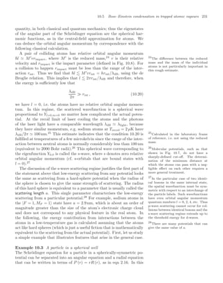
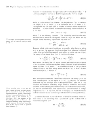
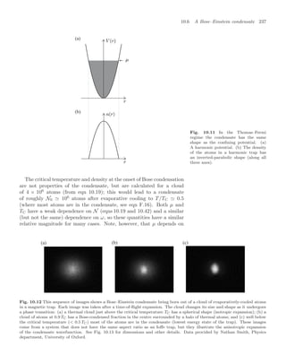
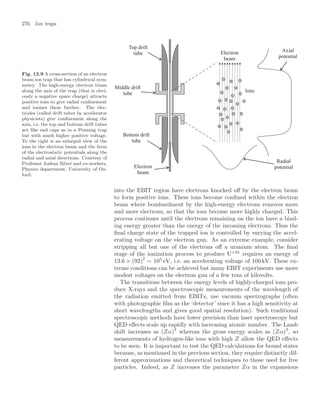
254. 10.7 Properties of Bose-condensed gases 239
To observe the condensate experimenters record an image by illumi-
nating the atoms with laser light at the resonance frequency.43
Typically, 43
Generally, absorption gives a better
signal than fluorescence but the optical
system and camera are similar in both
cases.
the experiments have an optical resolution of about 5 µm, so that the
length of the condensate can be measured directly but its width is not
precisely determined. Therefore the magnetic trap is turned off sharply
so that the atoms expand and some time later a laser beam, that passes
through the cloud of atoms onto a camera, is flashed on to record a
shadow image of the cloud. The repulsion between atoms causes the
cloud to expand rapidly after the confining potential is switched off (see
Exercise 10.6). The cigar-shaped cloud expands more rapidly in the ra-
dial direction (x and y) than along z, so that after several milliseconds
the radial size becomes bigger than that along z, i.e. the aspect ratio
inverts.44
In contrast, the uncondensed atoms behave as a classical gas 44
This expansion of the wavefunction is
predicted by including time dependence
in the nonlinear Schrödinger equation.
and expand isotropically to give a spherical cloud, since by definition the
thermal equilibrium implies the same kinetic energy in each direction.
Pictures such as Fig. 10.12 are the projection of the density distribution
onto a two-dimensional plane, and show an obvious difference in shape
between the elliptical condensate and the circular image of the thermal
atoms. This characteristic shape was one of the key pieces of evidence
for BEC in the first experiment, and it is still commonly used as a di-
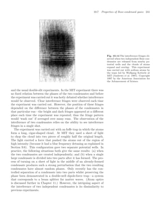
agnostic in such experiments. Figure 10.13 shows the density profile of
the cloud of atoms released from a magnetic trap for temperatures close
to the critical point, and below.
10.7 Properties of Bose-condensed gases
Two striking features of Bose-condensed systems are superfluidity and
coherence. Both relate to the microscopic description of the condensate
as N atoms sharing the same wavefunction, and for Bose-condensed
gases they can be described relatively simply from first principles (as
in this section). In contrast, the phenomena that occur in superfluid
helium are more complex and the theory of quantum fluids is outside
the scope of this book.
10.7.1 Speed of sound
To estimate the speed of sound vs by a simple dimensional argument we
assume that it depends on the three parameters µ, M and ω, so that45 45
The size of the condensate R is not
another independent parameter, see
eqn 10.40.
vs ∝ µα
Mβ
ωγ
. (10.43)
This dimensional analysis gives46 46
Comparing the dimensions of the
terms in eqn 10.43 gives
m s−1
= [kg m2
s−2
]α
kgβ
s−2γ
.
Hence α = −β = 1/2 and γ = 0.
vs
µ
M
. (10.44)
This corresponds to the actual result for a homogeneous gas (without us
needing to insert any numerical factor), and gives a fairly good approx-
imation in a trapped sample. The speed at which compression waves

255. 240 Magnetic trapping, evaporative cooling and Bose–Einstein condensation
travel in the gas has great significance for superfluidity. For motion
slower than this speed the condensate flows smoothly around obstacles
without exciting any particles out of the ground state of the quantum
gases. This type of flow does not dissipate any energy and so it is fric-
tionless and the gas is superfluid.
10.7.2 Healing length
The Thomas–Fermi approximation neglects the kinetic energy term in
the Schrödinger equation. This leads to a physically unrealistic sharp
edge at the surface of the condensate (see Fig. 10.11)—such a discon-
tinuity in the gradient would make ∇2
ψ infinite. Therefore we have
to take kinetic energy into account at the boundary. To determine the
shortest distance ξ over which the wavefunction can change we equate
the kinetic term (that contains ∇2
ψ 2
/(2Mξ2
)) to the energy scale
of the system given by the chemical potential. Atoms with energy higher
than µ leave the condensate. Using n0 = Nµ/g (from eqn 10.39) and
eqn 10.30 for g, we find that
2
2Mξ2
µ =
gn0
N
=
4π2
an0
M
. (10.45)
Hence ξ = 1/
√
8πan0, e.g. ξ = 0.3 µm for a sodium condensate with
n0 = 2 × 1014
cm−3
. Typically, ξ Rx and smoothing of the wavefunc-
tion only occurs in a thin boundary layer, and these surface effects give
only small corrections to results calculated using the Thomas–Fermi ap-
proximation. This so-called healing length also determines the size of the
vortices that form in a superfluid when the confining potential rotates
(or a fast moving object passes through it). In these little ‘whirlpools’
the wavefunction goes to zero at the centre, and ξ determines the dis-
tance over which the density rises back up to the value in the bulk of
the condensate, i.e. this healing length is the distance over which the
superfluid recovers from a sharp change.
10.7.3 The coherence of a Bose–Einstein
condensate
Figure 10.14 shows the result of a remarkable experiment carried out by
the group led by Wolfgang Ketterle at MIT. They created two separate
condensates of sodium at the same time. After the trapping potential
was turned off the repulsion between the atoms caused the two clouds to
expand and overlap with each other (as in the time-of-flight technique
used to observe Bose–Einstein condensation, see Fig. 10.12). The two
condensates interfere to give the fringes shown in the figure; there are
no atoms at certain positions where the matter waves from the two
sources interfere destructively—these atoms do not disappear, but they
are redistributed to positions in the fringe pattern where the matter
waves add constructively. Such interference is well known in optics;
however, there is a very interesting difference between this experiment

256. 10.7 Properties of Bose-condensed gases 241
Fig. 10.14 The interference fringes ob-
served when two independent Bose con-
densates are released from nearby po-
tential wells and the clouds of atoms
expand and overlap. This experiment
was carried out with sodium atoms by
the team led by Wolfgang Ketterle at
MIT (Andrews et al. 1997). Copyright
1997 by the American Association for
the Advancement of Science.
and the usual double-slit experiments. In the MIT experiment there was
no fixed relation between the phases of the two condensates and before
the experiment was carried out it was hotly debated whether interference
would be observed. Clear interference fringes were observed each time
the experiment was carried out. However, the position of these fringes
depended on the difference between the phases of the condensates in
that particular run—the bright and dark fringes appeared at a different
place each time the experiment was repeated; thus the fringe pattern
would ‘wash out’ if averaged over many runs. The observation of the
interference of two condensates relies on the ability to see interference
fringes in a single shot.
The experiment was carried out with an Ioffe trap in which the atoms
form a long, cigar-shaped cloud. At MIT they used a sheet of light
to chop the cloud into two pieces of roughly half the original length.
The light exerted a force that pushed the atoms out of the region of
high intensity (because it had a blue frequency detuning as explained in
Section 9.6). This configuration gave two separate potential wells. In
practice, the following situations both give the same results: (a) when
the two condensates are created independently; and (b) when a single
large condensate is divided into two parts after it has formed. The pro-
cess of turning on a sheet of light in the middle of an already-formed
condensate produces such a strong perturbation that the two resulting
condensates have almost random phases. Only recently has the con-
trolled separation of a condensate into two parts whilst preserving the
phase been demonstrated in a double-well dipole-force trap—a system
that corresponds to a beam splitter for matter waves. (Atom optics
is discussed further in Chapter 11.) However, the intriguing aspect of
the interference of two independent condensates is its dissimilarity to
previous experiments.

257. 242 Magnetic trapping, evaporative cooling and Bose–Einstein condensation
Fig. 10.15 Atoms coupled out of a
Bose–Einstein condensate fall down-
wards under gravity to form a well-
collimated matter-wave beam, with
analogous properties to the beam of
light from a laser. Courtesy of Nathan
Smith and William Heathcote, Physics
department, University of Oxford.
100 m
µ
10.7.4 The atom laser
The phrase ‘atom laser’ has been used to describe the coherent beam of
matter waves coupled out of a Bose–Einstein condensate (as shown in
Fig. 10.15). After forming the condensate, the radio-frequency radiation
was tuned to a frequency that drives a transition to an untrapped state
(e.g. MF = 0) for atoms at a position inside the condensate. (This comes
from the same source of radiation used for evaporative cooling.) These
atoms fall downwards under gravity to form the beam seen in the figure.
These matter waves coupled out of the condensate have a well-defined
phase and wavelength like the light from a laser.47
Many novel matter-
47
The atoms accelerate as they fall un-
der gravity so the wave propagation is
different to that of light.
wave experiments have been made possible by Bose–Einstein condensa-
tion, e.g. the observation of nonlinear processes analogous to nonlinear
optics experiments that were made possible by the high-intensity light
produced by lasers.
10.8 Conclusions
Bose–Einstein condensation in dilute alkali vapours was first observed in
1995 by groups at JILA (in Boulder, Colorado) and at MIT, using laser
cooling, magnetic trapping and evaporation. This breakthrough, and
the many subsequent new experiments that it made possible, led to the
award of the Nobel prize to Eric Cornell, Carl Wieman and Wolfgang
Ketterle in 2001 (and the Nobel prize web site has much useful informa-
tion on this subject, with links to the web sites of the research groups).
Recent BEC experiments have produced a wealth of beautiful images;
however, the objective of this chapter has not been to cover everything
but rather to explain the general principles of the underlying physics.
The two books on BEC by Pethick and Smith (2001) and Pitaevskii and
Stringari (2003) contain much more detail.

258. Exercises for Chapter 10 243
Exercises
(10.1) Magnetic trapping
An Ioffe–Pritchard trap has a radial gradient of
b
= 3 T m−1
, and the combination of Helmholtz
and pinch coils gives a field along z with B0 =
3×10−4
T and curvature b
= 300 T m−2
. Calcu-
late the oscillation frequencies of sodium atoms
in the trap.
(10.2) Loading a trap
(a) A spherical cloud of 1010
sodium atoms with
a density of around 1010
cm−3
and a tem-
perature of T = 2.4 × 10−4
K is placed in
a spherically-symmetric trapping potential.
The temperature and density of the cloud are
preserved during this loading if
1
2
Mω2
r2
=
1
2
kBT . (10.46)
Calculate the trapping frequency ω that ful-
fils this mode-matching condition, and ex-
plain what happens if the trap is too stiff or
too weak. (In a precise treatment r would be
the root-mean-square radius of a cloud with
a Gaussian density distribution.)
(b) Calculate nλ3
dB/2.6 for the trapped cloud, i.e.
the ratio of its phase-space density to that re-
quired for BEC (eqn 10.14).
(c) After loading, an adiabatic compression of
the trapped cloud changes the oscillation fre-
quencies of the atoms to ωr/2π = 250 Hz
and ωz/2π = 16 Hz. The phase-space density
does not change during adiabatic processes,
i.e. nλ3
dB is constant. Show that this implies
that T V 2/3
is constant. Calculate the tem-
perature and density of the cloud after com-
pression.48
(10.3) Magnetic trapping
(a) Sketch the energy of the hyperfine levels
of the 3s 2
S1/2 ground level of sodium as
a function of the applied magnetic field
strength. (The hyperfine-structure constant
of this level is A3s = 886 MHz and sodium
has nuclear spin I = 3/2.)
(b) What is meant by a ‘weak’ field in the con-
text of hyperfine structure?
(c) Show that for a weak magnetic field the
states in both hyperfine levels have a split-
ting of 7 GHz T−1
.
(d) Explain why the potential energy of an atom
in a magnetic trap is proportional to the
magnetic flux density |B|.
A magnetic trap has a field that can be ap-
proximated by
B = b
(xêx − yêy)
in the region where r = (x2
+ y2
)1/2
⩽
10 mm, and B = 0 outside this radius. The
field gradient b
= 1.5 T m−1
and the z-axis
of the trap is horizontal.
(e) Calculate the ratio of the magnetic force on
the atoms compared to that of gravity.
(f) Estimate the maximum temperature of
atoms that can be trapped in the (i) upper
and (ii) lower hyperfine levels. State the MF
quantum number of the atoms in each case.
(Assume that the confinement of atoms along
the z-axis is not the limiting factor.)
(g) For the clouds of trapped atoms in both (i)
and (ii) of part (f), describe the effect of ap-
plying radio-frequency radiation with a fre-
quency of 70 MHz.
48The relation between temperature and volume can also be derived from thermodynamics: TV γ−1 is constant for an adia-
batic change in an ideal gas and a monatomic gas has a ratio of heat capacities γ = CP/CV = 5/3. Actually, the phase-space
density only remains constant if the potential has the same shape throughout the adiabatic change. In the case of an Ioffe trap,
the radial potential may change from harmonic to linear (see Example 10.2), giving a small increase in the phase-space density.
This effect arises because the population of the energy levels stays the same but the distribution of the levels changes—the
energy levels of a harmonic potential are equally spaced (ω apart), whereas in a linear potential the intervals between levels
decrease with increasing energy.

259. 244 Magnetic trapping, evaporative cooling and Bose–Einstein condensation
(10.4) Evaporative cooling
A cloud of atoms has a Boltzmann energy distri-
bution N (E) = Ae−βE
, where 1/β = kBT and
the normalisation constant A is found from
Ntotal = A
∞
0
e−βE
dE =
A
β
.
The cloud has a total energy given by
Etotal = A
∞
0
Ee−βE
dE =
A
β2
= NtotalkBT .
Hence each atom has a mean energy E = kBT. In
an evaporative cooling step all atoms with energy
greater than escape.
(a) Calculate the fraction of atoms lost
∆N/Ntotal.
(b) Calculate the fractional change in the mean
energy per atom.
(c) Evaluate your expressions for cuts with β =
3 and 6. Compare the ratio of energy lost
and the number of atoms removed in the two
cases and comment on the implications for
evaporative cooling.
(d) The collision rate between atoms in the cloud
is Rcoll = nvσ. Assuming that the collision
cross-section σ is independent of the energy,
show that Rcoll ∝ Ntotal/Etotal in a harmonic
trapping potential. Show that the collision
rate increases during evaporation in such a
potential.
(10.5) The properties at the phase transition
A cloud of 106
rubidium atoms is confined in
a harmonic trap with oscillation frequencies of
ωz/2π = 16 Hz and ωr/2π = 250 Hz (and axial
symmetry). Calculate the critical temperature
TC and estimate the density of the cloud at the
phase transition.
(10.6) Properties of a Bose condensate
The properties of a Bose condensate were calcu-
lated in the text using the Thomas–Fermi approx-
imation, which gives accurate results for large
condensates. This exercise shows that minimis-
ing the energy in eqn 10.33 (a variational calcula-
tion) to find the equilibrium size leads to similar
results.
In a spherically-symmetric trapping potential,
rubidium atoms (M = 87 a.m.u.) have an os-
cillation frequency of ω/2π = 100 Hz and hence
aho = 1 µm. The atoms have a scattering length
of a = 5 nm. Calculate the following for a con-
densate with N0 = 106
atoms.
(a) Show that the repulsive interactions give a
much greater contribution to the total energy
than the kinetic term.
(b) Use eqn 10.33 to find an expression for the
equilibrium size r and evaluate it.
(c) What is the density of the condensate?
(d) Show that the contribution to the energy
from the repulsive interactions represents
two-fifths of the total.
(e) Find an expression for the energy E (in terms
of ω). (Note that this expression should
have the same dependence on the various pa-
rameters as in eqn 10.42, but with a different
numerical factor.) Evaluate E/kB.
(f) When the trapping potential is switched off
suddenly the potential energy goes to zero
and the repulsive interaction between the
atoms causes the condensate to expand. Af-
ter a few milliseconds almost all this energy
(from the repulsive interactions) is converted
into kinetic energy. Estimate the velocity
at which the atoms fly outwards and the
size of the condensate 30 ms after the trap
is switched off.49
Comment. These estimates of the important
physical parameters show that, although inter-
actions have little influence on the phase transi-
tion (Bose–Einstein condensation occurs because
of quantum statistics and is completely different
to the ‘ordinary’ condensation of a vapour into
a liquid caused by molecular interactions, e.g.
steam into water), the properties of the conden-
sate itself do depend on the interactions between
atoms, e.g. the energy of the condensate is much
larger than the zero-point energy of the ground
state of the quantum harmonic oscillator.
(10.7) The chemical potential and mean energy per
particle
(a) Show that eqn 10.42 follows from the preced-
ing equations in Section 10.6.
49The small size of Bose condensates makes them difficult to view directly, although this has been done in certain experiments.
Generally, the condensate is released from the trap and allowed to expand before an image (e.g. Fig. 10.12).

260. Exercises for Chapter 10 245
(b) In thermodynamics the chemical potential is
the energy required to remove a particle from
the system µ = ∂E/∂N, where E is the total
energy of the system. Show that E = 5
7
Nµ.
(10.8) Expansion of a non-interacting condensate
Although experiments are not carried out with
a non-interacting gas it is instructive to consider
what happens when a = 0. In this case the con-
densate has the same size as the ground state
of a quantum harmonic oscillator (for any N0)
and the initial momentum along each direction
can be estimated from the uncertainty principle.
For atoms of the same mass as sodium (but with
a = 0) released from a trap with a radial os-
cillation frequency of 250 Hz and a frequency of
16 Hz for axial motion, estimate roughly the time
of flight at which the cloud is spherical.
(10.9) Excitations of a Bose condensate
The vibrational modes of a condensate can be
viewed as compression waves that form a stand-
ing wave within the condensate; hence these
modes have frequencies of the order of the speed
of sound divided by the size of the condensate
vs/R. Show that this collective motion of the
condensate occurs at a comparable frequency to
the oscillation of individual atoms in the mag-
netic trap.
(10.10) Derivation of the speed of sound
The time-dependent Schrödinger equation for the
wavefunction of an atom in a Bose–Einstein con-
densate in a uniform potential is
i
dψ
dt
= −
2
2M
∇2
ψ + g |ψ|2
ψ ,
where, for simplicity, the potential has been taken
as zero (V = 0). The wavefunction ψ = ψ0e−iµt/
satisfies this equation with a chemical potential
µ = g |ψ0|2
.
The trial wavefunction with small fluctuations
can be written as
ψ =
5
ψ0 + uei(kx−ωt)
+ v∗
e−i(kx−ωt)
6
e−iµt/
= ψ0e−iµt/
+ δψ (t) ,
where the amplitudes |u| and |v| are small com-
pared to |ψ0|.
(a) Show that substituting this function into the
Schrödinger equation and making suitable
approximations leads to the same zeroth-
order approximation for the chemical poten-
tial given above and
i
d
dt
(δψ (t))
=
2
k2
2M
δψ (t) + g |ψ0|2
2δψ (t) + gψ2
0δψ∗
(t) .
(10.47)
(b) Show that equating terms with the same time
dependence leads to two coupled equations
for u and v that, in matrix form, are
k + 2g |ψ0|2
− µ gψ2
0
g(ψ∗
0 )2
k + 2g |ψ0|2
− µ
u
v
= ω
u
−v
,
where k = 2
k2
/2M.
(c) Hence show that u and v are solutions of the
matrix equation
k + µ − ω gψ2
0
g(ψ∗
0 )2
k + µ + ω
u
v
= 0 .
From the determinant of this matrix, find
the relation between the angular frequency of
the small oscillations ω and the magnitude of
their wavevector k (the dispersion relation).
Show that for low energies this gives the same
expression for the speed of sound ω/k found
in Section 10.7.1.50
(10.11) Attractive interactions
In certain hyperfine states, the scattering length
a of alkali metal atoms changes with the applied
magnetic field and this feature has been used to
perform experiments in which the atoms have at-
tractive interactions a 0.
Show that eqn 10.33 can be written in the form
4
3
E
ω
= x−2
+ x2
+ Gx−3
.
By plotting graphs for various values of the pa-
rameter G between 0 and −1, estimate the lowest
value of G for which there exists a minimum in
the energy as a function of x. For an atomic
species with a scattering length of a = −5 nm
in a trap where aho = 2 µm, estimate the max-
imum number of atoms that a Bose condensate
can contain without collapsing.
50After problem devised by Professor Keith Burnett, Physics graduate class, University of Oxford.

261. Atom interferometry
11
11.1 Young’s double-slit
experiment 247
11.2 A diffraction grating for
atoms 249
11.3 The three-grating
interferometer 251
11.4 Measurement of rotation 251
11.5 The diffraction of atoms
by light 253
11.6 Conclusions 257
Further reading 258
Exercises 258
The possibility of interferometry with atoms follows directly from wave–
particle duality. The wave-like propagation of particles, such as atoms,
means that they undergo interference and diffraction in an analogous
way to light. This chapter explains how such matter waves have been
used in interferometers that measure rotation and gravitational acceler-
ation to a precision comparable with the best optical instruments. As
in many important developments in physics, atom interferometry relies
on simple principles—the first part of this chapter uses only elementary
optics and the de Broglie relation
λdB =
h
p
(11.1)
for the wavelength of the matter wave associated with a particle of mo-
mentum p = Mv. This relation between wavelength and momentum
also applies to light waves and the momentum of photons, but here we
shall use λdB exclusively for matter waves and λ, without a subscript,
for the wavelength of light.
A sodium atom with velocity v = 1000 m s−1
(typical of a thermal
beam) has λdB = 2 × 10−11
m—about 1/30 000 times the wavelength of
visible light, and comparable to that of X-ray radiation. Gratings with
lines sufficiently close together to diffract such short wavelengths can
now be made by nano-fabrication, i.e. techniques for making structures
on scales smaller than 1 µm.1
Neutrons also have short de Broglie wave-
1
It might seem advantageous to use
laser-cooled atoms with larger λdB, but
we shall see that this is not true.
lengths but, unlike atoms, they pass through crystals and diffract from
the closely-spaced planes of atoms. Electrons also diffract from crystals
and their wave properties were observed long ago by Davisson and Ger-
mer in their classic experimental confirmation of wave–particle duality
in quantum physics. This previous work with neutrons and electrons is
mentioned here simply to show that matter-wave interferometry has a
long history, and both neutron and electron diffraction are now highly-
developed techniques used in condensed matter physics (Blundell 2001).
The more recent matter-wave experiments with atoms described in this
chapter should not be regarded as tests of already well-known quantum
behaviour; rather their importance lies in their ability to make more
precise measurements than other techniques in certain applications.
Consideration of the familiar Young’s double-slit experiment provides
a good introduction to the basic ideas of matter-wave experiments with
atoms and gives a feeling for the size of the physical parameters. We
shall then extend the treatment to a diffraction grating (multiple slits)
and the design of an interferometer that measures the rate of rotation by

262. 11.1 Young’s double-slit experiment 247
the Sagnac effect. These matter-wave experiments operate on the same
principles as similar experiments with light because the atoms remain in
the ground state and propagate as simple waves. It will be assumed that
the reader understands the standard treatment of Fraunhofer diffraction
in optics (Brooker 2003) and key results will be quoted here rather than
derived. After the discussion of the work with nano-fabricated slits and
gratings, we shall look at the use of laser light to manipulate the atom’s
momentum using methods closely related to laser cooling. These laser
techniques make use of the atom’s internal energy levels—something
that is not possible for electrons or neutrons.
11.1 Young’s double-slit experiment
Young originally carried out his double-slit experiment to test the wave
nature of light and his simple arrangement still finds practical use in
measurements of the coherence of light.2
Figure 11.1 shows a typical 2
The double slits also form the basis
of many theoretical discussions of fun-
damental issues in quantum mechanics,
such as why we cannot know which slit
the photon went through and still ob-
serve interference.
experimental layout. Waves propagate from the source slit S through
the two slits, Σ1 and Σ2, to a point P in the detection plane.3
The
3
Young’s fringes are not localised on
this plane but can be seen throughout
the far-field region.
amplitude of the light at any point on the detection plane equals the
sum of the electric field amplitudes that arrive at that point via slits
Σ1 and Σ2. In any interference or diffraction calculation the resultant
amplitude at the final point is determined by summing the contributions
from all possible paths taking account of the phase. For the double slits
Detector
(a)
(b)
Fig. 11.1 (a) The apparatus for observing interference from double slits. The light diffracted by the source slit propagates
through the two slits Σ1 and Σ2 and onto the plane P. The interference fringes can be seen with the eye (with the aid of
a magnifying eyepiece if necessary), but to further the analogy with atom optics experiments the apparatus is drawn with a
detector such as a photodiode or photomultiplier. A narrow slit in front of the detector gives good spatial resolution; this slit
and the detector scan across the fringes, as indicated. The light comes from a lamp, or laser; in a matter-wave experiment an
atomic oven creates a beam of atoms collimated by the source slit (as shown in Fig. 11.2). (b) The difference in the distance
from Σ1 to P and from Σ2 to P is d sin θ, where d is the slit separation. The angle θ and the distance X in the detection plane
are related by X = L tan θ. The transverse distances are drawn greatly exaggerated for clarity; for the typical conditions given
in the text the fringes have an angular separation of 2 × 10−3 rad.

263. 248 Atom interferometry
we define l1 as the distance from S to P via Σ1, and similarly l2 for the
path through slit Σ2, as shown by the dotted lines in Fig. 11.1(b).4
Slits
4
l1 = SΣ1 + Σ1P and l2 = SΣ2 + Σ2P.
of the same size contribute equally to the total amplitude at a point on
the plane P:
EP ∝ E0
$
e−i2π 1/λ
+ e−i2π 2/λ
. (11.2)
The intensity is proportional to the square of this amplitude, I ∝ |E|2
,
so that
I = I0 cos2
φ
2
. (11.3)
Here φ = 2π(2 − 1)/λ is the phase difference between the two arms
and I0 is the maximum intensity. Bright fringes occur at positions in
the detection plane where the contributions from the two paths inter-
fere constructively; these correspond to φ = n2π, with n an integer, or
equivalently
2 − 1 = nλ . (11.4)
To find the spacing of the fringes in the plane of observation we define
the coordinate X measured perpendicular to the long axis of the slits
in the plane P. In terms of the small angle defined in Fig. 11.1(b) this
becomes
X = L tan θ . (11.5)
A similar small angle approximation allows us to express the path length
difference in Fig. 11.1(b) as
2 − 1 = ∆l + d sin θ . (11.6)
Here ∆l = SΣ1 − SΣ2 is the path difference before the slits.5
The path
5
Elementary treatments often assume
that the slits are equidistant from the
source (∆l = 0) so that the phase of the
wave is the same at each slit (equivalent
to having a plane wavefront before the
slits). This assumption simplifies the
algebra but it is not a necessary con-
dition for Fraunhofer diffraction with
light, or with matter waves. (A more
detailed description of the assumptions
such as L d can be found in text-
books on optics, e.g. Brooker (2003).)
length difference from the two slits of separation d to P is d sin θ. The
last three equations give the spacing of the fringes as
∆X =
L λ
d
. (11.7)
For an experiment with visible light of wavelength λ = 6 × 10−7
m, slits
of separation d = 3 × 10−4
m and L = 1 m, the fringes have a spacing
of ∆X = 2 mm and can be clearly seen by eye. The treatment so far
assumes a small source slit at S that acts like a point source to illuminate
the double slits coherently. The condition for this is that the double slits
fall within the angular spread of the light diffracted from the source slit
(Brooker 2003). The diffraction from a slit of width wS has an angular
spread θdiff λ/wS. Therefore coherent illumination of two slits at a
distance L
from this source slit requires L
θdiff ⩾ d, or
wS ⩽
λL
d
. (11.8)
For L
= 0.1 m and the values of λ and d used previously, we find
wS ⩽ 2 × 10−4
m. Such slits are made by standard techniques and we
know that Young’s experiment with light is relatively straightforward to

264. 11.2 A diffraction grating for atoms 249
carry out in the laboratory. Experiments with short-wavelength matter
waves require the smallest available structures with slits on the scale of
100 nm.
A double-slit experiment was carried out with a beam of helium atoms
in the metastable 1s2s 3
S1 level that lies 20 eV above the ground state
(Carnal and Mlynek 1991). This matter-wave experiment had the same
layout as that shown in Fig. 11.1, although with atoms the interfer-
ometer has to be set up inside a vacuum chamber. Exercise 11.2 goes
through the application of the equations given in this section to the cal-
culation of the slit widths required to observe interference fringes with
He∗
. Metastable helium is very suitable for this experiment, firstly be-
cause it has a fairly long λdB and secondly when metastable atoms hit
a surface they release sufficient energy to eject electrons; counting these
charged particles allows the arrival of individual atoms to be detected
with high efficiency. Further discussion of double-slit experiments can be
found in the quantum mechanics book by Rae (1992); he uses a neutron
interference experiment as an example of wave–particle duality.
11.2 A diffraction grating for atoms
Figure 11.2 shows an apparatus with a highly-collimated atom beam
of sodium incident upon a transmission grating. The experimenters
used a remarkable grating with slits only 50 nm wide, spaced 100 nm
apart—equal widths of the bars and the gaps between them. Etching
these very thin bars and their delicate support structure represents the
state of the art in nano-fabrication. Figure 11.2(b) shows the diffraction
pattern obtained with a mixture of sodium atoms and molecules, and
Fig. 11.2(c) shows the diffraction of a beam of sodium molecules. The
diffraction peaks of Na2 have about half the spacing of those for the Na
atoms, as expected from the de Broglie relation for particles of twice the
mass (for similar velocities).
Researchers recently exploited this property of these special gratings
to make the first experimental observation of the very weakly-bound
state of two helium atoms (Schöllkopf and Toennies 1994). Other meth-
ods of detection dissociate the very tenuously-bound He2 molecule. The
gratings work well with helium and atomic beams of inert gases, since
they do not clog the slits in the same way as sodium. However, despite
the practical difficulties of working with these very fragile structures,
a recent experiment used a grating to diffract C60 molecules—so-called
Buckyballs (Arndt et al. 1999, Nairz et al. 2003). This demonstration
of the wave-like nature of such massive particles prompts the following
question: ‘What is the largest object for which such quantum inter-
ference can be observed?’6
This question relates to Schrödinger’s well- 6
This means quantum effects in the
motion, or external degrees of freedom,
and not quantisation of the internal en-
ergy levels.
known example of a cat that may be in a superposition of two states
(‘alive’ and ‘dead’). To observe interference an object must exist in
a superposition of the two states: |1 in which it goes through slit Σ1
and |2 the state where it goes through slit Σ2. Nothing within standard

265. 250 Atom interferometry
(c)
(b)
(a)
Counts/second
Detector position ( m)
−1000 −500 500 1000
0
104
103
104
103
Detector
Grating
Supersonic beam
of atoms and molecules
Source
Carrier
gas
Detector position ( m)
−1000 −500 500 1000
0
Fig. 11.2 (a) Diffraction of a collimated atomic beam by a grating. To observe the diffraction of matter waves from the grating
the source slit must be sufficiently narrow to make the matter waves coherent across several of the slits in the grating. This
is the same requirement as described in the previous section for Young’s double slits, and Exercise 11.1 looks at the relation
of the pattern with multiple slits to that observed with just two slits. For the grating there is an additional requirement that
the angular spread of the incident beam must be less than the angle between the diffracted orders, otherwise they cannot be
distinguished. In this apparatus the slit widths were about 20 µm, the slits in the nano-fabricated grating had a spacing of
100 nm and all the distances LC, L and L were about 1 m. (b) The diffraction of a collimated beam of sodium atoms and
molecules by the grating. (c) The diffraction pattern for a beam that contains only Na2 molecules (this pattern is also shown
as a dotted curve in (b)). The peaks for the molecules have half the spacing of those for the atoms as expected for twice the
mass—the atoms and molecules have almost the same velocity in the supersonic flow because they are both carried along in a
stream of krypton gas that flows through the heated oven containing sodium metal. This carrier gas gives a supersonic beam
with a much lower velocity spread ∆v/v 0.03 than would be obtained from an effusive source of thermal atoms. The sodium
atoms were removed from the beam by the resonant radiation pressure from a laser beam (not shown) perpendicular to the
supersonic beam—scattering three or more photons was sufficient to deflect atoms out of the beam. From Chapman et al.
(1995). Copyright 1995 by the American Physical Society.

266. 11.4 Measurement of rotation 251
quantum mechanics tells us that we cannot put something as large as
a cat into a quantum superposition, if it is completely isolated from
external perturbations. However, the heaviest object that can be used in
a practical double-slit experiment in the foreseeable future is far lighter
than a cat, but considerably heavier than what has been achieved so far.
Continued work on matter-wave interference of larger and larger objects
will be of great interest since it probes the boundary between quantum
and classical physics.
11.3 The three-grating interferometer
Figure 11.3 shows an arrangement of three diffraction gratings a distance
L apart. A highly-collimated beam of sodium atoms propagates through
this three-grating interferometer onto a detector for atoms.7
Diffraction 7
The detector for sodium has a hot
wire, heated by a current flowing
through it, that runs parallel to the
slits. The sodium atoms ionize when
they hit the hot surface of the wire and
the ejected electrons create a measur-
able current.
at the first grating G1 splits the beam—only the zeroth- and first-order
diffraction orders (0 and ±1 orders) have been drawn for simplicity. The
second grating G2 gives diffraction through the same angles as G1, so
that some of the paths meet up at the plane of the third grating G3,
e.g. the 0 and +1 orders from G1 are both diffracted by G2 to form the
parallelogram ABPC, as shown in Fig. 11.3(a). The detector records the
flux of atoms along one of the possible output directions coming from
P. This arrangement closely resembles a Mach–Zehnder interferometer
for light, with a smaller angle between the two arms because of the
achievable grating spacing. For two-beam interference the signal has
the same form as eqn 11.3. In these interferometers the sum of the
fluxes of the atoms, or light, in the two possible output directions equals
a constant, i.e. when a certain phase difference between the arms of the
interferometer gives destructive interference at the detector then the flux
in the other output direction has a maximum.
11.4 Measurement of rotation
The Mach–Zehnder interferometer for matter waves shown in Fig. 11.3
measures rotation precisely, as explained in this section.8
To calculate 8
For light a different configuration
called a Sagnac interferometer is gen-
erally used to measure rotation but the
principles are similar.
the phase shift caused by rotation in a simple way we represent the
interferometer as a circular loop of radius R, as in Fig. 11.4. The wave
travelling at speed v from the point S takes a time t = πR/v to propagate
around either arm of the interferometer to the point P diametrically
opposite S. During this time the system rotates through an angle Ωt,
where Ω is the angular frequency of rotation about an axis perpendicular
to the plane of the interferometer. Thus the wave going one way round
the loop has to travel ∆l = 2ΩRt further than the wave in the other arm
of the interferometer. This corresponds to ∆l/λdB extra wavelengths,
or a phase shift of
∆φ =
2π
λdB
× 2ΩR ×
πR
v
. (11.9)

267. 252 Atom interferometry
S
Detector
M1
M2
BS1
BS2
(a)
(b)
(c)
G1
Collimated beam
of atoms
G2
Order of
diffraction
Detector
G3
Detector
Fig. 11.3 (a) An interferometer formed by three diffraction gratings spaced by a distance L along the atomic beam. A
collimated beam of atoms is produced, as shown in Fig. 11.2. Waves diffracted at the first grating G1 split again at G2, so
that some of the paths meet at G3. Only the 0 and ±1 diffraction orders are shown and to further simplify the diagram some
of the possible paths between G2 and G3 have not been drawn completely. Contributions to the amplitude at P arrive from
A, via either B or C. The detector must be sufficiently far from G3 that it picks up only one of two possible output directions.
(The parallelogram ABPC is just one of many closed loops formed by the three gratings; some others are indicated by dotted
lines. With the detector at the position shown, the three gratings act as a Mach–Zehnder interferometer, as shown in (b). The
diffraction gratings behave both as beam splitters and as deflectors (mirrors) for the matter waves (for small angles). (c) A
Mach–Zehnder interferometer for light—the optical system equivalent to the three-grating interferometer. The incident wave
hits beam splitter BS1 and the reflected and transmitted amplitudes reflect off mirrors M1 and M2, respectively, so that their
paths meet again at BS2. Interference between the two paths leads to a detected intensity ID = 1
2
I0{1 + cos(φ + ∆φ)} (cf.
eqn 11.3). The phase φ that arises from path length differences and phase shifts on reflection at the mirrors is assumed to be
fixed and ∆φ represents the extra phase that is measured; e.g. for an interferometer that rotates at angular frequency Ω about
an axis perpendicular to the plane of the instrument ∆φ ∝ Ω, so the instrument measures rotation, as shown in Section 11.4.
The loop has area A = πR2
, so that
∆φ =
4π
λdBv
× ΩA . (11.10)
A more rigorous derivation, by integration around a closed path, shows
that this equation applies for an arbitrary shape, e.g. the square interfer-
ometer of Fig. 11.3(c). Comparison of this phase shift for matter waves
of velocity v with that for light ∆φlight, for an interferometer of the same

268. 11.5 The diffraction of atoms by light 253
S S
P P
(a) (b)
Fig. 11.4 (a) A simplified diagram
of an interferometer where the waves
propagate from S to P. (b) Rotation at
angular frequency Ω about an axis per-
pendicular to the plane of the interfer-
ometer makes one path Ωt longer and
the other shorter by the same amount,
where t is the time taken for a wave to
travel from S to P. This leads to the
phase shift in eqn 11.10.
area A, shows that
∆φ =
λc
λdBv
× ∆φlight =
Mc2
ω
× ∆φlight . (11.11)
The ratio equals the rest mass of the atom divided by the energy of each
photon and has a value of ∆φ/∆φlight ∼ 1010
for sodium atoms and
visible light. This huge ratio suggests that matter-wave interferometers
have a great advantage, but at the present time they only achieve com-
parable results to conventional interferometers with light. Conventional
interferometers with light make up the ground by:
(a) having much larger areas, i.e. a distance between the arms of metres
instead of a fraction of a millimetre achieved for matter waves;
(b) the light goes around the loop many times;9 9
Laser gyros use high-reflectivity mir-
rors or optical fibres.
(c) lasers give a much higher flux than the flux of atoms in a typical
atomic beam. For example, in the scheme shown in Fig. 11.2 only
a small fraction of the atoms emitted from the source end up in
the highly-collimated atomic beam; as a source of matter waves the
atomic oven is analogous to an incandescent tungsten light bulb
rather than a laser.10
10
The atom interferometer based on
Raman transitions (described in Sec-
tion 11.5.1) does not require such a
highly-collimated atomic beam, and
that technique has achieved precise
measurements of rotation.
11.5 The diffraction of atoms by light
A standing wave of light diffracts matter waves, as illustrated in Fig. 11.5.
This corresponds to a role reversal as compared to optics in which mat-
ter, in the form of a conventional grating, diffracts light. This section
explains how this light field created simply by the retro-reflection of
a laser beam from a mirror is used in atom optics. The interaction
of atoms with a standing wave leads to a periodic modulation of the
atomic energy levels by an amount proportional to the intensity of the
light, as explained in Section 9.6.11
The light shift of the atomic energy
11
The laser has a frequency ω suffi-
ciently far from the atom’s transition
frequency ω0 that spontaneous emis-
sion has a negligible effect, yet close
enough for the atoms to have a signifi-
cant interaction with the light.
levels in the standing wave introduces a phase modulation of the matter
waves. An atomic wavepacket ψ(x, z, t) becomes ψ(x, z, t) ei∆φ(x)
im-
mediately after passing through the standing wave; it is assumed that

269. 254 Atom interferometry
Fig. 11.5 The diffraction of atoms by
a standing wave light field. The an-
gle of the first order of diffraction θ
is related to the grating period d by
d sin θ = λdB. For the standing wave
d = λ/2, so sin θ = 2λdB/λ. This dif-
fraction can be regarded as a scattering
process where an atom of momentum p
receives an impulse that gives it trans-
verse momentum ∆p and deflects it by
an angle θ given by tan θ = ∆p/p.
Standing
wave
Matter
waves
Mirror
ψ(x, z, t) changes smoothly over a length scale much greater than λ/2.
This phase modulation has a spatial period of λ/2, where λ is the wave-
length of the light not the matter waves. The matter waves accumulate
an additional phase ∆φ(x) = φ0 cos2
(2πx/λ) from the light shift. This
phase grating diffracts the matter waves at angles determined by
d sin θ = nλdB , (11.12)
where d = λ/2, n is an integer and λdB gives the matter wavelength.
Gratings with the same spacing d diffract waves by the same angles θ
whether they work by phase or amplitude modulation of the incident
wave,12
although not with the same relative intensities in different or-
12
This is obvious from a treatment
of diffraction by Fourier transforms
(Brooker 2003).
ders. Thus there is no fundamental difference between nano-fabricated
absorption gratings and the use of standing waves. Interferometers that
use three standing waves in the same arrangement as in Fig. 11.3 have
similar properties to an instrument with three gratings etched from solid
material. The mirrors that retro-reflect the light to form the stand-
ing waves must be mounted rigidly so that vibrations do not wash out
the interference fringes (similarly, the nano-fabricated gratings must be
held very stable). Standing waves of visible light give diffraction angles
about three times less than those from the best nano-fabricated gratings;
however, such gratings transmit all the atoms, whereas nano-fabricated
gratings transmit much less than the 50% that might be expected for
bars that have a width equal to the gaps between them—the very thin
bars require an elaborate support structure of cross-bars that reduces
the open area. Also, material gratings eventually get clogged up when
used with alkali metals.
The diffraction of the matter waves by a standing wave has an alter-
native physical interpretation in terms of the scattering of light. The
diffraction condition in eqn 11.12 can be written as tan θ nG/p (tak-
ing tan θ sin θ for small angles), where p is the longitudinal momentum
of the atoms, G = 4π/λ is the characteristic wavevector of a structure
with spacing λ/2 (i.e. the grating) and G = 2h/λ equals the momentum
of two photons. Thus, in the diffraction from the standing wave, atoms

270. 11.5 The diffraction of atoms by light 255
receive a transverse kick from 2n photons, as illustrated in Fig. 11.5, e.g.
first order arises from absorption from one of the counter-propagating
beams and stimulated emission into the other beam. This coherent
process, with no spontaneous emission, has some similarities with the
Raman transition shown in Fig. 11.6.13
13
Scattering in a standing wave
changes the atomic momentum (ex-
ternal state) but not the internal
state.
11.5.1 Interferometry with Raman transitions
The description of the diffraction of two-level atoms by a standing wave,
in the previous section, as a coherent scattering process that imparts
twice the photon momentum 2h/λ, or multiples thereof, to the atom
has links with the very powerful method for manipulating the atom’s
momentum by Raman transitions shown in Fig. 11.6. Two laser beams
at frequencies ωL1 and ωL2 drive a coherent Raman transition between
states |1 and |2 when
(ωL1 − ωL2) = E2 − E1 . (11.13)
No population goes into the intermediate state |i in this coherent transi-
tion because neither of the two beams excites a single-photon transition
(see Appendix E). The Raman transition couples states |1 and |2 and
drives Rabi oscillations between them, e.g. when the atom starts in either
|1 or |2 , a π/2-pulse creates a superposition of |1 and |2 with equal
amplitudes. Raman laser beams propagating in opposite directions (as
in Fig. 11.6) change the atom’s momentum during the transition.14
The 14
Raman laser beams travelling in the
same direction have the same effect as
direct coupling between |1 and |2 by
microwaves.
absorption of a photon of wavevector k1 and the stimulated emission of
one in the opposite direction k2 −k1 gives the atom two recoil kicks in
the same direction. This process couples the state |1, p to |2, p + 2k .
The bra(c)ket notation denotes the |internal state, momentum of the
atoms. The Raman resonance condition in eqn 11.13 depends sensitively
on the atom’s velocity v for counter-propagating beams and this provides
the basis for the Raman cooling of atoms (Section 9.8). For interferome-
try this velocity selectivity is a complicating factor and we shall assume
that the Raman pulses are sufficiently short15
to drive transitions over 15
According to the condition in
eqn 9.58.
the whole range of velocity components along the laser beam.
Figure 11.7 shows a complete Raman interferometer where the atoms
start in |1, p and travel through three Raman interaction regions. In
Fig. 11.6 A Raman transition with
two laser beams of frequencies ωL1 and
ωL2 that propagate in opposite direc-
tions. Equation 11.13 gives the res-
onance condition, ignoring the effects
of the atom’s motion (Doppler shift).
The Raman process couples |1, p and
|2, p + 2k so that an atom in a Ra-
man interferometer has a wavefunction
of the form ψ = A|1, p + B|2, p + 2k
(usually with either B = 0 or A = 0
initially).

271. 256 Atom interferometry
Detector
Probe
beam
Lens
Key:
Fig. 11.7 An interferometer formed by Raman transitions. As atoms traverse the three interaction regions they experience a
π/2–π–π/2 sequence of Raman pulses that split, deflect and recombine the atomic wavepackets. Each interaction region has two
counter-propagating beams at frequencies ωL1 and ωL2, as in Fig. 11.6. In this Mach–Zehnder interferometer the eigenstates
with transverse momentum p and p + 2k are associated with the different internal atomic states |1 and |2, respectively;
as indicated at the bottom of the figure, |1 is associated with p 0 (horizontal line) and |2 with p 2k (slanted line).
Therefore at the output it is only necessary to measure the internal state of the atoms, e.g. by exciting a transition from |2 and
detecting the fluorescence, rather than allowing beams with different momenta to become spatially separated, as in Fig. 11.3.
(The separation of the paths has been exaggerated for clarity.)
the first interaction the atom experiences a π/2-pulse that puts it into
the superposition
|ψ =
|1, p + eiφ1
|2, p + 2k
. (11.14)
The phase factor depends on the relative phase of the two laser beams.16
16
This phase, and the other similar
phases that arise at each interaction,
lead to an offset in the final output
which is not important. But these
phases must remain constant in time,
otherwise the interference ‘washes out’.
These two states separate, as shown in Fig. 11.7, and this first region cor-
responds to a beam splitter for matter waves. After a free-flight through
a distance L the atom enters the middle interaction region where it un-
dergoes a π-pulse that acts on both arms of the interferometer to swap
the states |1, p ↔ |2, p + 2k . (In this apparatus the transit time for
the atom to pass through the laser beams determines the duration of
the Raman interaction.) The paths come back together after a further
distance L and the final π/2-pulse acts as the beam splitter that mixes
the wavepackets to give interference. The complete π/2–π–π/2 sequence
gives a Mach–Zehnder interferometer. A comparison of Figs 11.3 and
11.7 shows that the Raman scheme resembles the Mach–Zehnder inter-
ferometer more closely than the three-grating device; the Raman scheme
does not direct any amplitude in unwanted directions and the middle in-
teraction region in the Raman interferometer acts just like a mirror to
change the direction (transverse momentum) of both paths through a
small angle.17
17
In a three-grating interferometer only
a fraction of the amplitude goes in the
required direction. Note, however, that
the simple treatment of standing waves
assumed the ‘thin’ grating approxima-
tion, but often the interaction between
the matter waves and light takes place
over a sufficiently long distance that
Bragg diffraction occurs (as in crys-
tals).
A Raman pulse and standing light wave give the same opening an-
gle between the arms for a given wavelength of laser light and both

272. 11.6 Conclusions 257
schemes use light whose frequency is detuned from the atomic transition
to avoid spontaneous emission. A crucial difference between these meth-
ods arises in the detection. The three-grating apparatus, with standing
waves or nano-fabricated structures, distinguishes the two outputs by
their different directions. Therefore the three-grating devices require a
highly-collimated atomic beam at the input whose angular divergence is
less than the angle between the two output directions θdiff. The output
channels of the Raman scheme are the two different states |1, p and
|2, p + 2k , as shown in Fig. 11.7; thus experiments only need to de-
termine the final state of the atom, e.g. using a laser beam that excites
a transition from |2 to another state that gives fluorescence for atoms
in state |2 but not for those in |1 .18
This means that Raman inter-
18
As in the atomic fountain described
in Section 9.9.
ferometers use more of the atoms from a given source because they do
not need to have tight collimation.19
Although the flux of atoms does 19
The creation of the two Raman
beams with a well-defined frequency
difference, and other technical details,
are described in Section 9.8.
not affect the size of the phase shift given by eqn 11.10, the strength
of the measured signal determines how precisely that phase shift can be
measured, i.e. the interferometer measures a smaller fraction of a fringe
if the signal-to-noise ratio is higher.20
Thus the type of Raman inter-
20
This argument assumes that it is
purely statistical fluctuations (noise)
that limit the precision, not systematic
shifts.
ferometer shown in Fig. 11.7 measures rotation more precisely than a
three-grating device.
11.6 Conclusions
Matter-wave interferometers for atoms are a modern use of the old idea
of wave–particle duality and in recent years these devices have achieved
a precision comparable to the best optical instruments for measuring
rotation and gravitational acceleration. We have seen examples of ex-
periments that are direct analogues of those carried out with light, and
also the Raman technique for manipulating the momentum of atoms
through their interaction with laser light, as in laser cooling. Laser
cooling of the atom’s longitudinal velocity, however, only gives an ad-
vantage in certain cases (see the section on further reading).21
Similarly, 21
The Ramsey fringes produced by
atomic fountain clocks arise from in-
terference of the internal (hyperfine)
states of atoms, but in this chapter the
‘atom interferometer’ has been reserved
for cases where there is spatial separa-
tion between the two arms.
the high-coherence beams, or atom lasers, made from Bose condensates
do not necessarily improve matter-wave devices—in contrast to the al-
most universal use of lasers in optical interferometers. Partly, this arises
because of the interactions between the atoms themselves, as discussed
in the derivation of the nonlinear Schrödinger equation in Chapter 10,
which lead to phase shifts that depend on the atomic density. So far
interferometry experiments that use BEC have been performed to find
out more about the condensate itself, rather than as instruments for
precision measurement of physical quantities. The interaction of atoms
with the periodic potential produced by a standing wave gives a lot of
interesting physics, in addition to the diffraction described here, and we
have only scratched the surface of atom optics.

273. 258 Atom interferometry
Further reading
The review in Contemporary physics22
by Godun et al. (2001) surveys
22
This journal is a useful source of sim-
ilar articles. the field of atom interferometry at a level suitable for undergraduates,
including important applications, such as the precision measurement of
gravitational acceleration g, that have not been included here. The
monograph Atom interferometry edited by Berman (1997) is a rich
source of information on this subject.
Exercises
(11.1) Comparison of double- and multiple-slit
diffraction
(a) Explain in simple physical terms why the
diffraction orders of a grating occur at the
same angles as the constructive interference
between a pair of slits with the same spacing
as those in the grating.
(b) Monochromatic light passes through a trans-
mission diffraction grating. Initially most of
the grating is covered with opaque sheets of
material so that the light illuminates only two
adjacent slits in the middle of the grating.
The grating is gradually uncovered until fi-
nally light falls on the whole grating. Describe
how the intensity, spacing and shape of the ob-
served far-field diffraction changes?
(11.2) Young’s slits with atoms
(a) Calculate λdB for metastable helium atoms
from a source at 80 K.
(b) Find the source slit width wS such that the
diffracted wave spreads out to coherently illu-
minate two slits separated by d = 8 µm when
L
= 0.6 m in Fig. 11.1 (the conditions for the
experiment of Carnal and Mlynek (1991)).
(11.3) Measurement of the van der Waals interaction
with a nano-fabricated grating
Diffraction by a grating with slits of width a and
spacing d gives an intensity distribution of23
I = I0
sin (Nud/2)
sin (ud/2)
2
sin (ua/2)
ua/2
2
.
Here u = 2π sin θ/λdB and the angle is defined in
Fig. 11.1. All of the parts of this exercise refer to
a grating with d = 2a = 100 nm.
(a) Sketch the intensity distribution for 0 ⩽ u ⩽
10π/d.
(b) What is the intensity of the second order?
(c) An experimental observation of the diffraction
of rare gas atoms from the grating found that
the intensity of the second order is 0.003 I0 for
helium and 0.05 I0 for krypton. The differ-
ence in these values was ascribed to the van
der Waals force, which is strongest for large
atoms. Therefore a krypton atom on a trajec-
tory that goes close to the sides of the slit feels
a force that deflects it through a large angle or
causes it to crash into the grating. These pro-
cesses effectively reduce the slit width from a
to a−2r, where r is the typical van der Waals
range. Estimate r for krypton atoms.24
Web site:
http://www.physics.ox.ac.uk/users/foot
This site has answers to some of the exercises, corrections and other supplementary information.
23Brooker (2003).
24Based on the experiment of Grisenti et al. (1999).

274. Ion traps
12
12.1 The force on ions in an
electric field 259
12.2 Earnshaw’s theorem 260
12.3 The Paul trap 261
12.4 Buffer gas cooling 266
12.5 Laser cooling of
trapped ions 267
12.6 Quantum jumps 269
12.7 The Penning trap and
the Paul trap 271
12.8 Electron beam ion
trap (EBIT) 275
12.9 Resolved sideband
cooling 277
12.10 Summary of ion traps 279
Further reading 279
Exercises 280
This chapter describes the principal methods of building ion traps and
a few of their many applications in physics. The examples illustrate
the extremely high-resolution spectroscopy possible with microwave and
laser radiation. The theme of precision measurement in an environment
with very few perturbations continues in the next chapter on quantum
computing—an application that has stimulated a new wave of research
on trapped ions.
12.1 The force on ions in an electric field
Charged particles in electromagnetic fields experience much larger forces
than neutral atoms. An ion with a single charge e = 1.6 × 10−19
C in an
electric field of 105
V m−1
experiences a force
Fion = eE ≈ 10−14
N . (12.1)
This electric field corresponds to 500 V between electrodes which are
5 mm apart.1
In comparison, a neutral atom with a magnetic moment of
1
This assumes electrodes in the form
of a parallel-plate capacitor. Although
ion traps have a different geometry, this
still gives a reasonable estimate and
shows that the electrostatic force gives
strong trapping for a voltage readily
available in the laboratory.
one Bohr magneton in a magnetic field gradient2
of dB/dz = 10 T m−1
2
This value is typical of magnetic traps
with coils wound with copper wire. Su-
perconducting magnets give higher gra-
dients.
experiences a force of magnitude
Fneutral = µB
dB
dz
10−22
N . (12.2)
Ions feel a force 108
times greater than magnetically-trapped neutrals.
We also see this large difference in a comparison of trap depths. In a
trap operating with a voltage of V0 = 500 V, singly-charged ions have
a maximum ‘binding’ energy of order 500 eV. 3
This trap depth corre-
3
We consider ions with a single posi-
tive charge +e such as Mg+, Ca+ and
Hg+, since few experiments use species
that acquire additional electrons to give
negative ions. Section 12.8 deals with
highly-charged ions.
sponds to the kinetic energy at a temperature of 6×106
K. This is more
than enough to trap ions, even if the ions do receive a large recoil kick
during the ionization process—to load an ion trap experimenters send
a weak (neutral) atomic beam through the trapping region where an
electron beam ionizes a few of the atoms by knocking an electron off.
These ions created by electron bombardment have much greater kinetic
energy than the thermal energy of atoms at room temperature (equiv-
alent to only 1/40 eV). It would be unwise to try to be more precise
about the typical energy of an ion since it depends on the voltage used.
In contrast, a magnetic trap for neutrals has a maximum depth of only
0.07 K. This was estimated in Section 10.1 by taking the magnetic en-
ergy µBB for B = 0.1 T, e.g. the force in eqn 12.2 over a distance of

275. 260 Ion traps
10 mm. These estimates show that neutral atoms must be cooled before
trapping but ion trapping requires only moderate electric fields to cap-
ture the charged particles directly. It is not straightforward, however,
to find a suitable electric field configuration and, as in many advances
within atomic physics, the success of ion trapping relies on some subtle
ideas rather than a brute-force approach.
12.2 Earnshaw’s theorem
Earnshaw proved that: A charge acted on by electrostatic forces cannot
rest in stable equilibrium in an electric field.4
4
The theorem dates back to the
nineteenth century and James Clerk
Maxwell discussed it in his famous trea-
tise on electromagnetism.
Thus it is not possible to confine an ion using a purely electrostatic
field. Physicists have invented ingenious ways around this theorem but,
before describing the principles of these ion traps, we need to think
about the underlying physics. The theorem follows from the fact that
an electric field has no divergence in a region with no free charge density,
div E = 0.5
Zero divergence means that all the field lines going into a
5
The derivation of this equation from
the Maxwell equation div D = ρfree as-
sumes ρfree = 0 and a linear isotropic
homogeneous medium in which D =
r0E with r constant. Ions are usually
trapped in a vacuum, where r = 1.
volume element must come out—there are no sources or sinks of field
within the volume. Equivalently, Gauss’ theorem tells us that the inte-
gral of the normal component of E over the bounding surface equals the
volume integral of div E, which is zero:
E · dS =
div E d3
r = 0 . (12.3)
Hence E · dS cannot have the same sign over all of the surface. Where
E · dS 0 the electric field points inwards and a positive ion feels a
force that pushes it back into the volume; but E · dS 0 somewhere
else on the surface and the ion escapes along that direction. A specific
example of this is shown in Fig. 12.1 for the field produced by two equal
positive charges with a fixed separation along the z-axis. Midway be-
tween the charges, at the point labelled P, the electric fields from the
two charges cancel and the ion experiences no force, but this does not
give stable equilibrium. The argument above holds true, so the electric
field lines around the point P cannot all be directed inwards. When
slightly displaced from P, a positive ion accelerates perpendicular to the
axis, whereas a negative ion would be attracted towards one of the fixed
charges. This behaviour can also be explained by the fact that the point
P is a saddle point of the electrostatic potential φ. The electrostatic
potential energy eφ of the ion has the same form as the gravitational
potential energy of a ball placed on the saddle-shaped surface shown in
Fig. 12.2—clearly the ball tends to roll off down the sides. In this alter-
native way of looking at Earnshaw’s theorem in terms of electrostatic
potential rather than the fields, stable trapping does not occur because
the potential never has a minimum, or maximum, in free space.6
6
It takes just a few lines of algebra to
prove this from Laplace’s equation.

276. 12.3 The Paul trap 261
2
+
+
Fig. 12.1 The electric field lines be-
tween two equal positive charges. Mid-
way between the charges at the point P
the electric fields from the two charges
cancel. At this position the ion expe-
riences no force but it is not in stable
equilibrium. At all other positions the
resultant electric field accelerates the
ion.
Rotation
Fig. 12.2 A ball on a saddle-shaped
surface has a gravitational potential en-
ergy that resembles the electrostatic
potential energy of an ion in a Paul
trap. Rotation of the surface about a
vertical axis, at a suitable speed, pre-
vents the ball rolling off the sides of the
saddle and gives stable confinement.
12.3 The Paul trap
The analogy with a ball moving on the saddle-shaped surface shown in
Fig. 12.2 provides a good way of understanding the method for confining
ions invented by Wolfgang Paul. The gravitational potential energy of
the ball on the surface has the same form as the potential energy of an
ion close to a saddle point of the electrostatic potential. We assume
here a symmetric saddle whose curvature has the same magnitude, but
opposite sign, along the principal axes:
z =
κ
2
5
(x
)
2
− (y
)
2
6
, (12.4)
where x
= r cos Ωt and y
= r sin Ωt are coordinates in a frame rotating
with respect to the laboratory frame of reference. The time average of
this potential is zero. Rotation of the saddle shape around the vertical
axis turns the unstable situation into stable mechanical equilibrium, and

277. 262 Ion traps
makes an impressive lecture demonstration. Such dynamic stabilisation
cannot honestly be described as ‘well known’ so it is explained carefully
here by an approximate mathematical treatment of ions in an a.c. field.
12.3.1 Equilibrium of a ball on a rotating saddle
In the mechanical analogue, the rotation of the saddle at a suitable speed
causes the ball to undergo a wobbling motion; the ball rides up and down
over the low-friction surface of the rotating saddle shape and the ball’s
mean position only changes by a small amount during each rotation.7
7
Although we shall not analyse the me-
chanical system in detail, it is impor-
tant to note that the wobbling motion
is not entirely up and down but has ra-
dial and tangential components. Simi-
larly, an object that floats on the sur-
face of water waves does not just bob up
and down but also oscillates back and
forth along the direction of propagation
of the waves, so its overall motion in
space is elliptical. The discussion only
applies for mechanical systems where
friction has a negligible effect so that
the ball slides smoothly over the sur-
face.
The amplitude of this wobbling increases as the ball moves further from
the centre of the saddle. For this oscillatory motion the time-averaged
potential energy is not zero and the total energy (potential plus kinetic)
increases as the object moves away from the centre. Therefore the mean
position of the object (averaged over many cycles of the rotation) moves
as if it is in an effective potential that keeps the ball near the centre of
the saddle. We will find that an ion jiggling about in an a.c. field has a
similar behaviour: a fast oscillation at a frequency close to that of the
applied field and a slower change of its mean position.
12.3.2 The effective potential in an a.c. field
To explain the operation of the Paul trap, we first look at how an ion
behaves in a.c. electric field E = E0 cos(Ωt). An ion of charge e and
mass M feels a force F = eE0 cos(Ωt), and so Newton’s second law gives
M
..
r = eE0 cos(Ωt) . (12.5)
Two successive integrations give the velocity and displacement as
.
r =
eE0
MΩ
sin(Ωt) ,
r = r0 −
eE0
MΩ2
cos(Ωt) .
(12.6)
It has been assumed that the initial velocity is zero and r0 is a constant
of integration. The field causes the ion to oscillate at angular frequency
Ω with an amplitude proportional to the electric field. From this steady-
state solution we see that the forced oscillation does not heat the ions.8
8
The a.c. field does not change the
ion’s average total energy because the
work done on the ion given by F ·
.
r ∝
cos(Ωt) sin(Ωt) averages to zero over
one cycle—the force and velocity have
a phase difference of π/2.
(These simple steps form the first part of the well-known derivation of
the plasma frequency for a cloud of electrons in an a.c. field, given in most
electromagnetism texts.) The following section describes an example of
this behaviour in which the amplitude of the electric field changes with
position E0(r).
12.3.3 The linear Paul trap
In a linear Paul trap the ion moves in the field produced by the electrodes
shown in Fig. 12.3. The four rods lie parallel to the z-axis and at the
corners of a square in the xy-plane. Each electrode is connected to the

278. 12.3 The Paul trap 263
+ +
=
Fig. 12.3 A linear Paul trap used to store a string of ions. (a) A view looking along the four rods with the end-cap electrode
and ions in the centre. Each of the rods is connected to the one diagonally opposite so that a voltage between the pairs gives
a quadrupole field. (b) A side view of the rod and end-cap electrodes which have a.c. and positive d.c. voltages, respectively.
A string of trapped ions is indicated.
one diagonally opposite and the a.c. voltage V = V0 cos(Ωt) is applied
between the two pairs. Despite the fact that the voltages vary with time,
we first find the potential by the usual method for electrostatic prob-
lems. The electrostatic potential φ satisfies Laplace’s equation ∇2
φ = 0
(because div E = 0 and E = −∇φ). A suitable solution for the potential
close to the z-axis, that matches the symmetry of the voltages on the
electrodes, has the form of a quadrupole potential
φ = a0 + a2(x2
− y2
) . (12.7)
The coefficients a0 and a2 are determined from the boundary conditions.
There are no terms linear in x or y because of the symmetry under
reflection in x = 0 and y = 0. The terms in x2
and y2
have opposite
signs, and the variation with z is negligible for rods much longer than
their separation 2r0. The potential must match the boundary conditions
φ = φ0 +
V0
2
cos (Ωt) at x = ±r0, y = 0 ,
φ = φ0 −
V0
2
cos (Ωt) at x = 0, y = ±r0 .
(12.8)
These conditions are satisfied by the potential9 9
This ignores the finite size of the elec-
trodes and that the inner surfaces of the
electrodes would need to be hyperbolic,
e.g. a surface given by x2 −y2 = const.,
to match the equipotentials. However,
by symmetry this potential has the cor-
rect form for r r0, no matter what
happens near to the electrodes.
φ = φ0 +
V0
2r2
0
cos (Ωt)
x2
− y2
. (12.9)
To solve Laplace’s equation we have simply made a reasonable guess,
taking into account the symmetry. This is perfectly justified since the
uniqueness theorem says that a solution that fits the boundary condi-
tions is the only valid solution (see electromagnetism texts). The usual

279. 264 Ion traps
method for solving an electrostatic problem applies even though the volt-
age on the electrodes changes because at the radio-frequencies (used in
ion traps) the radiation has a wavelength much greater than the dimen-
sions of the electrodes, e.g. a wavelength of 30 m for Ω = 2π ×10 MHz.10
10
This method would not be appropri-
ate for shorter wavelengths, e.g. micro-
wave radiation with frequencies of GHz.
The potential energy eφ of an ion has a saddle point in the middle of
these electrodes that looks like the saddle shape shown in Fig. 12.2—a
potential ‘hill’ in the x-direction and a ‘valley’ in the y-direction, or the
other way around.11
From the gradient of potential we find the electric
11
The two-dimensional quadrupole
field between the four rods looks
superficially like the quadrupole field
with cylindrical symmetry in Fig. 12.1
and the analogy with a rotating saddle
applies to both. A comparison of
the potentials for the two cases in
eqn 12.9 and eqn 12.23 shows that
they are different. Note also that the
electrostatic potential oscillates ‘up
and down’ rather than rotating as in
the mechanical analogy.
field
E = E0 (r) cos (Ωt)
= −
V0
r2
0
cos (Ωt) (xêx − yêy) .
(12.10)
The equation of motion in the x-direction is
M
d2
x
dt2
= −
eV0
r2
0
cos (Ωt) x . (12.11)
A change of variable to τ = Ωt/2 leads to
d2
x
dτ2
= −
4eV0
Ω2Mr2
0
cos (2τ) x . (12.12)
This is a simplified form of the Mathieu equation:12
12
The Mathieu equation arises in a va-
riety of other physical problems, e.g.
the inverted pendulum. A pendulum is
normally considered as hanging down
from its pivot point and undergoing
simple harmonic motion with a small
amplitude. In an inverted pendulum
a rod, that is pivoted at one end, ini-
tially points vertically upwards; any
slight displacement from this unsta-
ble position causes the rod to fall and
swing about the stable equilibrium po-
sition (pointing straight down), but if
the pivot point oscillates rapidly up
and down then the rod remains up-
right whilst executing a complicated
motion—the rod can make quite large-
angle excursions from the vertical direc-
tion without falling over. The math-
ematical textbook by Acheson (1997)
gives further details of the complexities
of this fascinating system and numeri-
cal simulations can be seen on the web
site associated with that book.
d2
x
dτ2
+ (ax − 2qx cos 2τ) x = 0 (12.13)
with ax = 0.13
It is conventional to define the parameter in front of the
13
This corresponds to the motion of an
ion in a trap that has no d.c. voltage. In
practice, ion traps may have some d.c.
voltage because of stray electric fields
but this can be cancelled by applying
a suitable d.c. voltage to the electrodes
(or additional electrodes near the four
rods). The solution of the Mathieu
equation with ax = 0 is discussed in
the book on ion traps by Ghosh (1995).
oscillating term as 2qx (in anticipation of this e has been used for the
ion’s charge), where
qx =
2eV0
Ω2Mr2
0
. (12.14)
We look for a solution of the form
x = x0 cos Aτ {1 + B cos 2τ} . (12.15)
The arbitrary constant A gives the angular frequency of the overall mo-
tion and B is the amplitude of the fast oscillation at close to the driving
frequency. The justification for choosing this form is that we expect an
oscillating driving term to produce a periodic solution and substitution
of a function containing cos Aτ into the equation leads to terms with
cos Aτ cos 2τ.14
Substitution into the equation (with ax = 0) gives
14
More detailed mathematical treat-
ments of the Mathieu equation can be
found in Morse and Feshbach (1953)
and Mathews and Walker (1964).
x0
!
−4B cos Aτ cos 2τ + 4AB sin Aτ sin 2τ − A2
cos Aτ {1 + B cos 2τ}
= 2qxx0 cos 2τ cos Aτ {1 + B cos 2τ} .
(12.16)
We shall assume that A 1, so that the function cos Aτ corresponds
to a much slower oscillation than cos 2τ, and also that the amplitude
B 1 (both of these assumptions are discussed below). Thus the terms

280. 12.3 The Paul trap 265
proportional to cos Aτ cos 2τ dominate on each side, and equating their
coefficients gives −4B = 2qx or
B = −
qx
2
= −
eV0
MΩ2r2
0
. (12.17)
This amplitude of the fast oscillation is consistent with the result for
a uniform electric field in eqn 12.6.15
This fast oscillation is called the 15
Equation 12.10 shows that the com-
ponent of the electric field in this direc-
tion is E0 (r) · êx = −V0x/r2
0.
micromotion. To determine the angular frequency A we consider how the
mean displacement changes on a time-scale longer than the micromotion:
the time-average of cos2
2τ = 1/2 so eqn 12.16 yields −A2
cos Aτ =
qxB cos Aτ;16
hence A = qx/
√
2 and an approximate solution is 16
The term 4AB sin Aτ cos 2τ time-
averages to zero.
x = x0 cos
qxτ
√
2
+ θ0
(
1 +
qx
2
cos 2τ
)
, (12.18)
where qx is defined in eqn 12.14.17
We assumed that qx 1 but it turns 17
An arbitrary initial phase θ0 has been
included to make the expression more
general but this does not affect the ar-
gument above.
out that this approximation works better than 1% for qx ⩽ 0.4 (Wuerker
et al. 1959). Since τ = Ωt/2 the mean displacement undergoes simple
harmonic motion at an angular frequency given by
ωx =
qxΩ
2
√
2
=
eV0
√
2ΩMr2
0
. (12.19)
A more detailed treatment shows that ions remain trapped for
qx ⩽ 0.9 (12.20)
or ωx ⩽ 0.3 Ω. For a radio-frequency field oscillating at Ω = 2π×10 MHz
the ion must have a radial oscillation frequency ωx ⩽ 2π × 3 MHz. If we
choose ωx = 2π × 1 MHz (a convenient round number) then eqn 12.19
gives the numerical values V0 = 500 V and r0 = 1.9 mm for trapping Mg+
ions.18
To get this high trapping frequency the ion trap has electrodes 18
In comparison, neutral atoms in mag-
netic traps oscillate at frequencies in
the range 10–1000 Hz.
closer together than we assumed in the introduction. By symmetry,
the same considerations apply for motion in the y-direction, and so we
define a radial frequency ωr ≡ ωx = ωy. The Paul trap has a sharp
transition from stable trapping to no trapping in the radial direction
when qr equals the maximum value of qx in eqn 12.20. Paul used this
feature to determine the charge-to-mass ratio e/M of the ions and hence
perform mass spectroscopy—generally the charge state is known (e.g. it
is e or 2e, etc.) and hence M is determined.
So far we have only described confinement in the xy-plane. There
are several ways to extend trapping to all three directions. For example,
Fig. 12.3(b) shows a trap with two additional electrodes at z = ±z0 that
repel the ions. For positive ions both of these end-cap electrodes have the
same positive voltage to give a field similar to that shown in Fig. 12.1,
with a minimum in the electrostatic potential along the z-axis—in the
radial direction the static potential has a negligible effect compared to
the a.c. trapping. When the linear Paul trap has axial confinement
weaker than that in the radial direction, i.e. ωz ωx = ωy, the ions
tend to lie in a string along the z-axis with only a small micromotion

281. 266 Ion traps
in the radial direction; there is no axial micromotion because it is a d.c.
electric field along the z-direction. We will see that after cooling the
ions sit very close to the trap axis where the a.c. field causes very small
perturbations. In the later discussion of laser cooling the trapped ions
are considered simply as harmonic oscillators (neglecting micromotion).
12.4 Buffer gas cooling
Trapping of ions requires a vacuum, but the presence of a small back-
ground of helium gas at a pressure (∼ 10−4
mbar) gives very effective
cooling of hot ions. The ions dissipate their kinetic energy through col-
lisions with the buffer gas atoms and this quickly brings the ions into
thermal equilibrium with the gas at room temperature. For ions that
start off above room temperature the buffer gas cooling actually reduces
the perturbations on the ions. Any slight broadening and shift of the
ions’ energy levels by the collisions is outweighed by the reduction in the
ions’ micromotion—the ions stay closer to the trap centre where they
see smaller a.c. fields.
Buffer gas cooling can be compared to having a vacuum flask that has
partially ‘lost its vacuum’—hot coffee in the flask cools down because
the low pressure of gas between the walls provides much less thermal
insulation than a good vacuum. It follows from this argument that
ions can only be cooled far below room temperature in a good vacuum,
e.g. a pressure of 10−11
mbar in the laser cooling experiments described
later (otherwise collisions with the hot background gas atoms heat the
ions). This case corresponds to having a good vacuum flask; dewars in
the laboratory work on the same principle to keep things such as liquid
helium at temperatures much colder than the surroundings.
Buffer gas cooling finds widespread application in instruments that
need to operate reliably over long periods, such as the mercury ion clock
developed at NASA’s Jet Propulsion Laboratory in Pasadena, Califor-
nia. The linear Paul trap contains a cloud of mercury ions and mi-
crowaves drive the transition at 40 GHz between the two hyperfine levels
in the ground state of the ions. By reference to the resonance frequency
of the ions, the electronic servo-control system maintains the frequency
of the microwave source stable to 1 part in 1014
over long periods. This
ion trap provides a very good frequency reference and has been used
for navigation in deep space, where the accurate timing of signals trans-
mitted to and from the probe determine its distance from a transmit-
ter/receiver on Earth.19
Paul traps with buffer gas cooling are also used
19
See Berkeland et al. (1998) for a
description of a state-of-the-art laser-
cooled mercury ion frequency standard.
to give long ion storage times in some commercial mass spectrometers.
There is a method analogous to buffer gas cooling that works at much
lower temperatures. In sympathetic cooling a trap confines two species
of ions at the same time, e.g. Be+
and Mg+
. Laser cooling one species,
as described in the next section, e.g. the Be+
ions, produces a cloud
of cold ions that acts as the ‘buffer gas’ to cool the Mg+
ions through
collisions. The ions interact through their strong long-range Coulomb

282. 12.5 Laser cooling of trapped ions 267
repulsion, so they never come close enough together to react—in this
sense the collisions between ions are benign (whereas neutral atoms in
magnetic traps undergo some inelastic collisions leading to trap loss).
12.5 Laser cooling of trapped ions
The cooling of ions uses the same scattering force as the laser cooling
of neutral atoms, and historically David Wineland and Hans Dehmelt
proposed the idea of laser cooling for ions before any of the work on
neutral atoms. The long confinement time in ion traps makes experi-
ments straightforward in principle; but, in practice, ions have resonance
lines in the blue or ultraviolet regions, so they often require more com-
plicated laser systems than for neutral atoms with resonance lines at
longer wavelengths.20
This difference arises because in ions the valence 20
The generation of continuous-wave
radiation at 194 nm for laser cooling
Hg+ requires several lasers and fre-
quency mixing by nonlinear optics, but
nowadays radiation at a wavelength of
397 nm for laser cooling Ca+ is pro-
duced by small semiconductor diode
lasers.
electron sees a more highly-charged core than in the isoelectronic neutral
atoms, i.e. the atom with the same electronic configuration. The shorter
wavelengths for ions also means that they generally have larger natural
widths than neutral atoms since Γ depends on the cube of the transition
frequency. This high scattering rate for resonant laser light leads to a
strong radiative force on the ions and also allows the detection of single
ions, as shown below.
Each trapped ion behaves as a three-dimensional simple harmonic os-
cillator but a single laser beam damps the motion in all directions. To
achieve this, experimenters tune the laser frequency slightly below reso-
nance (red frequency detuning, as in the optical molasses technique), so
the oscillating ion absorbs more photons as it moves towards the laser
beam than when it moves away. This imbalance in the scattering dur-
ing the oscillations slows the ion down. This Doppler cooling works in
much the same way as in optical molasses but there is no need for a
counter-propagating laser beam because the velocity reverses direction
in a bound system. The imbalance in scattering arises from the Doppler
effect so the lowest energy is the Doppler cooling limit kBT = Γ/2 (see
Exercise 12.1). To cool the ion’s motion in all three directions the ra-
diative force must have a component along the direction corresponding
to each degree of freedom, i.e. the laser beam does not go through the
trap along any of the axes of symmetry. During laser cooling the sponta-
neously emitted photons go in all directions and this strong fluorescence
enables even single ions to be seen! Here I do not mean detectable, but
actually seen with the naked eye; a Ba+
ion with a visible transition
appears as a tiny bright dot between the electrodes when you peer into
the vacuum system. The resonance transition in the barium ion has a
longer wavelength than most other ions at 493 nm in the green region of
the visible spectrum. More generally, experiments use CCD cameras to
detect the blue or ultraviolet radiation from the ions giving pictures such
as Fig. 12.4. To calculate the signal from a Ca+
ion with a transition
at a wavelength of 397 nm and Γ = 2π×23×106
s−1
, we use eqn 9.3 with

283. 268 Ion traps
Fig. 12.4 A string of calcium ions in a
linear Paul trap. The ions have an aver-
age separation of 10 µm and the strong
fluorescence enables each ion to be de-
tected individually. The minimum size
of the image for each ion is determined
by the spatial resolution of the imaging
system. Courtesy of Professor Andrew
Steane and co-workers, Physics depart-
ment, University of Oxford.
Fig. 12.5 The fluorescence signal from
a single calcium ion undergoing quan-
tum jumps. The ion gives a strong sig-
nal when it is in the ground state and
it is ‘dark’ while the ion is shelved in
the long-lived metastable state. Data
courtesy of Professors Andrew Steane
and Derek Stacey, David Lucas and co-
workers, Physics department, Univer-
sity of Oxford.
0 1 2 3 4 5 6 7 8 9
0
100
200
300
400
500
Time (s)
Counts
per
20
ms
δ = −Γ/2 and I = 2Isat, so that
Rscatt
Γ
4
4 × 107
photon s−1
. (12.21)
In a typical experiment the lens that images the fluorescence onto the
detector has an f-number (ratio of focal length to diameter) of about 2,
so it collects 1.6% of the total number of fluorescence photons (the solid
angle subtended over 4π). A reasonable detector could have an efficiency
of 20%, giving an experimental signal of S = 0.016 × 0.2 × Rscatt =
105
photon s−1
that can easily be measured on a photomultiplier as in
Fig. 12.5. (The signal is lower than the estimate because fluorescent
photons are lost by reflection at the surfaces of optical elements, e.g.
windows or lenses.)
Laser cooling on a strong transition reduces the ion’s energy to the
Doppler cooling limit Γ/2. In a trap with a spacing of ωtrap between
vibrational energy levels, the ions occupy about ∼ Γ/ωtrap vibrational
levels; typically this corresponds to many levels. The minimum energy
occurs when the ions reside in the lowest quantum level of the oscillator
where they have just the zero-point energy of the quantum harmonic
oscillator. To reach this fundamental limit experiments use more so-
phisticated techniques that drive transitions with narrow line widths, as
described in Section 12.9.

284. 12.6 Quantum jumps 269
12.6 Quantum jumps
In addition to the strong resonance transition of natural width Γ used
for laser cooling, ions have many other transitions and we now consider
excitation of a weak optical transition with a natural width Γ
, where
Γ
Γ. Figure 12.6 shows both of the transitions and the relevant
energy levels. The first application described here simply uses a narrow
transition to measure the temperature accurately. We shall look at high-
resolution laser spectroscopy later.
A simple calculation shows that probing on a narrow transition is
necessary to measure the temperature of ions at the Doppler cooling
limit of the strong transition. Multiplying the velocity spread in eqn 9.29
by a factor of 2/λ, as in eqn 6.38, gives the Doppler-broadening at the
Doppler cooling limit as
∆fD
2vD
λ
= 2
Γ
Mλ2
. (12.22)
For the transition in the calcium ion whose parameters were given in
the previous section this evaluates to ∆fD = 2 MHz, which is only 0.07
times the natural width (∆fN = 23 MHz). Therefore the line has a width
only slightly greater than the natural width and measurements of this
line width cannot determine the temperature accurately. This difficulty
disappears for a much narrower transition where Doppler broadening
dominates the observed line width, but this scheme presents a practical
problem—the low rate of scattering of photons on the weak transition
makes it hard to observe the ion.
Ion trappers have developed a clever way to simultaneously obtain
a good signal and a narrow line width. This experimental technique
requires radiation at two frequencies so that both a strong and weak
transition can be excited. When both laser frequencies illuminate the
ions the fluorescence signal looks like that shown in Fig. 12.5. The flu-
orescence switches off and on suddenly at the times when the valence
electron jumps up or down from the long-lived excited state—the average
time between the switching in this random telegraph signal depends on
the lifetime of the upper state. These are the quantum jumps between
allowed energy levels postulated by Bohr in his model of the hydrogen
Fig. 12.6 Three energy levels of an ion.
The allowed transition between levels 1
and 2 gives a strong fluorescence signal
when excited by laser light. The weak
transition between 1 and 3 means that
level 3 has a long lifetime and Γ Γ
(a metastable state).

285. 270 Ion traps
atom, and the direct observation of such jumps for a single ion provides
new ways of testing quantum mechanics. Previous experiments mea-
sured the ensemble average of an observable, i.e. its average value for
a collection particles, but ion traps allow repeated measurements on a
single object. In quantum language, each absorption and emission of a
photon on the strong transition constitutes a measurement of the state
of the ion—it is found to be in either the ground state or the long-lived
excited state, and these two outcomes correspond to the two eigenval-
ues of the observable. The fluorescence signal in Fig. 12.5 represents a
sequence of such measurements that gives a record of the state of the
ion. In addition to giving an insight into the nature of quantum me-
chanics, the excitation of very narrow resonances has a very practical
use in optical frequency standards.
The observation of a highly forbidden transition in the ytterbium ion
at the National Physical Laboratory at Teddington, London furnishes
an extreme example of high-resolution spectroscopy. An 2
F7/2 level in
Yb+
can only decay to the ground level 2
S1/2 by an octupole transition21
21
This is an E3 transition in nota-
tion, where E1 and E2 signify electric
dipole and quadrupole transitions, re-
spectively.
with a calculated natural lifetime of 10 years (Roberts et al. 1997). Even
though excited ions are forced to decay more quickly to make experi-
ments feasible, the rate of spontaneous emission on this transition is
tiny. To detect this weak transition experiments use the scheme shown
in Fig. 12.6. In addition to the weak 2
S1/2–2
F7/2 transition between
levels 1 and 3 there is a strong 2
S1/2–2
P1/2 transition between levels 1
and 2. Laser radiation at frequency ωL drives the weak transition for
a time tw; then laser light resonant with a strong transition (ωL ω12)
turns on for a period tdet to determine the state of the ion. If the ion
was excited to the long-lived upper level during tw then it does not flu-
oresce. If it remains in the ground state, however, photons arrive at the
detector at a rate Robs 105
s−1
, as estimated below eqn 12.21 (for a
strong transition in a calcium ion). In a period tdet = 2×10−2
s there are
Robstdet = 2000 photons detected. Repetition of these two stages of the
measurement procedure as ωL scans over the frequency range around the
narrow resonance at ω13 produces a plot of the probability of exciting
the narrow transition (in time tw) versus laser frequency. The line width
of the observed resonance depends on the measurement time, since other
broadening mechanisms are negligible. Fourier transform theory shows
that the frequency width of a pulse is inversely proportional to its dura-
tion, ∆ωobs ∼ 1/tw—the same relation used in transit-time broadening
(eqn 7.50). This corresponds to counting the number of cycles of the
laser radiation, fL tw to within ±1
2 of a cycle (fL = ωL /2π). Frequency
standards use this detection scheme with alternate periods of probing
and measurement because the weak transition must not be perturbed
by having a strong interaction at the same time.22
22
The logic of this method is reminis-
cent of a case solved by the famous de-
tective Sherlock Holmes. From the ob-
servation that the dog did not bark in
the night he deduced that the murderer
was not a stranger. It is deduced that
the ion has been excited when it is not
observed.

286. 12.7 The Penning trap and the Paul trap 271
12.7 The Penning trap and the Paul trap
For experiments with several ions the linear Paul trap has the advantage
that the ions lie like a string of beads along the trap axis, with little mi-
cromotion. However, most of the pioneering experiments on ion traps
used the electrode configuration shown in Fig. 12.7. The cylindrical
symmetry of these electrodes imposes boundary conditions on the elec-
trostatic potential, as in Section 12.3.3. Solutions of Laplace’s equation
that satisfy these conditions have the form
φ = φ0 + a2
z2
−
x2
+ y2
2
. (12.23)
The surfaces of constant potential have a hyperbolic cross-section in
any radial plane, e.g. y = 0; in many experiments the electrodes match
the shape of these equipotentials so that the potential corresponds to
eqn 12.23 right out to the electrode surfaces, but any cylindrically-
End cap
End cap
z0
r0
Ring
(a)
(b) Fig. 12.7 The electrode configuration
of (a) the Paul trap and (b) the Penning
trap, shown in cross-section. The lines
between the end caps and ring elec-
trode indicate the electric field lines;
the Paul trap has an oscillating elec-
tric field but the Penning trap has static
electric and magnetic fields. The elec-
trodes shown have a hyberbolic shape
(hyperbolae rotated about the z-axis),
but for a small cloud of ions con-
fined near to the centre any reason-
able shape with cylindrical symmetry
will do. Small ion traps with di-
mensions ∼ 1 mm generally have sim-
ple electrodes with cylindrical or spher-
ical surfaces (cf. Fig. 12.3). Courtesy of
Michael Nasse.

287. 272 Ion traps
symmetric electrodes work well for laser cooling experiments since the
cold ions remain close to the trap centre, where symmetry constrains
the potential to have the form of eqn 12.23.23
An a.c. voltage between
23
The higher-order terms x4, x2y2, etc.
have negligible influence near the ori-
gin.
the ring electrode and the two end caps gives a Paul trap that works
on the same principle as the two-dimensional trapping described in Sec-
tion 12.3.3. For cylindrical symmetry the trap has an electric field gra-
dient along z whose magnitude is twice as large as the gradient along x
or y. This difference from the linear quadrupole field means that the re-
gion of stable Paul trapping occurs at slightly different voltages (values
of the parameter q, defined in eqn 12.14), as described in the book on
ion traps by Ghosh (1995).
The Paul trap principle can be used to confine charged particles in
air, e.g. dust, or charged droplets of glycerin of diameter 10–100 µm.
In this demonstration apparatus, the strong damping of the motion by
the air at atmospheric pressure helps to confine charged particles over a
large range of a.c. voltages (see Nasse and Foot (2001), which contains
references to earlier work). In comparison, the well-known Millikan oil
drop experiment just levitates particles by balancing gravity with an
electrostatic force.
12.7.1 The Penning trap
The Penning trap has the same electrode shape as the Paul trap (as
shown in Fig. 12.7) but uses static fields. The Paul trap is generally
assumed to have cylindrical symmetry unless specifically stated as being
a linear Paul trap. In a Penning trap for positive ions, both end caps
have the same positive voltage (with respect to the ring electrode) to
repel the ions and prevent them escaping along the axis (cf. the trap in
Fig. 12.3). With only a d.c. electric field the ions fly off in the radial
direction, as expected from Earnshaw’s theorem, but a strong magnetic
field along the z-axis confines the ions. The effect of this axial magnetic
field can be understood by considering how a charged particle moves in
crossed electric and magnetic fields. In an electric field E = E
ex the
force F = eE accelerates the positive ion along the x-axis. In a region
where there is a uniform magnetic field B = B
ez the Lorentz force
F = ev × B causes the ion to execute circular motion at the cyclotron
frequency24
24
As shown in Fig. 1.6 for the classi-
cal model of the Zeeman effect. This
assumes zero velocity along the z-axis.
See also Blundell (2001).
ωc =
eB
M
. (12.24)
In a region of crossed electric and magnetic fields the solution of the
equations of motion gives25
25
See Bleaney and Bleaney (1976,
Problem 4.10).
x =
E
ωcB
(1 − cos ωct) ,
y = −
E
ωcB
(ωct − sin ωct) ,
z = 0
(12.25)
for the initial conditions x = y = z =
.
x =
.
y =
.
z = 0. The trajectory

288. 12.7 The Penning trap and the Paul trap 273
of the ion is a cycloid: a combination of circular motion at ωc and
drift at velocity E/B in the y-direction,26
as illustrated in Fig. 12.8(c).
26
It is easily seen that E/B has the di-
mensions of a velocity by looking at the
expressions for the electric and mag-
netic forces given above.
The counter-intuitive drift of the ion’s average position in the direction
perpendicular to E is the key to the operation of the Penning trap. The
drift of the ion perpendicular to the radial electric field gives a tangential
component of velocity and causes the ion to move slowly around the
z-axis (direction of B) at the magnetron frequency ωm whilst at the
same time undergoing cyclotron orbits,27
as shown in Fig. 12.8(d). The
27
In a magnetron, a beam of elec-
trons in crossed E- and B-fields moves
in a similar way to that shown in
Fig. 12.8, but much faster than ions be-
cause of the smaller mass and higher
electric field. These electrons radiate
electromagnetic radiation at ωm in the
microwave region, e.g. at 2.5 GHz for
the magnetrons in domestic microwave
ovens (Bleaney and Bleaney 1976, Sec-
tion 21.5).
electrode structure shown in Fig. 12.7 gives a radial field in the plane z =
0. In addition to ωc and ωm, the ion’s motion has a third characteristic
frequency ωz associated with oscillations along the z-axis of the trap
(analogous to the axial motion between the two d.c. electrodes at either
end of the linear Paul trap). Usually the three frequencies have widely
(a) (b)
(c) (d)
Fig. 12.8 The motion of a positively-charged ion in various configurations of electric and magnetic fields. (a) A uniform electric
field along the x-direction accelerates the ion in that direction. (b) A uniform magnetic flux density B along the z-direction
(out of the page) leads to a circular motion in the plane perpendicular to B, at the cyclotron frequency ωc. (c) In a region
of crossed electric and magnetic fields (Ex and Bz, respectively) the motion described by eqns 12.25 is drift at velocity E/B
perpendicular to the uniform electric field in addition to the cyclotron orbits. (The ion is initially stationary.) (d) In a Penning
trap the combination of a radial electric field and axial magnetic field causes the ion to move around in a circle at the magnetron
frequency. (If B = 0 then the ion would move radially outwards and hit the ring electrode.)

289. 274 Ion traps
different values ωz ωm ωc (Exercise 12.4).
12.7.2 Mass spectroscopy of ions
The determination of the mass of ions by means of eqn 12.20 for Paul
trapping has been mentioned earlier. Alternatively, measurement of the
ratio of cyclotron frequencies of two different species of ion in the same
Penning trap gives their mass ratio:
ω
c
ωc
=
eB/M
eB/M
=
M
M
. (12.26)
This assumes the simplest case with two species of equal charge, but the
ratio of the charges is always known exactly. Superconducting magnets
give very stable fields so that the cancellation of B in the above equa-
tion introduces very little uncertainty and in this way masses can be
compared to better than 1 part in 108
.
12.7.3 The anomalous magnetic moment of the
electron
The advantages of the Penning trap have been exploited to make precise
measurements of the magnetic moment of the electron (confined in the
same way as ions but with a negative voltage on the end caps). From
an atomic physics perspective, this can be viewed as a measurement of
the Zeeman effect for an electron bound in a trap rather than one bound
in an atom (Dehmelt 1990), but the splitting between the two magnetic
states ms = ±1/2 is the same in both situations, corresponding to a
frequency ∆ω = gsµBB/ = gseB/2me. Measurement of this frequency
gives the gyromagnetic ratio for spin gs. To determine B accurately
they measured the cyclotron frequency ωc = eB/me and found the ratio
∆ω
ωc
=
gs
2
. (12.27)
The relativistic theory of quantum mechanics developed by Dirac pre-
dicts that gs should be exactly equal to 2, but the incredibly precise
measurement by Van Dyck et al. (1986) found
gs
2
= 1.0011596521884(4) .
The accuracy is better than 4 in 1012
. Often this is quoted as a mea-
surement of g − 2 for the electron and the difference from 2 arises from
quantum electrodynamic (QED) effects. For the electron the theoretical
calculation gives
gs
2
= 1 +
α
2π
+ A2
$α
π
2
+ A3
$α
π
3
+ A4
$α
π
4
+ . . . . (12.28)
The very detailed calculations give the coefficients A2 = −0.328478965,
A3 = 1.17611 and A4 = −0.99. The numerical value of this expression

290. 12.8 Electron beam ion trap 275
agrees well with the experimental value given above and this provides
a very stringent test of the theory.28
Actually, at the time of the first 28
In 1998 CODATA recommended the
value of α = 1/137.0359979. The latest
value may be found on the NIST web
site.
measurements the fine-structure constant α was not known to enough
decimal places, so the argument was turned around—the theory was
assumed to be correct and used to deduce the value of α. Writing the
theoretical value as coefficients multiplying various powers of α (in this
case α/π) reflects the way theorists carry out QED calculations. Each
power corresponds to perturbations of a given order. To match the
accuracy of the experiment required evaluation of the contribution from
all orders of perturbation up to and including the fourth order.29
As 29
This required the evaluation of about
1000 contributions, each represented by
different Feynman diagrams, and the
calculations are still being refined by
Kinoshita (1995) and Kinoshita and
Nio (2003).
might be imagined, it took many years of careful work to match the
phenomenal precision of the experiment.
Similar experiments have also been carried out for the positron, the
antimatter counterpart of the electron, and the comparison of the prop-
erties of particles and antiparticles gives interesting tests of the funda-
mental symmetry principles of particle physics. The very accurate theo-
retical calculations of the magnetic moments can only be made for simple
particles without internal structure (leptons). Other QED experiments
provide complementary information; for example, the measurements of
the Lamb shift in hydrogen, and highly-ionized hydrogenic ions test the
theory for an electron in a bound state where the calculations are con-
siderably more complicated than for a free electron. It is very important
to understand how to apply field theories like QED to bound systems.
12.8 Electron beam ion trap
The electron beam ion trap (EBIT) was developed to confine ions that
have lost many electrons and which have energies much higher than
those in typical experiments with Paul and Penning traps.
Figure 12.9 shows a schematic layout of an EBIT. Such a device is
physically much larger than the other types of trap, but still much
smaller than the particle accelerators that were previously used to pro-
duce highly-ionized ions.30
The EBIT confines positive ions by their
30
The EBIT uses a hybrid of the tech-
niques in ion trapping and accelerator
physics to extend the precision of traps
to higher energies.
strong electrostatic attraction to the high negative charge density in an
electron beam along the axis of the trap—the ions stay within this elec-
tron beam most of the time. The electrons emanate from an electron
gun with a high current density over a small area, but the space charge
in the beam tends to cause divergence. A strong axial magnetic field
counteracts this spreading to keep the electrons tightly focused. This
magnetic field acts as in a Penning trap to prevent the electrons mov-
ing radially outwards under the influence of the radial electric field—the
same field that confines positive ions pushes electrons outwards.31
Elec- 31
The magnetic field has a negligible
effect directly on the ions, in compari-
son to the electrostatic force from the
space charge of the electrons.
trodes with a d.c. voltage of several kilovolts restrict the motion of the
ions along the electron beam. (In comparison, the Penning trap only
has a few volts on the end caps.)
In addition to trapping, the EBIT also produces the ions by the fol-
lowing ionization steps.32
Atoms or ions in a low-charge state injected
32
It has the alternative name of an elec-
tron beam ion source or EBIS.

291. 276 Ion traps
Fig. 12.9 A cross-section of an electron
beam ion trap that has cylindrical sym-
metry. The high-energy electron beam
along the axis of the trap (that is obvi-
ously a negative space charge) attracts
positive ions to give radial confinement
and ionizes them further. The elec-
trodes (called drift tubes by accelerator
physicists) give confinement along the
axis, i.e. the top and bottom drift tubes
act like end caps as in a Penning trap
but with much higher positive voltage.
To the right is an enlarged view of the
ions in the electron beam and the form
of the electrostatic potentials along the
radial and axial directions. Courtesy of
Professor Joshua Silver and co-workers,
Physics department, University of Ox-
ford.
Top drift
tube
Bottom drift
tube
Middle drift
tube
Electron
beam
Electron
beam
Ions
Axial
potential
Radial
potential
into the EBIT region have electrons knocked off by the electron beam
to form positive ions. These ions become confined within the electron
beam where bombardment by the high-energy electrons removes more
and more electrons, so that the ions become more highly charged. This
process continues until the electrons remaining on the ion have a bind-
ing energy greater than the energy of the incoming electrons. Thus the
final charge state of the trapped ion is controlled by varying the accel-
erating voltage on the electron gun. As an extreme example, consider
stripping all but one of the electrons off a uranium atom. The final
stage of the ionization process to produce U+91
requires an energy of
13.6 × (92)
2
∼ 105
eV, i.e. an accelerating voltage of 100 kV. These ex-
treme conditions can be achieved but many EBIT experiments use more
modest voltages on the electron gun of a few tens of kilovolts.
The transitions between the energy levels of highly-charged ions pro-
duce X-rays and the spectroscopic measurements of the wavelength of
the radiation emitted from EBITs, use vacuum spectrographs (often
with photographic film as the ‘detector’ since it has a high sensitivity at
short wavelengths and gives good spatial resolution). Such traditional
spectroscopic methods have lower precision than laser spectroscopy but
QED effects scale up rapidly with increasing atomic number. The Lamb
shift increases as (Zα)4
whereas the gross energy scales as (Zα)2
, so
measurements of hydrogen-like ions with high Z allow the QED effects
to be seen. It is important to test the QED calculations for bound states
because, as mentioned in the previous section, they require distinctly dif-
ferent approximations and theoretical techniques to those used for free
particles. Indeed, as Z increases the parameter Zα in the expansions

292. 12.9 Resolved sideband cooling 277
used in the QED calculations becomes larger and higher orders start to
make a greater contribution.
12.9 Resolved sideband cooling
Laser cooling on a strong transition of line width Γ rapidly reduces the
energy of a trapped ion down to the Doppler cooling limit Γ/2 of that
transition. The laser cooling of an ion works in a very similar way to
the Doppler cooling of a free atom (see Exercise 9.8). To go further
narrower transitions are used. However, when the energy resolution of
the narrow transition Γ
is less than the energy interval ωv between the
vibrational levels of the trapped ion (considered as a quantum harmonic
oscillator) the quantisation of the motion must be considered, i.e. in the
regime where
Γ
ωv Γ . (12.29)
We have seen that typically Γ/2π is tens of MHz and ωv/2π 1 MHz.
The vibrational energy levels have the same spacing ωv in both the
ground and excited states of the ion since the vibrational frequency
depends only on the charge-to-mass ratio of the ion and not its internal
state, as illustrated in Fig. 12.10. The trapped ion absorbs light at
the angular frequency of the narrow transition for a free ion ω0, and
also at the frequencies ωL = ω0 ± ωv, ω0 ± 2ωv, ω0 ± 3ωv, etc. that
correspond to transitions in which the vibrational motion of the ion
changes. The vibrational levels in the ground and excited states are
labelled by the vibrational quantum numbers v and v
, respectively,
and these sidebands correspond to transitions in which v
= v. The
energy of the bound system is reduced by using laser light at frequency
ωL = ω0 − ωv to excite the first sideband of lower frequency, so that
the ion goes into the vibrational level with v
= v − 1 in the upper
electronic state. This excited state decays back to the ground state—the
most probable spontaneous transition is the one in which the vibrational
level does not change so that, on average, the ion returns to the ground
electronic state in a lower vibrational level than it started. A detailed
explanation of the change in v during spontaneous emission would need
to consider the overlap of the wavefunctions for the different vibrational
levels and is not given here.33
33
The situation closely resembles that
in the Franck–Condon principle that
determines the change in vibrational
levels in transitions between electronic
states of molecules—the relevant po-
tentials for an ion, shown in Fig. 12.10,
are simpler than those for molecules.
This sideband cooling continues until the ion has been driven into the
lowest vibrational energy level. An ion in the v = 0 level no longer
absorbs radiation at ω0 − ωv, as indicated in Fig. 12.10—experiments
use this to verify that the ion has reached this level by scanning the
laser frequency to observe the sidebands on either side, as shown in
Fig. 12.10(b); there is little signal at the frequency of the lower sideband,
as predicted, but there is a strong signal at the frequency of the upper
sideband.34
The lower sideband arises for the population in the v = 1
34
It is easy to be misled into think-
ing that the number of sidebands ob-
served depends on the occupation of
the vibrational levels of the trapped
ion (especially if you are familiar with
the vibrational structure of electronic
transitions in molecules). This exam-
ple shows that this is not the case for
ions, i.e. sidebands arise for an ion that
is predominantly in the lowest vibra-
tional level. Conditions can also arise
where there is very weak absorption at
the frequencies of the sidebands, even
though many vibrational levels are oc-
cupied, e.g. for transitions whose wave-
length is much larger than the region in
which the ions are confined. Although
sidebands have been explained here in
terms of vibrational levels, they are not
a quantum phenomenon—there is an
alternative classical explanation of side-
bands in terms of a classical dipole that
emits radiation while it is vibrating to
and fro.
level (and any higher levels if populated), and the upper sideband comes
from ions in v = 0 that make a transition to the v
= 1 level. Thus the
ratio of the signals on these two sidebands gives a direct measure of the

293. 278 Ion traps
Frequency of laser radiation,
Signal
(arbitrary
units)
(a)
(b)
Fig. 12.10 (a) The vibration levels of an ion in a harmonic trap have the same spacing for both the ground and excited
electronic states. Excitation by light of frequency ωL = ω0 − ωv, followed by spontaneous emission, leads to a decrease in the
vibrational quantum number, until the ion reaches the lowest level with v = 0, from whence there is no transition, as indicated
by the dotted line at this frequency (but light at frequency ω0 and ω0 + ωv would excite the ion in v = 0). (b) The spectrum
of a trapped ion shows sidebands on either side of the main transition. The inset figure shows the spectrum before sideband
cooling. The enlarged part of the figure shows that after sideband cooling the signal on the upper sideband SU at angular
frequency ω0 + ωv is stronger than the lower one SL at ω0 − ωv—this asymmetry indicates that the ion is mainly in the lowest
vibrational state (i.e. vibrational quantum number much less than 1). The vertical axis gives the transition probability, or the
probability of a quantum jump during the excitation of the narrow transition. After Diedrich et al. (1989). Part (b), copyright
1989 by the American Physical Society.

294. Further reading 279
ratio of populations: in this example N (v = 1) /N (v = 0) = 0.05 so the
ion spends most of its time in the lowest level. Thus the ion has almost
the minimum energy attainable in this system.
Single ion experiments such as optical frequency standards with ex-
tremely high resolution (Section 12.6) do not need to cool the ion to the
very lowest level—they just pick out the transition at ω0 from the well-
resolved sidebands. The quantum computing experiments described in
the next chapter, however, must have an initial state with all the ions in
the lowest energy level of the trap (or very close to this ideal situation)
to give complete control over the quantum state of the whole system.
The preparation of all the trapped ions in the lowest vibrational level35
35
For neutral particles in magnetic
traps, quantum statistics causes the
atoms to undergo Bose–Einstein con-
densation into the ground state, even
though they have a mean thermal en-
ergy greater than the spacing between
trap energy levels. Quantum statistics
does not affect trapped ions because
they are distinguishable—even if the
ions are identical the mutual Coulomb
repulsion keeps them far apart, as
shown in Fig. 12.4, and the strong flu-
orescence enables the position of each
ion to be determined.
is complicated by the collective modes of vibration of a system with
more than one trapped ion (Exercise 12.1), and the achievement of this
initial state stretches the capability of laser cooling methods to their
very limits.36
36
The alert reader may have noticed
that we have not discussed the recoil
limit, that plays such an important role
for free particles. For stiff traps the
spacing of the vibrational energy lev-
els greatly exceeds the recoil energy
ωv Erec, and the cooling limit of
the trapped particle is determined by
the zero-point energy.
12.10 Summary of ion traps
This chapter explored some of the diverse physics of ion trapping, rang-
ing from the cooling of ions to temperatures of only 10−3
K in small ion
traps to the production of highly-charged ions in the EBIT. Trapping
of positrons was mentioned in Section 12.7.3 and ion traps make good
containers for storing other types of antimatter such as antiprotons pro-
duced at particle accelerators.37
In recent experiments at CERN carried 37
Just after its creation in high-energy
collisions, the antimatter has an energy
of MeV but it is moderated to energies
of keV before trapping.
out by a large collaboration (Amoretti et al. 2002) these two antiparti-
cles have been put together to produce anti-hydrogen. In the future it
will be possible to do anti-atomic physics, e.g. to measure whether hydro-
gen and anti-hydrogen have the same spectra (a test of CPT invariance.)
This high-energy trapping work has developed from accelerator-based
experiments and probes similar physics.
At the opposite pole lies the work on the laser cooling of ions to ex-
tremely low energies. We have seen that the fundamental limit to the
cooling of a bound system is quite different to the laser cooling of free
atoms. Experimenters have developed powerful techniques to manip-
ulate single ions and make frequency standards of extreme precision.
The long decoherence times of trapped ions are now being exploited to
carry out the manipulation of several trapped ions in experiments on
quantum computation, which is the subject of the next chapter. Such
experimental techniques give exquisite control over the state of the whole
quantum system in a way that the founders of quantum mechanics could
only dream about.
Further reading
The book on ion trapping by Ghosh (1995) gives a detailed account of
these techniques. See also the tutorial articles by Wayne Itano (Itano
et al. 1995) and David Wineland (Wineland et al. 1995), and the Nobel

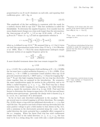
295. 280 Ion traps
prize lecture of Wolfgang Paul.38
The National Physical Laboratory in
38
On the web site of the Nobel prizes.
the UK and the National Institute of Standards and Technology in the
US provide internet resources on the latest developments and research.
Exercises
(12.1) The vibrational modes of trapped ions
Two calcium ions in a linear Paul trap lie in a line
along the z-axis.
(a) The two end-cap electrodes along the z-axis
produce a d.c. potential as in eqn 12.23, with
a2 = 106
V m−2
. Calculate ωz.
(b) The displacements z1 and z2 of the two ions
from the trap centre obey the equations
M
..
z1 = −Mω2
z z1 −
e2
/4π0
(z2 − z1)2 ,
M
..
z2 = −Mω2
z z2 +
e2
/4π0
(z2 − z1)2
.
Justify the form of these equations and show
that the centre of mass, zcm = (z1 + z2)/2
oscillates at ωz.
(c) Calculate the equilibrium separation a of two
singly-charged ions.
(d) Find the frequency of small oscillations of the
relative position z = z2 − z1 − a.
(e) Describe qualitatively the vibrational modes
of three ions in the trap, and the relative or-
der of their three eigenfrequencies.39
(12.2) Paul trap
(a) For Hg+
ions in a linear Paul trap with di-
mensions r0 = 3 mm, calculate the maximum
amplitude Vmax of the radio-frequency voltage
at Ω = 2π × 10 MHz.
(b) For a trap operating at a voltage V0 =
Vmax/
√
2, calculate the oscillation frequency
of an Hg+
ion. What happens to a Ca+
ion
when the electrodes have the same a.c. volt-
age?
(c) Estimate the depth of a Paul trap that has
V0 = Vmax/
√
2, expressing your answer as a
fraction of eV0.
(d) Explain why a Paul trap works for both posi-
tive and negative ions.
(12.3) Investigation of the Mathieu equation
Numerically solve the Mathieu equation and plot
the solutions for some values of qx. Give exam-
ples of stable and unstable solutions. By trial and
error, find the maximum value of qx that gives a
stable solution, to a precision of two significant
figures. Explain the difference between precision
and accuracy. [Hint. Use a computer package for
solving differential equations. The method in Ex-
ercise 4.10 does not work well when the solution
has many oscillations because its numerical inte-
gration algorithm is too simple.]
(12.4) The frequencies in a Penning trap
A Penning trap confines ions along the axis by
repulsion from the two end-cap electrodes; these
have a d.c. positive voltage for positive ions that
gives an axial oscillation frequency, as calculated
in Exercise 12.1. This exercise looks at the radial
motion in the z = 0 plane. The electrostatic po-
tential in eqn 12.23 with a2 = 105
V m−2
leads to
an electric field that points radially outwards, but
the ion does not fly off in this direction because
of a magnetic field of induction B = 1 T along the
z-axis.
Consider a Ca+
ion.
(a) Calculate the cyclotron frequency.
(b) Find the magnetron frequency. [Hint. Work
out the period of an orbit of radius r in a
plane perpendicular to the z-axis by assuming
a mean tangential velocity v = E(r)/B, where
E(r) is the radial component of the electric
field at r.]
39They resemble the vibrations of a linear molecule such as CO2, described in Appendix A; however, a quantitative treatment
would have to take account of the Coulomb repulsion between all pairs of ions (not just nearest neighbours).

296. Exercises for Chapter 12 281
(12.5) Production of highly-charged ions in an EBIT
(a) Estimate the accelerating voltage required for
an electron beam voltage that produces hy-
drogenic silicon Si13+
in an EBIT.
(b) Calculate the radius of the first Bohr orbit
(n = 1) in hydrogenic uranium, U+91
.
(c) Calculate the binding energy of the electron in
U+91
and express it as a fraction of the atom’s
rest mass energy Mc2
.
(d) QED effects contribute 3 × 10−5
eV to the
binding energy of the 1s ground configuration
of atomic hydrogen. Express this as a frac-
tion of the hydrogen atom’s rest mass. Esti-
mate the magnitude of the QED contribution
in the ground state of hydrogen-like uranium
U+91
as a fraction of the rest mass. This frac-
tion gives the precision ∆M/M with which
the ion’s mass must be determined in order to
measure QED effects. Discuss the feasibility
of doing this in an ion trap.
Web site:
http://www.physics.ox.ac.uk/users/foot
This site has answers to some of the exercises, corrections and other supplementary information.

297. Quantum computing
13
13.1 Qubits and their
properties 283
13.2 A quantum logic gate 287
13.3 Parallelism in quantum
computing 289
13.4 Summary of quantum
computers 291
13.5 Decoherence and
quantum error
correction 291
13.6 Conclusion 293
Further reading 294
Exercises 294
Quantum computing will be a revolutionary new form of computation in
the twenty-first century, able to solve problems inaccessible to classical
computers. However, building a quantum computer is very difficult, and
so far only simple logic gates have been demonstrated in experiments on
ions in a linear Paul trap. The ideas of quantum computing have also
been tested in experiments using nuclear magnetic resonance (NMR).
In the Paul trap, the ions sit in an ultra-high vacuum (pressure ∼
10−11
mbar) so that collisions rarely happen, and the ions are well iso-
lated from the environment. We have seen that these conditions enable
extremely high-resolution spectroscopy of single ions because of the very
small perturbations to the energy levels. Quantum computing requires
more than one ion in the trap, and all of these ions must be cooled to the
lowest vibrational level to give a well-defined initial quantum state for
the system.1
This presents a much greater experimental challenge than
1
Quantum computing requires precise
control of the motion of the ions, i.e.
their external degrees of freedom, as
well as their internal state |F, MF .
the laser cooling of a single ion to reduce Doppler broadening, but it has
been achieved in some experiments. The previous chapter describes the
physics of the linear Paul trap but for the purposes of this chapter we
simply assume that the trap produces a harmonic potential with strong
confinement in the radial direction, so that the ions lie in a line along its
z-axis, as shown in Fig. 13.1; their mutual electrostatic repulsion keeps
the ions far enough apart for them to be seen separately.
Fig. 13.1 A string of four ions in a linear Paul trap. Coulomb repulsion keeps the
ions apart and the gap corresponds to an ion in the dark state. In this experiment
two laser beams simultaneously excite strong and weak transitions to give quantum
jumps, as described in Section 12.6, so that each ion flashes on and off randomly. This
snapshot of the system at a particular time could be taken to represent the binary
number 1101. A quantum logic gate requires much more sophisticated techniques in
which laser pulses determine precisely the initial state of each individual ion in the
chain, as described in this chapter. Courtesy of Professors A. M. Steane and D. N.
Stacey, D. M. Lucas and co-workers, Physics department, University of Oxford.

298. 13.1 Qubits and their properties 283
13.1 Qubits and their properties
Fig. 13.2 The two hyperfine levels in
the ground state of an ion. Gener-
ally, experiments use an ion with to-
tal angular momentum J = 1/2 in the
lowest electronic configuration, so that
F = I ± 1/2. The qubits |0 and |1
correspond to two particular Zeeman
states in the two levels, e.g. |F, M and
|F + 1, M, respectively.
A classical computer uses bits with two values 0 or 1 to represent binary
numbers, but a quantum computer stores information as quantum bits
or qubits (pronounced Q-bits). Each qubit has two states, labelled |0
and |1 in the Dirac ket notion for quantum states. Most theoretical
discussions of quantum computing consider the qubit as a spin-1/2 ob-
ject, so the two states correspond to spin down |ms = −1/2 and spin up
|ms = +1/2 . However, for a trapped ion the two states usually corre-
spond to two hyperfine levels of the ground configuration, as illustrated
in Fig. 13.2. In the following discussion, |1 represents the ion in the
upper hyperfine level and |0 is used for the lower hyperfine level, but
all of the arguments apply equally well to spin-1/2 particles since the
principles of quantum computing clearly do not depend on the things
used as qubits. Ions, and other physical qubits, give a compact way of
storing information, e.g. |1101 represents the binary number 1101 in
Fig. 13.1, but the quantum features of this new way of encoding infor-
mation only become apparent when we consider the properties of more
than one qubit in Section 13.1.1. Even though a single qubit gener-
ally exists in a superposition of the two states, a qubit does not carry
more classical information than a classical bit, as shown by the following
argument. The superposition of the two states
ψqubit = a|0 + b|1 (13.1)
obeys the normalisation condition |a|2
+ |b|2
= 1 . We write this super-
position in the general form
ψqubit =
cos
θ
2
|0 + eiφ
sin
θ
2
|1
eiφ
. (13.2)
The overall phase factor has little significance and the possible states cor-
respond to vectors of unit length with direction specified by two angles θ
and φ. These are the position vectors of points lying on the surface of a
sphere, as in Fig. 13.3. The state |0 lies at the north pole of this Bloch
sphere and |1 at the south pole; all other position vectors are superpo-
sitions of these two basis states. Since these position vectors correspond
to a simple classical object such as a pointer in three-dimensional space,
it follows that the information encoded by each qubit can be modelled
in a classical way.
The analogy between a qubit and a three-dimensional pointer seems to
imply that a qubit stores more information than a bit with two possible
values 0 or 1, e.g. like one of the hands of an analogue clock that gives us
information about the time by its orientation in two-dimensional space.
Generally, however, this is not true because we cannot determine the ori-
entation of a quantum object as precisely as the hands on a clock. Mea-
surements can only distinguish quantum states, with a high probability,
if the states are very different from each other, occupying well-separated
positions on opposite sides of the Bloch sphere. A measurement on a

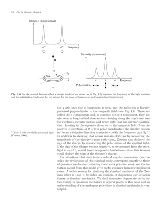
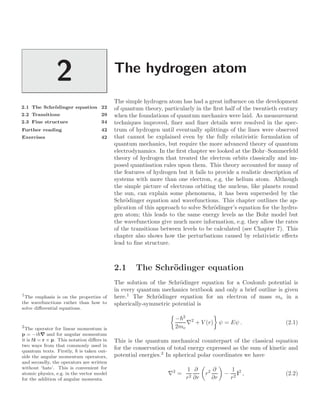
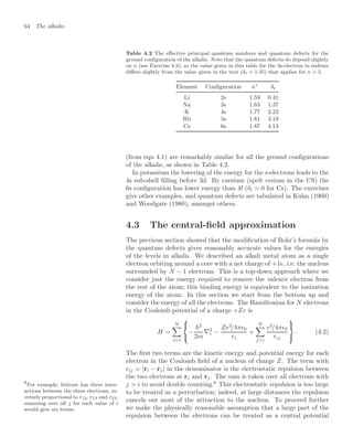
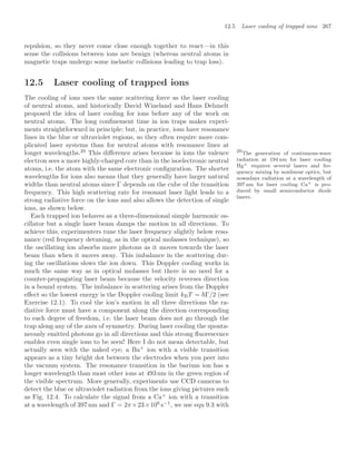
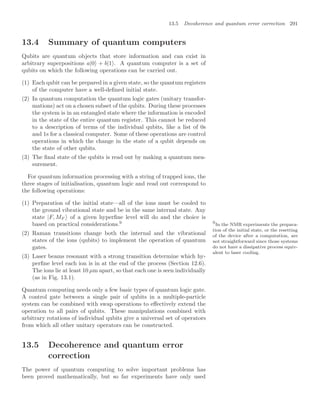
299. 284 Quantum computing
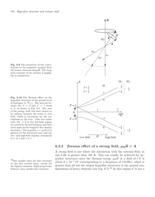
Fig. 13.3 The state |0 lies at the
north pole of this Bloch sphere and
|1 at the south pole; all other posi-
tion vectors are superpositions of these
two basis states. The Bloch sphere
lies in the Hilbert space spanned by
the two eigenvectors |0 and |1. The
Hadamard transformation defined in
eqn 13.3 takes |0 → |0 + |1 (cf.
Fig. 7.2).
spin-1/2 particle determines whether its orientation is up or down along
a given axis. After that measurement the particle will be in one of those
states since the act of measurement puts the system into an eigenstate
of the corresponding operator. In the same way, a qubit will give either
0 or 1, and the read-out process destroys the superposition.
The Bloch sphere is very useful for describing how individual qubits
transform under unitary operations. For example, the Hadamard trans-
formation that occurs frequently in quantum computation (see the ex-
ercises at the end of this chapter) has the operator2
2
In this chapter wavefunctions are writ-
ten without normalisation, which is the
common convention in quantum com-
putation.
ÛH |0 → |0 + |1 ,
ÛH |1 → |0 − |1 .
(13.3)
This is equivalent to the matrix
ÛH =
1
√
2
1 1
1 −1
.
The effect of this unitary transformation of the state is illustrated in
Fig. 13.3—it corresponds to a rotation in the Hilbert space containing
the state vectors. This transformation changes |0 , at the north pole,
into the superposition given in eqn 13.3 that lies on the equator of the
sphere.
13.1.1 Entanglement
We have already encountered some aspects of the non-intuitive behaviour
of multi-particle quantum systems in the detailed description of the two
electrons in the helium atom (Chapter 3), where the antisymmetric spin
state [ |↓↑ − |↑↓ ]/
√
2 corresponds to the wavefunction
Ψ = |01 − |10 (13.4)
in the notation used in this chapter (without normalisation). This does
not factorise into a product of single-particle wavefunctions:
Ψ = ψ1ψ2 , (13.5)

300. 13.1 Qubits and their properties 285
where
ψ1ψ2 = [ a|0 + b|1 ]1 [ c|0 + d|1 ]2 . (13.6)
Here c and d are additional arbitrary constants, and the futility of at-
tempting to determine these constants quickly becomes obvious if you
try it. Generally, we do not bother with the subscript used to denote the
particle, so |0 1|1 2 ≡ |01 and |1 1|1 2 ≡ |11 , etc. Multiple-particle sys-
tems that have wavefunctions such as eqn 13.4 that cannot be written as
a product of single-particle wavefunctions are said to be entangled. This
entanglement in systems with two, or more, particles leads to quantum
properties of a completely different nature to those of a system of clas-
sical objects—this difference is a crucial factor in quantum computing.
Quantum computation uses qubits that are distinguishable, e.g. ions at
well-localised positions along the axis of a linear Paul trap. We can label
the two ions as Qubit 1 and Qubit 2 and know which one is which at any
time. Even if they are identical, the ions remain distinguishable because
they stay localised at certain positions in the trap. For a system of dis-
tinguishable quantum particles, any combination of the single-particle
states is allowed in the wavefunction of the whole system:
Ψ = A|00 + B|01 + C|10 + D|11 . (13.7)
The complex amplitudes A, B, C and D have arbitrary values. It is
convenient to write down wavefunctions without normalisation, e.g.
Ψ = |00 + |01 + |10 + |11 , (13.8)
Ψ = |00 + 2|01 + 3|11 , (13.9)
Ψ = |01 + 5|10 . (13.10)
Two of these three wavefunctions possess entanglement (see Exercise
13.1). We encounter examples with three qubits later (eqn 13.12).
In the discussion so far, entanglement appears as a mathematical prop-
erty of multiple-particle wavefunctions, but what does it mean physi-
cally? It is always dangerous to ask such questions in quantum me-
chanics, but the following discussion shows how entanglement relates
to correlations between the particles (qubits), thus emphasising that
entanglement is a property of the system as a whole and not the indi-
vidual particles. As a specific example consider two trapped ions. To
measure their state, laser light excites a transition from state |1 (the
upper hyperfine level) to a higher electronic level to give a strong flu-
orescence signal, so |1 is a ‘bright state’, while an ion in |0 remains
dark.3
Wavefunctions such as those in eqns 13.4 and 13.10 that contain 3
This is similar to the detection of
quantum jumps in Section 12.6, but
typically quantum computing experi-
ments use a separate laser beam for
each ion to detect them independently.
only the terms |10 and |01 always give one bright ion and the other
dark, i.e. an anticorrelation where a measurement always finds the ions
in different states. To be more precise, this corresponds to the following
procedure. First, prepare two ions so that the system has a certain ini-
tial wavefunction Ψin, then make a measurement of the state of the ions
by observing their fluorescence. Then reset the system to Ψin before
another measurement. The record of the state of the ions for a sequence

301. 286 Quantum computing
of such measurements looks like: 1 0, 1 0, 0 1, 1 0, 1 0, . . .. Each ion
gives a random sequence of 0s and 1s but always has the opposite state
to the other ion.
This example does not illustrate the full subtlety of entanglement be-
cause we would get the same result if we prepared the two ions either
in |01 or |10 randomly at the beginning. Such an apparatus produces
correlated pairs of ions in a purely classical way that mimics the quan-
tum situation. John Bell proved that we can make measurements that
distinguish the ‘classical correlation’ from an entangled state. The above
description shows that this cannot be done simply by making measure-
ments along the axes defined by the basis states |0 and |1 , but it turns
out that quantum entanglement and ‘classically-correlated’ particles give
different results for measurements along other sets of axes. This was a
very profound new insight into the nature of quantum mechanics that
has stimulated much important theoretical and experimental work.4
4
Bell considered the well-known EPR
paradox and the system of two ions de-
scribed above has the same properties
as the two spin-1/2 particles usually
used in quantum mechanics texts (Rae
1992).
‘Entanglement implies correlation but correlation does not imply en-
tanglement’. In the following we shall concentrate mainly on the first
half of this statement, i.e. two-particle systems encode quantum infor-
mation as a joint property of the qubits and carry more information than
can be stored on the component parts separately. The quantum infor-
mation in an entangled state is very delicate and is easily destroyed by
perturbations of the relative phase and amplitude of the qubits, e.g. in
present-day ion traps it is difficult to maintain coherence between more
than a few qubits; this decoherence is caused by random perturbations
that affect each qubit in a different way.
The wavefunctions of the two electrons in helium are entangled but
they do not give qubits useful for quantum computing. Nevertheless,
since this is a book about atomic physics it is worthwhile to look back
at helium. The antisymmetric state of the two spins has already been
used as an example of entanglement. The symmetric spin wavefunction
[ |↓↑ + |↑↓ ]/
√
2 also has entanglement, but the two other symmetric
wavefunctions factorise: |↑↑ ≡ |↑ 1|↑ 2, and similarly for |↓↓ . The two
electrons are in these eigenstates of S because of the exchange symme-
try. When the two electrons do not have the same quantum numbers, n
and l, the spatial wavefunctions are symmetric and antisymmetric com-
binations of the single-electron wavefunctions and are entangled. These
eigenstates of the residual electrostatic interaction also satisfy the re-
quirement of exchange symmetry for identical particles. (Note that the
energy levels and spatial wavefunctions would be the same even if the
particles were not identical—see Exercise 3.4.) The exchange integrals
in helium can be regarded as a manifestation of the entanglement of the
spatial wavefunction of the two electrons that leads to a correlation in
their positions, or an anticorrelation, making it more (or less) probable
that the electrons will be found close together. From the quantum per-
spective, the energy difference for two different entangled wavefunctions
does not seem strange because we do not expect them to have the same
properties, even if they are made up of the same single-electron states.

302. 13.2 A quantum logic gate 287
13.2 A quantum logic gate
Quantum computing uses nothing more than standard quantum mechan-
ics but it combines operations on the qubits and quantum measurements
in sophisticated ways to give amazingly powerful new methods for com-
putation. Here we consider just one example of the transformations of
the qubits, or quantum logic gates, that form the elementary building
blocks (primitives) of a quantum computer. The controlled-NOT gate
(CNOT) transforms two qubits, as shown in Table 13.1.
The CNOT gate changes the value of the second qubit if and only
if the first qubit has the value 1. The first qubit controls the effect
of the gate on the second qubit. The truth Table 13.1 looks the same
as that for ordinary logic, but a quantum logic gate corresponds to
an operation that preserves the superposition of the input states. The
quantum mechanical operator of the CNOT gate ÛCNOT acts on the
wavefunction of the two qubits to give
ÛCNOT {A |00 + B |01 + C |10 + D |11 }
→ A |00 + B |01 + C |11 + D |10 .
(13.11)
Alternatively, the effect of this operation can be written as |10 ↔ |11 ,
with the other states unchanged. The complex numbers A, B, C and D
represent the phase and relative amplitude of states within the super-
position.
13.2.1 Making a CNOT gate
The CNOT gate is elementary but it turns out not to be the simplest
gate to make in an ion trap quantum processor—it requires a sequence
of several operations, as described in Steane (1997). So, despite the
fact that quantum computing has been introduced into this book as an
application of ion trapping, this section explains how to make a quan-
tum logic gate for two spin-1/2 particles. This two-qubit system is not
just a convenient theoretical case, but corresponds to actual quantum
computing experiments carried out with the nuclear magnetic resonance
(NMR) technique. Figure 13.4 shows the energy levels of the two inter-
acting spins.
We do not need to go into all the details of how this energy-level struc-
ture arises to understand how to make a CNOT gate, but it is important
Table 13.1 Truth table of the CNOT quantum logic gate.
|00 → |00
|01 → |01
|10 → |11
|11 → |10

303. 288 Quantum computing
(b)
(a)
Energy
Fig. 13.4 (a) The energy levels of two spin-1/2 particles which do not interact with each other. The frequencies that drive
the transition between the levels of Qubit 1 and Qubit 2 are ω1 and ω2, respectively. In NMR these levels correspond to the up
and down orientations of two protons in a strong magnetic field, i.e. the states |mI = ±1/2 for each proton. The difference in
the resonance frequencies ω1 = ω2 arises from interaction with their surroundings (other nearby atoms in the molecule). (b)
The energy levels of two interacting particles, or qubits. The interaction between the qubits makes the frequency required to
change the orientation of Qubit 2 depend on the state of the other qubit (and similarly for Qubit 1). To denote this, the two
new resonance frequencies close to ω2 are labelled with the superscripts |0x and |1x. (Note this rather cumbersome notation
is not generally used but it is useful in this introductory example.) The absorption spectrum is drawn below the corresponding
transitions. A π-pulse of radio-frequency radiation at angular frequency ω
|1x
2 switches Qubit 2 (|02 ↔ |12) if and only if
Qubit 1 is in |11. This gives the CNOT gate of Table 13.1. For details of the NMR technique see Atkins (1994). In NMR the
interaction of the nuclear magnetic moment with a strong external magnetic field gI µBI · B dominates. For a field of 10 T the
protons at the centre of the hydrogen atoms in the sample have resonance frequencies of 400 MHz. This frequency corresponds
to approximately ω1/2π ω2/2π in the figure. The chemical shift causes ω1 and ω2 to differ by only a few parts per million,
but this is resolved by standard NMR equipment. Atkins (1994) describes how the fine structure in NMR spectra, shown in
(b), arises from spin–spin coupling between the two nuclear spins.
to know that spontaneous emission is negligible.5
To make our discussion
5
The amplitudes and phases of the
states within the superposition must
not change spontaneously, i.e. the de-
coherence must be very small over the
time-scale of the experiment.
less abstract, it is also useful to know that in NMR experiments the
energy differences between the levels shown in Fig. 13.4 arise from the
orientation of the magnetic moment of the nuclei, proportional to their
spin, in a strong magnetic field and that radio-frequency radiation drives
transitions between the states. There is a splitting of ω1 between the
up and down states of the first qubit (|0 and |1 ) and ω2 for the
second qubit. Therefore a pulse of radio-frequency radiation at angular
frequency ω1 changes the orientation of the first spin (Qubit 1); for
example, a π-pulse (as defined in Section 7.3.1) swaps the states of this

304. 13.3 Parallelism in quantum computing 289
qubit |0 ↔ |1 , i.e. a|0 +b|1 → a|1 +b|0 . Similarly, pulses at angular
frequency ω2 manipulate the state of the other spin (Qubit 2). These
changes in the state of each qubit independently are not sufficient for
quantum computing. The qubits must interact with each other so that
one qubit ‘controls’ the other qubit and influences its behaviour. A
small interaction between the spin causes the shift of the energy levels
indicated in going from Fig. 13.4(a) to (b)—the energy required to flip
Qubit 2 now depends on the state of Qubit 1 (and vice versa). The energy
levels in Fig. 13.4(b) give four separate transition frequencies between
the four states of the two qubits; a pulse of radio-frequency radiation
that drives one of these transitions can achieve the CNOT operation—it
changes the state of Qubit 2 only if Qubit 1 has state |1 .6 6
The coupling between trapped ions
arises from the mutual electrostatic re-
pulsion of the ions, but this interaction
between qubits does not give a level
structure like that in Fig. 13.4.
Although it seems simple for the spin-1/2 system, the implementa-
tion of a quantum logic gate represents a major step towards building
a quantum computer. Rigorous proofs based on mathematical proper-
ties of unitary operators in quantum mechanics show that any unitary
operation can be constructed from a few basic operators—it is sufficient
to have just one gate which gives control of one qubit by another, such
as the CNOT, in addition to the ability to manipulate the individual
qubits in an arbitrary way.7
These operators form a so-called universal
7
To rotate the nuclear spins to an ar-
bitrary point on the Bloch sphere the
NMR experiments use radio-frequency
pulses. Experiments in ion traps use
Raman pulses (Section 9.8).
set which generates all other unitary transformations of the qubits.
13.3 Parallelism in quantum computing
A classical computer acts on binary numbers stored in the input regis-
ter, or registers, to output another number also represented as bits with
values 0 and 1. A quantum computer acts on the whole superposition of
all the input information in the qubits of its input register, e.g. a string
of ions in a linear Paul trap. This quantum register can be prepared
in a superposition of all possible inputs at the same time, so that the
quantum computing procedure transforms the entire register into a su-
perposition of all possible outputs. For example, with N = 3 qubits a
general initial state containing all possible inputs has the wavefunction
Ψ = A |000 + B |001 + C |010 + D |011
+ E |100 + F |101 + G |110 + H |111 .
(13.12)
Quantum computing corresponds to carrying out a transformation, rep-
resented by the quantum mechanical operator Û, to give the wavefunc-
tion Ψ
= ÛΨ that is a superposition of the outputs corresponding to
each input
Ψ = AÛ |000 + BÛ |001 + CÛ |010 + . . . . (13.13)
Useful quantum algorithms combine different operations, such as
ÛCNOT, to give an overall transformation Û = Ûm · · · Û2Û1, and these
operations have the same advantage of parallelism as for the individ-
ual operations. It appears that, instead of laboriously calculating the
output for each of the binary numbers 000 to 111, corresponding to 0

305. 290 Quantum computing
to 7 in decimals, the quantum computation does all eight calculations
simultaneously. Herein lies the great power of quantum computing.
The number of combinations of the input states increases exponen-
tially with the number of qubits; for a register of 100 qubits this means
a transformation of 2100
≡ 1030
inputs in parallel—an astronomical num-
ber. But how can the correct answer be picked out from the enormous
number of possible outputs? All the possibilities encoded in the multiple-
particle wavefunction Ψ
cannot be turned into a list of the outputs for
a given input, as given by a classical computer. Indeed, a simple quan-
tum measurement just gives one of the outputs chosen randomly from
all the possibilities. However, quantum mechanics allows measurements
that give some information about all of the outputs, if we renounce the
possibility of getting information about any particular output—just as
the complementarity principle stops us knowing both the position and
momentum of a particle precisely. As a trivial example that gives the
flavour of this idea, but is in fact not strictly correct, consider the mea-
surement of the state of the last qubit in the output register—if all the
possible outputs are even numbers then this ion will be in |0 . So we
can establish something about all the possibilities in a single quantum
computation, but this does not allow any more information to be ex-
tracted, i.e. if they are not all even we cannot find out which ones are
odd (nor which input states gave these outputs). Similar ideas apply for
more complicated quantum algorithms, e.g. finding the prime factors of
numbers. (The real nature of quantum computation can only properly
be appreciated by working through a quantum example, so the grossly
simplified case given here must not be pushed too far.)
The factorisation of large numbers is often quoted as a ‘killer appli-
cation’ of quantum computing, i.e. something that they can do which
cannot be done on existing computers (within a realistic time). It is ob-
viously easy to multiply two prime numbers together, e.g. 37×61 = 2257;
but it is much more difficult to go in the opposite direction, e.g. to find
the prime factors of 1271 (try it for yourself). For the larger numbers a
classical computer can easily do the multiplication, but the factorisation
of a number of order 10100
would take an exceedingly long time even with
the fastest supercomputers and the most efficient classical algorithm to
search for the prime factors. It has been proved rigorously that quantum
algorithms exist to attack this type of problem—the algorithms act like
a filter only letting through the sought-after combination of qubits from
the input superposition state. The practical impossibility of factorising
large numbers on present-day computers forms the foundation of the
best methods of encryption.8
A quantum computer has the ability to
8
The need for safe methods of encrypt-
ing information has always been cru-
cial for the military, and nowadays it
is important for confidential electronic
transfer of data in business and to pro-
tect credit card numbers.
try many combinations in each computation and so quickly find the key.
The possibility of cracking the best currently-used codes has prompted
such hard-headed bodies as the government security agencies to investi-
gate quantum computing and fund research on ion traps. One wonders
what they think of the intrigue and mystery of quantum mechanics.

306. 13.5 Decoherence and quantum error correction 291
13.4 Summary of quantum computers
Qubits are quantum objects that store information and can exist in
arbitrary superpositions a|0 + b|1 . A quantum computer is a set of
qubits on which the following operations can be carried out.
(1) Each qubit can be prepared in a given state, so the quantum registers
of the computer have a well-defined initial state.
(2) In quantum computation the quantum logic gates (unitary transfor-
mations) act on a chosen subset of the qubits. During these processes
the system is in an entangled state where the information is encoded
in the state of the entire quantum register. This cannot be reduced
to a description of terms of the individual qubits, like a list of 0s
and 1s for a classical computer. Some of these operations are control
operations in which the change in the state of a qubit depends on
the state of other qubits.
(3) The final state of the qubits is read out by making a quantum mea-
surement.
For quantum information processing with a string of trapped ions, the
three stages of initialisation, quantum logic and read out correspond to
the following operations:
(1) Preparation of the initial state—all of the ions must be cooled to
the ground vibrational state and be in the same internal state. Any
state |F, MF of a given hyperfine level will do and the choice is
based on practical considerations.9 9
In the NMR experiments the prepara-
tion of the initial state, or the resetting
of the device after a computation, are
not straightforward since those systems
do not have a dissipative process equiv-
alent to laser cooling.
(2) Raman transitions change both the internal and the vibrational
states of the ions (qubits) to implement the operation of quantum
gates.
(3) Laser beams resonant with a strong transition determine which hy-
perfine level each ion is in at the end of the process (Section 12.6).
The ions lie at least 10 µm apart, so that each one is seen individually
(as in Fig. 13.1).
Quantum computing needs only a few basic types of quantum logic gate.
A control gate between a single pair of qubits in a multiple-particle
system can be combined with swap operations to effectively extend the
operation to all pairs of qubits. These manipulations combined with
arbitrary rotations of individual qubits give a universal set of operators
from which all other unitary operators can be constructed.
13.5 Decoherence and quantum error
correction
The power of quantum computing to solve important problems has
been proved mathematically, but so far experiments have only used

307. 292 Quantum computing
a few qubits to demonstrate the principle of some elementary opera-
tions. These experiments all use state-of-the-art techniques, but for
large systems the external perturbations blur the entangled states so
that they cannot be distinguished from each other, e.g. for ions in the
Paul trap the electrical noise on the radio-frequency electrodes causes
random changes of the phase of the states within a superposition. In the
year 2000 the best ion trap experiment was limited to four qubits.10
De-
10
At that time NMR experiments used
up to seven qubits. coherence quickly causes a system of many qubits to become so muddled
up that it is impossible to pick out the required output. In contrast, in a
classical computer errors which change 0 into 1, or the other way round,
occur extremely rarely, and present-day computers have procedures for
correcting errors so that they have a negligible effect.
Decoherence was thought to be an incurable disease in real quan-
tum systems that would prevent quantum information processing from
ever being carried out with enough qubits to make it really useful. How-
ever, a new cunning way of encoding information has been invented that
cures the symptoms of decoherence. So-called quantum error correction
(QEC) exploits the subtle features of the theory of quantum mechanics
to get rid of the small amounts of the unwanted states that gradually
get mixed into the states containing the quantum information by per-
turbations on the system. Broadly speaking, making a certain type of
quantum measurement causes the wavefunction of the system of qubits
to ‘collapse’, in a way that destroys any additional phase or amplitude in-
troduced by decoherence. This measurement must be made with respect
to a very carefully chosen basis of eigenstates to preserve the entangle-
ment of the wavefunction. Clearly, it is not adequate to make a simple
measurement that causes quantum superpositions to collapse into just
one of the states within the superposition, since this would completely
destroy the coherence between the states that we want to preserve.11
11
QEC manages to make measure-
ments on eigenstates that are in some
sense orthogonal to those in the origi-
nal superposition. These special quan-
tum measurements cause the small ad-
mixture of other states introduced into
the wavefunction by the noise to col-
lapse to zero. The QEC measurements
are performed on extra qubits entan-
gled with the qubits in the quantum
register; measurements made on these
ancillary qubits do not reduce the size
of the superposition state that stores
quantum information (in the register),
i.e. the number of qubits in the su-
perposition is preserved in QEC. The
technical details of this process are ex-
plained in Steane (1998). Some elemen-
tary aspects of QEC can be appreciated
by analogy with the quantum Zeno ef-
fect described in Exercise 13.5.
In the context of ion traps, the recent advances in quantum com-
puting and QEC can be regarded as the latest steps in the evolution
of spectroscopy and laser cooling, as illustrated by the following rough
history.
(1) The first spectroscopists observed light from discharge lamps, e.g.
the Balmer lines in atomic hydrogen. They used spectrographs and
étalons and the resolution was limited by Doppler broadening, to-
gether with collisions and other broadening mechanisms in the dis-
charge.
(2) Atomic beams allowed experimenters to change the population be-
tween the various energy levels of the atoms, using radio-frequency
or microwave radiation to manipulate hyperfine and Zeeman levels
in the ground state. (Optical pumping was applied to the ground
states of certain atoms.) Atoms were deflected slightly in the Stern–
Gerlach experiment but without a significant change in speed. The
laser extended these techniques to the higher levels using optical
transitions, so that, in principle, atomic physics experiments can
manipulate the internal states of the atoms and put atoms into any

308. 13.6 Conclusion 293
desired energy level.
(3) Ion traps confined the ions for long periods with buffer gas cooling.
(4) The advent of laser cooling of atoms meant that spectroscopists were
no longer passive observers, but could magnetically trap neutral
atoms and control the atom’s motion. Laser cooling of ions can put
them into the ground state of the trap to give a completely defined
external state.
(5) Quantum computing techniques allow the manipulation of both the
external and internal state of the trapped ion qubits with laser light,
to put a system of many ions into a particular quantum state.
(6) Quantum error correction can be regarded as a refined form of laser
cooling. QEC puts the ions back into a coherent superposition of
the desired states of the system (actually a particular sub-space of
Hilbert space), rather than the lowest energy state as in conven-
tional cooling. It was a real surprise that decoherence in quantum
mechanics can be overcome in this way and actively stabilise quan-
tum information.
13.6 Conclusion
At heart, quantum mechanics remains mysterious. Certain aspects of
quantum behaviour seem strange to our intuition based on the classi-
cal world that we experience directly, e.g. the well-known examples of
‘which way the photon goes’ in a Young’s double-slit experiment and
Schrödinger’s cat paradox.12
These examples have provoked much dis- 12
See quotation from Heisenberg in the
background reading section of the Pref-
ace.
cussion and thought over the years about the so-called quantum mea-
surement problem. Nowadays, physicists do not regard the peculiarities
of quantum systems as a problem at all, but rather as an opportunity.
A proper appreciation of the profoundly different properties of multiple-
particle systems and the nature of entanglement has shown how to use
their unique behaviour in quantum computing. Just as a car mechanic
uses her practical knowledge to get an engine working, without worry-
ing about the details of internal combustion, so a quantum mechanic
(or quantum state engineer) can design a quantum computer using the
known rules of quantum mechanics without worrying too much about
philosophical implications. Physicists, however, strive towards a bet-
ter understanding of the quantum world and consideration of the pro-
found and subtle ideas in quantum information theory sheds new light
on aspects of quantum mechanics. In physics research there often exists
a symbiotic relationship between theory and experimental work, with
each stimulating the other; a prime example is quantum error correc-
tion which was not thought about until people started to face up to
the fact that none of the systems used in existing experiments has any
possibility of working reliably with a useful number of qubits (without
error correction)—of course, the problem of decoherence has always been
recognised but experimental results focused attention on this issue.

309. 294 Quantum computing
The theoretical principles of quantum computing are well understood
but there are many practical difficulties to overcome before it becomes
a reality. All potential systems must balance the need to have interac-
tions between the qubits to give coherent control and the minimisation
of the interactions with the external environment that perturb the sys-
tem. Trapped ions have decoherence times much longer than the time
needed to execute quantum logic gates and this makes them one of the
most promising possibilities. In quantum computing many new and in-
teresting multiple-particle systems have been analysed and, even if they
cannot be realised yet, thinking about them sharpens our understand-
ing of the quantum world, just as the EPR paradox did for many years
before it could be tested experimentally.
Further Reading
The Contemporary Physics article by Cummins and Jones (2000) gives
an introduction to the main ideas and their implementation by NMR
techniques. The books by Nielsen and Chuang (2000) and Stolze and
Suter (2004) give a very comprehensive treatment. The article on the
ion-trap quantum information processor by Steane (1997) is also useful
background for Chapter 12. Quantum computing is a fast-moving field
with new possibilities emerging all the time. The latest information can
be found on the World-Wide Web.
Exercises
(13.1) Entanglement
(a) Show that the two-qubit state in eqn 13.8 is
not entangled because it can be written as a
simple product of states of the individual par-
ticles in the basis |0
= (|0 − |1)/
√
2 and
|1
= (|0 + |1)/
√
2.
(b) Write the maximally-entangled state |00 +
|11 in the new basis.
(c) Is |00 + |01 − |10 + |11 an entangled state?
[Hint. Try to write it in the form of eqn 13.6
and find the coefficients.]
(d) Show that the two states given in eqns 13.9
and 13.10 are both entangled.
(e) Discuss whether the three-qubit state Ψ =
|000 + |111 possesses entanglement.
(13.2) Quantum logic gates
This question goes through a particular example
of the statement that any operation can be con-
structed from a combination of a control gate and
arbitrary rotations of the individual qubits. For
trapped ions the most straightforward logic gate
to build is a controlled ‘rotation’ of Qubit 2 when
Qubit 1 is |1, i.e.
ÛCROT {A |00 + B |01 + C |10 + D |11}
= A |00 + B |01 + C |10 − D |11 .

310. Exercises for Chapter 13 295
(a) Write ÛCROT as a 4 × 4 matrix and show that
it is unitary.
(b) Equation 13.3 defines the Hadamard transfor-
mation. Write this transformation for Qubit
2, ÛH(2) as a 4×4 matrix with the same basis
states as in (a), and show that it is unitary.
(c) Find the combination of ÛCROT, ÛH(2) and
Û†
H(2) that gives the CNOT gate (Table 13.1).
(13.3) Elementary operations with more than two qubits
The CNOT gate where the state of Qubit 1 con-
trols whether Qubit 2 switches (Table 13.1) cor-
responds to the operator ÛCNOT(1, 2). Note that
ÛCNOT(1, 2) = ÛCNOT(2, 1) and that these gates
do not affect other qubits.
(a) A system of three qubits has a quantum bus
that enables operations that swap the states
of any pair of qubits: ÛSWAP(1, 2) for 1 ↔ 2,
ÛSWAP(2, 3) for 2 ↔ 3 and ÛSWAP(1, 3) for
1 ↔ 3. What combination of ÛCNOT(1, 2) and
SWAP operators gives ÛCNOT(1, 3), a CNOT
gate where Qubit 1 controls Qubit 3?
(b) The operator ÛH(i) gives the transforma-
tion |0 → (|0 + |1)/
√
2 for the ith qubit.
Show that ÛH(3)ÛH(2)ÛH(1) acting on |000
gives the three-qubit state with all coefficients
equal, namely A = B = C = D = E = F =
G = H in eqn 13.12.
(c) The three operations in part (b) prepare eight
input states, i.e. they put a three-qubit reg-
ister into a superposition of the eight states.
How many inputs are prepared by thirty such
operations on thirty qubits. Is the initial state
of the quantum register prepared in this way
entangled?
(13.4) Grover’s search algorithm
Imagine trying to find a given number in the tele-
phone directory when you have written down the
number but not the name. There is no clever clas-
sical way of speeding up this tedious task but the
massive parallelism of a quantum algorithm does
make a big difference to this sort of problem. In
this question we consider finding a particular value
of a two bit number x from the list of four possibil-
ities, but the principles can be extended to larger
numbers. To implement the search the quantum
computer uses an operation in which the sign of
the input changes for the specified value—if we
assume the answer is x = |11 then the operation
causes |11 → −|11 but leaves the other states
unchanged. Instead of a simple list, the assign-
ment of x could be made on the basis of a so-
lution to an algebraic problem, e.g. the operator
changes the sign of the input x if some function of
x has a particular value such as f(x) = 0. In order
that the computer can implement the sign change
efficiently it is only necessary that the function
f(x) can be evaluated efficiently for some general
x. This is a much easier task than finding the value
of x for which f(x) = 0.
The figure shows the sequence of operations corre-
sponding to Grover’s algorithm, starting with two
qubits in |00. The operators are defined in the fol-
lowing. The letters (a) to (f) indicate the part of
this question corresponding to each stage. (Ignore
normalisation factors throughout this question.)
(a) Show that the Hadamard transformation
(eqn 13.3) applied to each of the qubits of |00
results in the superposition state
Ψin = |00 + |01 + |10 + |11 .
This is the initial state of the two qubits
needed for the algorithm.
(b) The box labelled f(x) represents the oper-
ation for the function, as described above.
In this question this corresponds to a CROT
gate (defined in Exercise 13.2). Write down
ÛCROTΨin.
(c) The next step in the algorithm is another
Hadamard transformation of each qubit. We
have already worked out the effect on |00
in part (a). Work out the effect on |01,
|10 and |11. Show that the superposition
is |00 + |01 + |10 − |11.

311. 296 Quantum computing
(d) The operator ÛZ corresponds to |0 → |0 and
|1 → −|1, for each qubit. Write down the
resulting state of the system of two qubits.
(e) Show that after another ÛCROT the state is
|00 − |01 − |10 + |11 .
(f) Show that a final Hadamard transformation
yields the required answer.
(g) Repeat the algorithm for another function
with solution x = 10, to show that it picks
out the required value, i.e. f(x) corresponds
to |10 → −|10.
Comment. This algorithm has a similar ‘one-way’
nature to the factorisation of numbers mentioned
in the text—it is very time consuming to find the
prime factors, but once possible solutions have
been found by the quantum computation it is easy
to verify whether they are indeed factors (or satisfy
the equation) using a classical computer. Some
more complex quantum algorithms do not always
give the ‘correct’ answer but they are still useful
in ‘winnowing the wheat from the chaff’; the al-
gorithms pick out all the required answers (grains
of wheat) along with a few unwanted numbers.
This is not a problem since invalid numbers are
thrown away after checking—the set of numbers
to be checked is much smaller than the initial set
of all possibilities, so the procedure is efficient.
(13.5) The quantum Zeno effect
The ancient Greek philosopher Zeno proposed var-
ious arguments against motion, e.g. Achilles and
the tortoise in which the logic leads to the para-
doxical conclusion that the man cannot overtake
the tortoise. In the quantum Zeno effect the evo-
lution of a wavefunction is slowed down by re-
peated quantum measurements on the system, and
this has been described by the colloquial phrase ‘a
watched pot never boils’.
This question is based on the usual treatment of
Rabi oscillations rewritten in terms of the states of
a qubit that starts in |0 at time t = 0. Transitions
between the states are induced by a perturbation
which is characterised by the Rabi frequency Ω:
|ψ = cos
Ωt
2
|0 − i sin
Ωt
2
|1 .
(a) The state of the qubit is measured after a short
time τ 1/Ω. Show that the probability that
the qubit ends up in |1 is (Ωτ/2)2
1. What
is the probability that the qubit is in |0 after
the measurement?
(b) The state of the qubit is measured at time τ/2.
What are now the probabilities of |0 and |1?
(c) After the measurement at time τ/2 the qubit
will be in either |0 or |1. The qubit then
evolves for time τ/2 and its state is measured
again at time τ. Calculate the probability of
the outcome |1.
(d) For a sequence of n measurements with a time
interval of τ/n between them, the probability
of having made a transition from |0 to |1 at
time τ is 1/n times that in part (a). Verify
this result for n = 3 or, if you can, justify it
for the general case.
(e) Discuss the application of these results to the
measurement of the frequency of a narrow
transition by the quantum jump technique, as
described in Section 12.6. The transition rate
on the weak transition decreases as the mea-
surement periods of excitation on the strong
transition become more frequent. What effect
does this have on the measured line width of
the narrow transition?
(13.6) Quantum error correction
Classical computers encode each number with
more than the minimum number of bits neces-
sary; the additional ‘check’ bits allow the system
to detect whether any of the bits has undergone a
random change (caused by noise). In these error
correction codes the binary code for each number
differs from the string of 0s and 1s for any other
possible number by at least two bits, so a random
change of a single bit leads to an invalid binary
code that the computer rejects. In practice, error
correction codes have the binary strings represent-
ing valid entries ‘further apart’ to protect against
errors in several bits. Quantum error correction
(QEC) uses extra qubits to make the computa-
tional states ‘further apart’ (in Hilbert space), so
the system is more robust, i.e. it is harder for the
computational states to become mixed.

312. Exercises for Chapter 13 297
The above figure shows a particular QEC scheme.
On the left-hand side, Qubit 1 starts in |x and
Qubits 2 and 3 both start in |0. The letters (a) to
(d) indicate the part of this question correspond-
ing to each stage.
(a) To represent the qubit |x = a|0 + b|1 this
quantum error correction code uses Ψin =
a|000 + b|111. Show that two CNOT gates
acting on Qubits 2 and 3, with Qubit 1 as the
control qubit in both cases, as indicated in the
figure, encode |x in this way.
(b) Suppose that a perturbation of Qubit 1 causes
a bit-change error so that the state of the
three qubits becomes α(a|000 + b|111) +
β(a|100 + b|011). Here β is the amplitude
of the unwanted state mixed into the origi-
nal state (and normalisation determines α).
Show that after another two CNOT gates we
get (a|0 + b|1) α|00 + (a|1 + b|0) β|11 .
(c) The measurement of the states of Qubits 2
and 3 has two possible results. One possibility
is to find |11, which means that Qubit 1 has
changed and in this case the error is corrected
by applying a (conditional) NOT operation to
Qubit 1, i.e. |0 ↔ |1 if and only if the mea-
surement of the other qubits gives |11. What
is the other possible state of Qubits 2 and 3
resulting from the measurement? Verify that
Qubit 1 ends up in the original state |x after
this stage.
(d) Qubits 2 and 3 are both reset to |0. Two fur-
ther CNOT gates recreate Ψin from |x, just
as in stage (a).
This scheme corrects ‘bit flip’ errors in any of the
qubits. Show this by writing out what happens in
stages (b), (c) and (d) for the state
α (a |000 + b |111) + β (a |100 + b |011)
+ γ (a |010 + b |101) + δ (a |001 + b |110) .
Web site:
http://www.physics.ox.ac.uk/users/foot
This site has answers to some of the exercises, corrections and other supplementary information.

313. Appendix A: Perturbation
theory
A
A.1 Mathematics of
perturbation theory 298
A.2 Interaction of classical
oscillators of similar
frequencies 299
Although degenerate perturbation theory is quite simple (cf. the series
solution of differential equations used to find the eigenenergies of the
hydrogen atom), it is often regarded as a ‘difficult’ and subtle topic
in introductory quantum mechanics courses. Degenerate perturbation
theory arises often in atomic physics, e.g. in the treatment of helium
(eqn 3.14). Equations 6.34 and 7.89 in the treatment of the Zeeman
effect on hyperfine structure and the a.c. Stark effect, respectively, also
have a similar mathematical form, as can be appreciated by studying
the general case in this appendix. Another aim of this appendix is
to underline the point made in Chapter 3 that degenerate perturbation
theory is not a mysterious quantum mechanical phenomenon (associated
with exchange symmetry) and that a similar behaviour occurs when two
classical systems interact with each other.
A.1 Mathematics of perturbation theory
The Hamiltonian for a system of two levels of energies E1 and E2 (where
E2 E1) with a perturbation given by H
, as in eqn 3.10, can be written
in matrix form as
H0 + H
=
E1 0
0 E2
+
H
11 H
12
H
21 H
22
. (A.1)
The matrix elements of the perturbation are H
12 = ψ1|H
|ψ2 , and sim-
ilarly for the others. The expectation values ψ1|H
|ψ1 and ψ2|H
|ψ2
are the usual first-order perturbations. It is convenient to write the
energies in terms of a mean energy J and an energy interval 2 that
takes into account the energy shift caused by the diagonal terms of the
perturbation matrix:
E1 + H
11 = J − ,
E2 + H
22 = J + .
For simplicity, we assume that the off-diagonal terms are real, e.g. as for
the case of exchange integrals in helium and the other examples in this
book:1
1
This is normally the case when levels
are bound states. We shall find that
the eigenenergies depend on K2, which
would generalise to |K|2. H
12 = H
21 = K .

314. A.2 Interaction of classical oscillators of similar frequencies 299
When = 0 this leads to a matrix eigenvalue equation similar to that
used in the treatment of helium (eqn 3.14), but the formalism given here
enables us to treat both degenerate and non-degenerate cases as different
limits of the same equations. This two-level system is described by the
matrix equation
J + K
K J −
a
b
= E
a
b
. (A.2)
The eigenenergies E are found from the determinantal equation (as in
eqn 7.91 or eqn 3.17):
E = J ±
2 + K2 . (A.3)
This exact solution is valid for all values of K, not just small perturba-
tions. However, it is instructive to look at the approximate values for
weak and strong interactions.
(a) Degenerate perturbation theory, K 2
If K 2 then the levels are effectively degenerate, i.e. their energy
separation is small on the scale of the perturbation. For this strong
perturbation the approximate eigenvalues are
E = J ± K , (A.4)
as in helium (Section 3.2). The two eigenvalues have a splitting of
2K and a mean energy of J. The eigenfunctions are admixtures of
the original states with equal amplitudes.
(b) Perturbation theory, K 2
When the perturbation is weak the approximate eigenvalues ob-
tained by expanding eqn A.3 are
E = J ±
+
K2
2
. (A.5)
This is a second-order perturbation, proportional to K2
, as in eqns
6.36 and 7.92.
A.2 Interaction of classical oscillators of
similar frequencies
In this section we examine the behaviour of two classical oscillators of
similar frequencies that interact with each other, e.g. the system of two
masses joined by three springs shown in Fig. 3.3, or alternatively the
system of three masses joined by two springs shown in Fig. A.1. The
mathematics is very similar in both cases but we shall study the latter
because it corresponds to a real system, namely a molecule of carbon
dioxide (with M1 representing oxygen atoms and M2 being a carbon

315. 300 Appendix A: Perturbation theory
Fig. A.1 An illustration of degener-
ate perturbation theory in classical me-
chanics, closely related to that shown
in Fig. 3.3. (a) The ‘unperturbed’ sys-
tem corresponds to two harmonic oscil-
lators, each of which has a mass M1
attached to one end of a spring and
with the other end fixed. These inde-
pendent oscillators both have the same
resonant frequency ω1. (b) A system
of three masses joined by two springs
corresponds to two coupled harmonic
oscillators. When M2 M1 the cou-
pling is weak. The displacements x1,
x2 and x3 are measured from the rest
position of each mass (and are taken as
being positive to the right). One eigen-
mode of the system corresponds to a
symmetric stretch in which the central
mass does not move; therefore this mo-
tion has frequency ω1 (independent of
the value of M2). (c) The asymmetric
stretching mode has a frequency higher
than ω1. (This system gives a simple
model of molecules such as carbon diox-
ide; a low-frequency bending mode also
arises in such molecules.)
(a)
(b)
(c)
atom). The equations of motion for this ‘ball-and-spring’ molecular
model are
M1
..
x1 = κ(x2 − x1) , (A.6)
M2
..
x2 = −κ(x2 − x1) + κ(x3 − x2) , (A.7)
M1
..
x3 = −κ(x3 − x2) , (A.8)
where κ is the spring constant (of the bond between the carbon and
oxygen atoms). The x-coordinates are the displacement of the masses
from their equilibrium positions. Adding all three equations gives zero
on the right-hand side since all the internal forces are equal and opposite
and there is no acceleration of the centre of mass of the system. This
constraint reduces the number of degrees of freedom to two. It is con-
venient to use the variables u = x2 − x1 and v = x3 − x2. Substituting
κ/M1 = ω2
1 and κ/M2 = ω2
2 leads to the matrix equation
..
u
..
v
=
−
ω2
1 + ω2
2
ω2
2
ω2
2 −
ω2
1 + ω2
2
u
v
. (A.9)
A suitable trial solution is
u
v
=
a
b
e−iωt
. (A.10)
This leads to an equation with the same form as eqn A.2 with = 0 (cf.
eqn 3.14).

316. A.2 Interaction of classical oscillators of similar frequencies 301
The determinantal equation yields
ω2
1 − ω2
ω2
1 + 2ω2
2 − ω2
= 0 , (A.11)
giving the two eigenfrequencies ω = ω1 and ω
=
ω2
1 + 2ω2
2. For fre-
quency ω1 the eigenvector is b = a, corresponding to a symmetric stretch
(Fig. A.1(b)); this is the same as the initial frequency since M2 does not
move in this normal mode. The other normal mode of higher frequency
corresponds to an asymmetric stretch with b = −a (see Fig. A.1(c)). In
these motions the centre of mass does not accelerate, as can be verified
by summing eqns A.6, A.7 and A.8.
A treatment of two coupled oscillators of different frequencies is given
in Lyons (1998) in the chapter on normal modes; this is the classical
analogue of the non-degenerate case that was included in the general
treatment in the previous section. The books by Atkins (1983, 1994)
give a comprehensive description of molecules.

317. Appendix B: The
calculation of electrostatic
energies
B
This appendix describes a method of dealing with the integrals that
arise in the calculation of the electrostatic interaction of two electrons,
as in the helium atom and other two-electron systems. Consider two
electrons1
whose charge densities are ρ1(r1) and ρ2(r2). Their energy of
1
The notation indicates that the elec-
trons are labelled 1 and 2, meaning that
their locations are called r1 and r2.
At the same time, the electron charges
are (probably) differently distributed in
space (because the electrons’ wavefunc-
tions have different quantum numbers),
so ρ1 and ρ2 are different functions of
their arguments.
electrostatic repulsion is (cf. eqn 3.15)
J =
ρ1(r1)
e2
4πε0 r12
ρ2(r2) d3
r1 d3
r2 . (B.1)
In this expression we shall leave open the precise form of the two charge
densities, so the theorem we are to set up will apply equally to direct
and to exchange integrals.2
Also, we shall permit the charge density
2
We have called the integral J in antic-
ipation of working out a direct integral,
but an exchange integral is equally well
catered for if we use appropriate formu-
lae for ρ1(r1) and ρ2(r2).
ρ1(r1) = ρ(r1, θ1, φ1) to depend upon the angles θ1 and φ1, as well as
upon the radius r1, and similarly for ρ2(r2); neither charge density is
assumed to be spherically symmetric.
In terms of the six spherical coordinates the integral takes the form
J =
π
0
dθ1 sin θ1
2π
0
dφ1
π
0
dθ2 sin θ2
2π
0
dφ2
×
∞
0
dr1 r2
1 ρ1(r1, θ1, φ1)
∞
0
dr2 r2
2 ρ2(r2, θ2, φ2)
e2
4πε0 r12
.
In rearranging this expression, we process just the two radial integrals.
Within them, we divide the range for r2 into a part from 0 to r1 and a
part from r1 to infinity. The radial integrals become3
3
The integrals are written with the in-
tegrand at the end to make clear the
range of integration for each variable.

318. Appendix B: The calculation of electrostatic energies 303
∞
0
dr1 r2
1 ρ1(r1)
r1
0
dr2 r2
2 ρ2(r2)
e2
4πε0 r12
+
∞
0
dr1 r2
1 ρ1(r1)
∞
r1
dr2 r2
2 ρ2(r2)
e2
4πε0 r12
=
∞
0
dr1 r2
1 ρ1(r1)
r1
0
dr2 r2
2 ρ2(r2)
e2
4πε0 r12
+
∞
0
dr2 r2
2 ρ2(r2)
r2
0
dr1 r2
1 ρ1(r1)
e2
4πε0 r12
=
∞
0
dr1 r2
1 ρ1(r1) V21(r1) +
∞
0
dr2 r2
2 ρ2(r2) V12(r2) .
(B.2)
Figure B.1 illustrates the rearrangement of the ranges of integration.
Here V21(r1) is the partial electrostatic potential at r1 caused by the
charge density ρ(r2), partial because it is caused by only that part of
ρ(r2) that lies at radii less than r1; and a similar definition applies to
V12(r2). The entire electrostatic energy J is now obtained by integrating
expression B.2 over the angles θ1, φ1, θ2 and φ2. We obtain
J =
ρ1(r1) V21(r1) d3
r1 +
ρ2(r2) V12(r2) d3
r2 . (B.3)
Expression B.3 can be applied to any charge densities, however com-
plicated their dependence on the angles θ and φ. But the significance of
our result is most easily explained if we take the special case where the
potentials V21(r1) and V12(r2) are spherically symmetric—independent
of angles—either in fact or as the result of imposing an approximation.
In such a case we can think of V21(r1) as the (partial) potential result-
ing from a radial electric field4
that is felt by electron 1 owing to the
4
In the trade, the potential itself is usu-
ally referred to as a radial, or central
field. We should point out that the
functions V12 and V21 are here not nec-
essarily the same functions of their ar-
guments; indeed, they will generally be
different unless ρ1(r) = ρ2(r). Later
in this book we shall discuss the cen-
tral field, which is a single V (r), acting
alike on all electrons. The potentials
introduced here are different from this
common-to-all central field.
presence of electron 2; and likewise V12(r2) is the (partial) potential felt
(a) (b)
Fig. B.1 Integration over the region
r2 r1 0 can be carried out in two
ways: (a) integration with respect to
r2 from r2 = r1 to ∞, followed by in-
tegration from r1 = 0 to ∞; or (b) in-
tegration with respect to r1 from 0 to
r1 = r2, followed by integration from
r2 = 0 to ∞. The latter is convenient
for calculating the electrostatic interac-
tion in eqn B.2 and it leads to two con-
tributions that are related by an inter-
change of the particle labels r1 ↔ r2.
For a symmetrical configuration such
as 1s2 in helium these two contribu-
tions are equal and this feature reduces
the amount of calculation. By defini-
tion, exchange integrals are unchanged
by swapping the labels r1 ↔ r2 and so
the same comments apply to their eval-
uation.

319. 304 Appendix B: The calculation of electrostatic energies
by electron 2 owing to the presence of electron 1. When ρ(r1) = ρ(r2),
as in the calculation of the direct integral for the 1s2
configuration (Sec-
tion 3.3.1), these two parts of eqn B.3 are equal (and only one integral
needs to be calculated).5
5
A similar simplification can be used in
the calculation of exchange integrals, as
in Exercise 3.6.
The fact that the potentials V12 and V21 are partial potentials deserves
comment. Had we defined a V21(r1) to represent the whole of the elec-
trostatic potential from ρ2(r2) acting on electron 1, then the interaction
energy J would have been given by the single term
π
0
dθ1 sin θ1
2π
0
dφ1
∞
0
dr1 r2
1 ρ1(r1) V21(r1)
=
ρ1(r1) V21(r1) d3
r1 ,
(B.4)
or by a similar expression with the labels 1 and 2 interchanged through-
out.6
Such a presentation is, of course, physically correct, but it is much
6
The physical idea that each electron
should ‘feel’ a potential due to the other
is so intuitive that there can be a strong
temptation to write the interaction en-
ergy down twice—once in the form B.4
and a second time with 1 and 2 inter-
changed. If this is done, the interaction
energy is double-counted. The advan-
tage of the form B.3 is precisely that it
conforms to the intuitive idea without
double-counting.
less convenient mathematically than the version presented earlier; it
precludes the separation of the Schrödinger equation into two equations,
each describing the behaviour of one electron.
The simplified form for J given in eqn B.3 is used in the evaluation of
direct and exchange integrals for helium in Chapter 3, and is generally
applicable to electrostatic energies.

320. Appendix C: Magnetic
dipole transitions
C
The electric dipole transitions that lead to the emission and absorption
of light by atoms are discussed in many places in this book, and the
selection rules for this type of transition are summarised in Table 5.1.
These rules are not obeyed in radio-frequency transitions between Zee-
man sub-levels where only the magnetic quantum number changes, or
in transitions between different hyperfine levels where F and MF can
change—these transitions in radio-frequency spectroscopy are magnetic
dipole or M1 transitions induced by the oscillating magnetic field of the
radiation1 1
An important exception is the Lamb
shift transition, where two levels of op-
posite parity have a very small energy
separation (see Section 2.3.4). This is
an electric dipole or E1 transition.
Brf = B0 cos ωt . (C.1)
The transition matrix element between hyperfine levels is
µ21 ∝ 2| µ · Brf |1 , (C.2)
where µ is the magnetic dipole operator in eqn 5.9. This gives transitions
for which ∆l = ∆L = ∆S = 0.
The selection rules for magnetic dipole transitions between hyperfine
states are:
∆F = 0, ±1 (but not 0 → 0) ,
∆MF = 0, ±1 .
These are as expected from angular momentum conservation and a
dipole operator that can change angular momentum by one unit (as
discussed for electric dipole transitions in Section 2.3.5).
The spontaneous decay rate for radio-frequency transitions is propor-
tional to
A21 ∝ ω3
|µ21|2
, (C.3)
where ω is the angular frequency, which is small relative to optical tran-
sitions. The matrix element µ12 is also much smaller than that for E1
transitions:
| 2| µ · B |1 |
2
| 3| er · E |1 |
2 ∼
µB/c
ea0/Z
2
∼ (Zα)
2
, (C.4)
where the factor c arises because the ratio of the magnetic to the electric
field, |B| / |E| = 1/c in an electromagnetic wave; the atomic size scales
as 1/Z, see Section 1.9. Therefore spontaneous emission is negligible in
radio-frequency and microwave spectroscopy. In outer space, however,

321. 306 Appendix C: Magnetic dipole transitions
the gas density is low and there are vast clouds of atomic hydrogen;
even weak emission at a wavelength of 21 cm gives enough microwave
radiation to be picked up by radio telescopes.
The selection rules for magnetic dipole radiation transitions are given
in the table below, together with the electric dipole transitions for com-
parison.
Electric dipole transitions Magnetic dipole transitions
∆J = 0, ±1 ∆J = 0, ±1
(but not J = 0 to J
= 0) (but not J = 0 to J
= 0)
∆MJ = 0, ±1 ∆MJ = 0, ±1
Parity change No parity change
∆l = ±1 ∆l = 0 No change of
Any ∆n ∆n = 0 configuration
∆L = 0, ±1 ∆L = 0
∆S = 0 ∆S = 0
In certain circumstances magnetic dipole transitions can give rise to
visible transitions in atoms, and there are also electric quadrupole (E2)
transitions arising from the breakdown of the dipole approximation.
These forbidden transitions, i.e. forbidden for electric dipole transitions,
are detailed in Corney (2000).

322. Appendix D: The line
shape in saturated
absorption spectroscopy
D
The description of saturated absorption spectroscopy in Section 8.3 ex-
plained qualitatively how this technique gives a Doppler-free signal.
This appendix gives a more quantitative treatment based on modify-
ing eqn 8.11 to account for the change in populations produced by the
light. We shall use N1 (v) to denote the number density of atoms in
level 1 with velocities v to v + dv (along the direction of light) and
N2 (v) to denote those in level 2 within the same velocity class. At low
intensities most atoms remain in the ground state, so N1 (v) Nf (v)
and N2 (v) 0. Higher intensity radiation excites atoms close to the
resonant velocity (given in eqn 8.12) into the upper level, as shown in
Fig. 8.4. Within each narrow range of velocities v to v + dv the ra-
diation affects the atoms in the same way, so we can use eqn 7.82 for
homogeneous broadening to write the difference in population densities
(for atoms in a given velocity class) as
N1 (v) − N2 (v) = Nf (v) ×
1
1 + (I/Isat)L (ω − ω0 + kv)
. (D.1)
This includes the Doppler shift +kv for a laser beam propagating in the
opposite direction to atoms with positive velocities, e.g. the pump beam
in Fig. 8.4. The Lorentzian function L (ω − ω0 + kv) is defined so that
L (0) = 1, namely
L (x) =
Γ2
/4
x2 + Γ2/4
. (D.2)
For low intensities I Isat, we can make the approximation
N1 (v) − N2 (v) Nf (v)
1 −
I
Isat
L (ω − ω0 + kv)
. (D.3)
The expression inside the curly brackets equals unity except near v =
− (ω − ω0) /k and gives a mathematical representation of the ‘hole burnt’
in the Maxwellian velocity distribution Nf (v) by the pump beam (as
illustrated in Figs 8.3 and 8.4). In this low-intensity approximation the
hole has a width of ∆v = Γ/k. Atoms in each velocity class absorb light
with a cross-section given by eqn 7.76, with a frequency detuning that
takes into account the Doppler shift. The absorption of a weak probe

323. 308 Appendix D: The line shape in saturated absorption spectroscopy
beam travelling along the z-direction through a gas with a strong pump
beam in the opposite direction is given by the integral in eqn 8.17:
κ (ω, I) =
{N1 (v) − N2 (v)} σ (ω − kv) dv
=
Nf(v)
1 + I
Isat
Γ2/4
(ω−ω0+kv)2+Γ2/4
×
σ0 Γ2
/4
(ω − ω0 − kv)2
+ Γ2/4
dv .
(D.4)
Note the opposite sign of the Doppler shift for the probe (−kv) and pump
(+kv) beams. (Both beams have angular frequency ω in the laboratory
frame.) For low intensities, I/Isat 1, the same approximation as in
going from eqn D.1 to D.3 gives
κ (ω, I) = Nσ0
f (v) L (ω − ω0 − kv)
1 −
I
Isat
L (ω − ω0 + kv)
dv .
(D.5)
As I → 0, this reduces to eqn 8.11 for Doppler broadening without satu-
ration, i.e. the convolution of f (v) and L (ω − ω0 − kv). The intensity-
dependent part contains the integral
∞
−∞
f (v) L (ω − ω0 − kv) L (ω − ω0 + kv) dv
= f (v = 0)
∞
−∞
Γ2
/4
x2 + Γ2/4
×
Γ2
/4
{2 (ω − ω0) − x}
2
+ Γ2/4
dx
k
.
(D.6)
The product of the two Lorentzian functions is small, except where both
ω − ω0 + kv = 0 and ω − ω0 − kv = 0. Solving these two equations we
find that the integrand only has a significant value when kv = 0 and
ω − ω0 = 0. The Gaussian function does not vary significantly from
f (v = 0) over this region so it has been taken outside the integral. The
change of variables to x = ω − ω0 + kv shows clearly that the integral
is the convolution of two Lorentzian functions (that represent the hole
burnt in the population density and the line shape for absorption of the
probe beam). The convolution of two Lorentzian functions of widths Γ
and Γ
gives another of width Γ + Γ
(Exercise 8.8). The convolution of
two Lorentzian functions with the same width Γ = Γ
in eqn D.6 gives a
Lorentzian function of width Γ + Γ
= 2Γ with the variable 2 (ω − ω0);
this is proportional to gH(ω), as defined in eqn 7.77 (see Exercise 8.8).
Thus a pump beam of intensity I causes the probe beam to have an
absorption coefficient of
κ (ω) = N × 3
π2
c2
ω2
0
A21gD (ω)
1 −
I
Isat
πΓ
4
gH (ω)
. (D.7)
The function in the curly brackets represents the reduced absorption at
the centre of the Doppler-broadened line—it gives the peak in the probe
beam intensity transmitted through the gas when ω = ω0, as shown in

324. Appendix D: The line shape in saturated absorption spectroscopy 309
Fig. 8.4(b). This saturated-absorption signal comes from the velocity
class of atoms with v = 0.
We assumed that I Isat to obtain eqn D.3, but usually in exper-
iments the pump beam has an intensity close to saturation to give a
strong signal. The simple rate equation treatment becomes inaccurate
around Isat and a more sophisticated approach is required based on the
optical Bloch equations, as described in Letokhov and Chebotaev (1977).
Also, optical pumping out of the state that interacts with the radiation
into other Zeeman sub-levels, or hyperfine levels, can be the dominant
way of depleting the lower-level population N1 (v). However, the line
shape remains symmetrical about ω0, so saturation spectroscopy gives
an accurate measurement of the atomic resonance frequency.

325. Appendix E: Raman and
two-photon transitions
E
E.1 Raman transitions 310
E.2 Two-photon transitions 313
E.1 Raman transitions
This appendix gives an explanation of Raman (and two-photon transi-
tions) by adapting the treatment of single-photon transitions given in
Chapter 7—this approach gives much more physical insight than simply
quoting the theoretical formulae from second-order time-dependent per-
turbation theory.1
A Raman transition involves two laser beams with
1
More rigorous treatments can be
found in quantum mechanics texts. frequencies ωL1 and ωL2, and the atom interacts with an electric field
that has two frequency components:
E = EL1 cos (ωL1t) + EL2 cos (ωL2t) . (E.1)
A Raman transition between two atomic levels, labelled 1 and 2, in-
volves a third atomic level, as shown in Fig. 9.20. This third level is
labelled i for intermediate, but it is very important to appreciate that
atoms are not really excited to level i. The treatment presented here
emphasises that Raman transitions are fundamentally different from a
process comprised of two single-photon transitions (1 → i followed by
i → 2). As in Section 9.8, we take the frequencies of the levels to be
related by ωi ω2 ω1.
Firstly, we consider the perturbation produced by the light at ωL1 for
the transition between levels 1 and i. This is the same situation as for
a two-level atom interacting with an oscillating electric field that was
described in Chapter 7, but here the upper level is labelled i instead of
having the label 2 (and we write ωL1 rather than ω). For a weak pertur-
bation, the lower state |1 has amplitude c1 (0) = 1 and the amplitude
of |i , from eqn 7.14, is
ci (t) =
Ωi1
2
3
1 − exp {i(ωi − ω1 − ωL1)t}
ωi − ω1 − ωL1
4
. (E.2)
Here the Rabi frequency for the transition Ωi1 is defined in terms of EL1
as in eqn 7.12.2
We define the difference between the laser frequency ωL1
2
We assume that the Rabi frequency is
real, i.e. Ω∗
i1 = Ωi1. and the frequency of the transition between levels 1 and i as
∆ = ω1 + ωL1 − ωi . (E.3)
From eqn 7.76 the wavefunction of the atom is
Ψn (r, t) = e−iω1t
|1 −
Ωi1
2∆
e−iωit
|i +
Ωi1
2∆
e−i(ω1+ωL1)t
|i . (E.4)

326. E.1 Raman transitions 311
The perturbation produces the admixture of two terms into the initial
state |1 that both have the same small amplitude Ωi1/ |2∆| 1. We
will find that the term with angular frequency ωi represents real exci-
tation to |i . The term with angular frequency ω1 + ωL1 corresponds
to a virtual level, i.e. in the mathematics this term acts as if there is a
level at an energy ωL1 above the ground state that has the symmetry
properties of |i , but in reality there is no such level.
To determine the effect of the field oscillating at ωL2 on the perturbed
atom, we take eqn 7.10, which states that for a single-photon transition
i
.
c2 = Ω cos (ωt) eiω0t
c1, and make the replacements ω → ωL2, ω0 →
ω2 − ωi and Ω → Ω2i to obtain3 3
The possibility that radiation at an-
gular frequency ωL1 could drive this
transition between i and 2 is considered
later for two-photon transitions.
i
.
c2 (t) = Ω2i cos (ωL2t ) ei(ω2−ωi)t
ci (t) . (E.5)
Insertion of the expression for ci (t) from eqn E.2 yields
i
.
c2 (t) = −Ω2i cos (ωL2t) e−i(ωi−ω2)t
×
Ωi1
2∆
5
1 − ei(ωi−ω1−ωL1)t
6
= −
Ω2iΩi1
4∆
!
eiωL2t
+ e−iωL2t
·
5
e−i(ωi−ω2)t
− ei{(ω2−ω1)−ωL1}t
6
.
(E.6)
Integration and the rotating-wave approximation lead to
c2 (t) =
Ω2iΩi1
4∆
3
1 − e−i(ωi−ω2−ωL2)t
ωi − ω2 − ωL2
+
1 − ei{(ω2−ω1)−(ωL1−ωL2)}t
(ω2 − ω1) − (ωL1 − ωL2)
4
=
Ω2iΩi1
4∆ (∆ + δ)
5
1 − e−i(∆+δ)t
6
−
Ω2iΩi1
4∆δ
!
1 − e−iδt
, (E.7)
where
δ = (ωL1 − ωL2) − (ω2 − ω1) (E.8)
is the frequency detuning from the Raman resonance condition that the
difference in the laser frequencies matches the energy difference between
levels 1 and 2, over (see Fig. 9.20).4
Equation E.7 looks complicated 4
Notice that this condition does not de-
pend on ωi. The Raman transition can
be viewed as a coupling between |1 and
|2 via a virtual level, whose origin can
be traced back to the term (with a small
amplitude) at frequency ω1 + ωL1 in
eqn E.4. However, although a virtual
level gives a useful physical picture it
is entirely fictitious—during a Raman
transition there is negligible population
in the excited state and hence negligible
spontaneous emission.
but its two parts have a straightforward physical interpretation—we can
find the conditions for which each part is important by examining their
denominators. Raman transitions are important when δ 0 and ∆ is
large (|δ| |∆|) so that the second part of eqn E.7 dominates (and the
individual single-photon transitions are far from resonance). Defining
an effective Rabi frequency as
Ωeff =
Ω2iΩi1
2∆
=
2| er · EL2 |i i| er · EL1 |1
2 (ωi − ω1 − ωL1)
, (E.9)
we can write eqn E.7 as
c2 (t) =
Ωeff
2
1 − e−i(∆+δ)t
∆ + δ
−
Ωeff
2
1 − e−iδt
δ
. (E.10)
The first term can be neglected when |δ| |∆| to yield
|c2 (t)|
2
=
1
4
Ω2
eff t2
sinc2
δt
2
. (E.11)

327. 312 Appendix E: Raman and two-photon transitions
This is the same as eqn 7.15 for one-photon transitions, but Ωeff has re-
placed Ω. This presentation of Raman transitions has assumed a weak
perturbation and we have found results analogous to those for the weak
excitation of a single-photon transition (Section 7.1); a more comprehen-
sive treatment of the Raman coupling between |1 and |2 with effective
Rabi frequency Ωeff, analogous to that in Section 7.3, shows that Ra-
man transitions give rise to Rabi oscillations, e.g. a π-pulse transfers
all the population from 1 to 2, or the reverse. Raman transitions are
coherent in the same way as radio-frequency, or microwave, transitions
directly between the two-levels, e.g. a Raman pulse can put the atomic
wavefunction into a coherent superposition state A |1 + B |2 .5
5
Raman transitions can impart mo-
mentum to the atoms and this makes
them extremely useful for manipulating
atoms and ions (see Section 9.8).
It is vital to realise that the Raman transition has a quite distinct na-
ture from a transition in two steps, i.e. a single-photon transition from
level 1 to i and then a second step from i to 2. The two-step process
would be described by rate equations and have spontaneous emission
from the real intermediate state. This process is more important than
the coherent Raman process when the frequency detuning ∆ is small
so that ωL1 matches the frequency of the transition between |1 and
|i .6
The distinction between a coherent Raman process (involving si-
6
Similarly, the quantity ∆ + δ = ωi −
ω2 − ωL2 (in eqn E.7) is small when
ωL2 matches the frequency of the tran-
sition between |i and |2. For this con-
dition the single-photon transition be-
tween levels i and 2 is the dominant
process. The single-photon processes
can be traced back to the small ampli-
tude with time dependence exp(iωit) in
eqn E.4.
multaneous absorption and stimulated emission) and two single-photon
transitions can be seen in the following example.
Example E.1 The duration of a π-pulse (that contains both frequen-
cies ωL1 and ωL2) is given by
Ωefftπ = π . (E.12)
For simplicity, we shall assume that both Raman beams have similar in-
tensities so that Ωi1 Ω2i Ω and hence Ωeff Ω2
/∆ (neglecting small
factors).7
From eqn 9.3 we find that the rate of scattering of photons
7
The generalisation to the case where
Ωi1 = Ω2i is straightforward. on the transition |1 to |i is approximately ΓΩ2
/∆2
, since for a Raman
transition ∆ is large (∆ Γ). Thus the number of spontaneously-
emitted photons during the Raman pulse is
Rscatttπ
ΓΩ2
∆2
π∆
Ω2
πΓ
∆
. (E.13)
This shows that spontaneous emission is negligible when ∆ Γ. As
a specific example, consider the Raman transition between the two hy-
perfine levels in the 3s ground configuration of sodium8
driven by two
8
The hyperfine splitting is ω2 − ω1 =
2π × 1.7 GHz but we do not need to
know this for this calculation.
laser beams with frequencies such that ∆ = 2π × 3 GHz. The 3p 2
P1/2
level acts as the intermediate level and has Γ = 2π × 107
s−1
. Thus
Rscatttπ 0.01—this means that the atoms can be subjected to many
π-pulses before there is a spontaneous emission event that destroys the
coherence (e.g. in an interferometer as described in Section 11.7). Ad-
mittedly, this calculation is crude but it does indicate the relative im-
portance of the coherent Raman transitions and excitation of the in-
termediate level by single-photon processes. (It exemplifies the order-
of-magnitude estimate that should precede calculations.) The same ap-

328. E.2 Two-photon transitions 313
proximations give the duration of a π-pulse as
tπ =
π
Ωeff
π∆
Ω2
2π∆
Γ2
Isat
I
, (E.14)
where eqn 7.86 has been used to relate Ω2
to intensity. Thus in a Raman
experiment carried out with two laser beams, each of intensity 3Isat, and
the above values of ∆ and Γ for sodium, the pulse has a duration of
tπ = 10 µs.
E.2 Two-photon transitions
The intuitive description of Raman transitions as two successive appli-
cations of the first-order time-dependent perturbation theory result for
a single-photon transition can also be applied to two-photon transitions
between levels 1 and 2 via i, where ω2 ωi ω1. The two-photon rate
between levels 1 and 2 is
R12 =
i
2 |er · EL2| i i |er · EL1| 1
2 (ωi − ω1 − ωL1)
+
2 |er · EL1| i i |er · EL2| 1
2 (ωi − ω1 − ωL2)
2
× g (ωL1 + ωL2) .
(E.15)
This has the form of the modulus squared of a sum of amplitudes mul-
tiplied by the line shape function g (ωL1 + ωL2). There are two con-
tributing amplitudes from (a) the process where the atom interacts with
the beam whose electric field is EL1 and then with the beam whose
field is EL2, and (b) the process where the atom absorbs photons from
the two laser beams in the opposite order.9
The energy increases by 9
Only one of these paths is near res-
onance for Raman transitions because
ωL1 − ωL2 = ωL2 − ωL1.
(ωL1 + ωL2) independent of the order in which the atom absorbs the
photons, and the amplitude in the excited state is the sum of the am-
plitudes for these two possibilities. In Doppler-free two-photon spectro-
scopy (Section 8.4) the two counter-propagating laser beams have the
same frequency ωL1 = ωL2 = ω, and we shall also assume that they
have the same magnitude of electric field (as would be the case for the
apparatus shown in Fig. 8.8). This leads to an excitation rate given by
R12
2
i
Ω2iΩi1
ωi − ω1 − ω
2
·
%
Γ/ (2π)
(ω12 − 2ω)
2
+ %
Γ2/4
, (E.16)
with Ωi1 and Ω2i as defined in the previous section. The transition has
a homogeneous width %
Γ greater than, or equal to, the natural width
of the upper level %
Γ ⩾ Γ; this Lorentzian line shape function has a
similar form to that in eqn 7.77, with a maximum at the two-photon
resonance frequency ω12 = ω2 − ω1 (as in Section 8.4). The constraint
that the two photons have the same frequency means that the frequency
detuning from the intermediate level ∆ = ωi − (ω1 + ω) is generally
much larger than in Raman transitions, e.g. for the 1s–2s transition in

329. 314 Appendix E: Raman and two-photon transitions
hydrogen the nearest level than can provide an intermediate state is
2p, which is almost degenerate with the 2s level (see Fig. 8.4); thus
ωi ω2 and ∆ ω = 2π × 1015
s−1
(or 4 × 105
times larger than
the frequency detuning used in the example of a Raman transition in
the previous section). There are two important consequences of this
large frequency detuning: (a) in real atoms there are many levels with
comparable frequency detuning and taking these other paths (1 → i →
2) into account leads to the summation over i in eqn E.16; and (b)
the rate of two-photon transitions is small even for high intensities (cf.
allowed single-photon transitions).10
10
A rough estimate of the two-photon
rate can be made in a similar way to the
calculations for Raman transitions in
the previous section (Demtröder 1996).

330. Appendix F: The statistical
mechanics of
Bose–Einstein
condensation
F
F.1 The statistical mechanics
of photons 315
F.2 Bose–Einstein
condensation 316
This appendix does not attempt to reproduce the standard treatment
of a Bose–Einstein condensate found in statistical mechanics texts, but
aims to give a complementary viewpoint, that emphasises the link be-
tween photons and atoms, and also to describe BEC in a harmonic
potential.
F.1 The statistical mechanics of photons
The Planck formula for the energy density of radiation per unit band-
width ρ (ω), used in the Einstein treatment of radiation (see eqn 1.29),
can be written as a product of three factors:
ρ (ω) dω = ω × fph (ω) × Dph (ω) dω . (F.1)
Here ω is the photon energy, the function fph (ω) = 1/
eβω
− 1
,
with β = 1/kBT, determines the number of photons per energy level
and Dph (ω) is the density of states per unit bandwidth.1
Although the 1
The number of states in phase-space
with wavevectors between k and k + dk
equals the volume of a spherical shell
of thickness dk times the density of the
states in k-space, 4πk2 dk × V/ (2π)3
.
For photons we need an extra factor
of 2, because of the different possible
polarizations, and the substitution k =
ω/c.
distribution fph becomes very large as ω → 0 (infra-red divergence),
the integration over the frequency distribution (using the substitution
x = βω) yields a finite result for the total energy of the radiation in
the volume V :
E = V
∞
0
ρ (ω) dω ∝ V T 4
. (F.2)
This result follows from dimensional considerations, without the evalu-
ation of the definite integral.2
This integral for E is a particular case 2
The energy density E/V has the
same T4 dependence as the Stefan–
Boltzmann law for the power per unit
area radiated by a black body (as
expected, since c E/V corresponds to
power divided by area).
of the general expression in statistical mechanics for the energy of the
system which is obtained by summing the energy over all occupied levels:
E =
i
f (εi) εi . (F.3)
Here f (εi) gives the distribution over the levels of energy εi. The integral
in eqn F.2, for the particular case of photons, gives a close approximation

331. 316 Appendix F: The statistical mechanics of Bose–Einstein condensation
to this summation when the system occupies many levels to give an
almost continuous distribution. The density of states in the integral
represents a summation over the number of levels within each frequency
(or energy) interval dω (≡ dε/).
F.2 Bose–Einstein condensation
The crucial difference between photons and particles in statistical me-
chanics is that photons simply disappear as the temperature tends to
zero, as we can see from eqn F.2. In contrast, for a system of particles,
such as a gas of atoms or molecules in a box, the number remains con-
stant. This introduces a second constraint on the distribution function,
namely that the sum of the populations in all the energy levels equals
the total number N. Note that the symbol ‘N’ is used here because ‘N’
was used in Chapter 7 to represent the number density (the convention
usually adopted in laser physics). Here, number density is denoted by
‘n’, as is usual in statistical mechanics. Hence
N =
i
f (εi) . (F.4)
This equation for conservation of number, and eqn F.3 for the total
energy, apply to any system of particles. We shall consider particles
with integer spin that follow the Bose–Einstein distribution function
fBE (ε) =
1
eβ(ε−µ) − 1
. (F.5)
This function has two parameters β and µ that can be determined by the
two constraints. For the particular case of bosons at low temperatures,
the chemical potential µ has little consequence except for atoms in the
lowest energy state, so that for the higher-lying levels fBE (ε) closely
resembles the distribution of photons! We can justify this assertion by
considering the properties of a system with a significant population N0 in
the ground state.3
The number of atoms in the lowest level with energy
3
This may appear to be a circular argu-
ment since the large occupation of the
lowest level is the signature of the Bose–
Einstein condensation that we want to
investigate! This section shows that
this is a consistent solution of the equa-
tions for bosons, and the validity of
this treatment can be appreciated more
readily after deriving the equations.
ε0 is given by
N0 =
1
eβ(ε0−µ) − 1
. (F.6)
Hence
ε0 − µ
kBT
= ln
1 +
1
N0
1
N0
. (F.7)
Einstein originally considered gases with a large total number of atoms,
N ∼ 1023
, so, even when N0 is only a small fraction of N, the difference
ε0 −µ is negligible in comparison to the thermal energy kBT . (This ther-
modynamic, or large number, approximation works even for samples of
106
magnetically-trapped atoms.4
) The equation shows that the chem-
4
We assume a thermal energy kBT
much greater than the spacing be-
tween the energy levels. Otherwise,
particles sit in the ground state sim-
ply because of the Boltzmann factor
exp {−β (ε1 − ε0)} 1, where ε1 is the
energy of the first excited level (Sec-
tion 12.9).
ical potential is lower than ε0, the lowest energy level in the system.5
5
Otherwise there would be an energy
for which ε−µ = 0; this would make the
denominator in eqn F.5 equal to zero so
that f (ε) → ∞.
For the first excited level we find that
ε1 − µ = (ε1 − ε0) + (ε0 − µ) ω +
kBT
N0
ω .

332. F.2 Bose–Einstein condensation 317
Hence, except for the ground-state population, µ can be neglected and
fBE becomes the same as the distribution for photons:
f (ε)
1
eβε − 1
. (F.8)
From what has been said above you may wonder how neglecting the
chemical potential can be consistent with conservation of particle num-
ber in eqn F.4. This equation can be expressed as an integral of f (ε)
times the density of states for particles, D (ε),
N = N0 +
∞
0
f (ε) D (ε) dε . (F.9)
The number in the ground state, N0, has to be put in explicitly because
the integral does not properly count these atoms. Effectively, we have
replaced µ as a parameter by N0 (these are related by eqn F.7). The two
terms in eqn F.9 give the number of particles in the two parts, or sub-
systems, that make up the whole. From this perspective we regard the
N − N0 particles in the excited states (ε ε0) as a sub-system that ex-
changes particles with the condensate (atoms in the ground state). Thus
atoms in the excited states behave as if there is no number conservation:
N − N0 → 0 when T → 0, as for photons.
The integral in eqn F.9 contains the distribution function from eqn F.8
times the density of states for particles given by
D (ε) = AV ε1/2
dε , (F.10)
where A is a constant.6
With the substitution x = βε, eqn F.9 becomes 6
D (ω) differs fundamentally from
Dph (ω) in eqn F.1 because a particle’s
energy is proportional to the square of
its wavevector, ε ∝ k2, i.e. ε = p2/2M
with momentum p = k.
N0 = N − AV (kBT )
3/2
ζ , (F.11)
where ζ represents the value of the integral given in statistical mechanics
texts as
ζ =
∞
0
x1/2
ex − 1
dx = 2.6 ×
√
π
2
. (F.12)
The ground-state occupation goes to zero, N0 = 0, at the critical tem-
perature TC given by
N
V
= A (kBTC)
3/2
ζ . (F.13)
With A = 2π(2M)3/2
/h3
and eqn F.12 for ζ, this gives eqn 10.14. The
discussion here supposes that there is a large population in the lowest
level (the Bose–Einstein condensate) and determines the temperature at
which N0 goes to zero. (A different perspective adopted in many treat-
ments is to consider what happens as atoms are cooled down towards
TC.) Dividing eqn F.11 by F.13 gives the fraction of particles in the
ground state for a Bose gas in a box as
N0
N
= 1 −
T
TC
3/2
. (F.14)

333. 318 Appendix F: The statistical mechanics of Bose–Einstein condensation
Note that the strength of the interaction between the atoms does not
appear in this treatment—the value of TC does not depend on the scat-
tering length. This shows that BEC arises from quantum statistics. In
real experiments there must be interactions so that atoms have a finite
collision cross-section, otherwise there would not be any mechanism for
establishing thermal equilibrium and evaporative cooling would not be
possible. (A non-interacting Bose gas has some curious properties.)
F.2.1 Bose–Einstein condensation in a harmonic
trap
The volume of the trapped atomic cloud depends on temperature as
V ∝ T 3/2
(from eqn 10.16); hence we find that for a trapped atom the
equation equivalent to eqn F.11 is
N − N0 ∝ T 3
. (F.15)
This dependence on the cube of T arises because the density of states for
particles in a harmonic trap is different to that given in eqn F.10 for a
gas in a box of fixed volume (i.e. an infinite square-well potential). This
affects the way that the states fill up and hence the conditions for BEC.
An argument analogous to that leading to eqn F.14 gives the fraction in
the ground state as
N0
N
= 1 −
T
TC
3
. (F.16)
This is a stronger dependence on T/TC than in a homogeneous gas.
At T = 0.99 TC this equation predicts a condensate fraction of N0/N =
0.03, so that even just below TC a cloud of N ∼ 106
trapped atoms gives
1/N0 1, and this partly justifies the assumptions made after eqn F.7.
Typically, experiments are carried out at around T/TC ∼ 0.5, or below,
where only a fraction (0.5)
3
= 0.125 of the atoms remain in the thermal
cloud. This gives a sufficiently pure condensate for most purposes and
further evaporative cooling would cut deeply into the condensate and
reduce N0.7
7
A large condensate has a chemical po-
tential that is considerably greater than
the energy of the harmonic oscillator
ground state; however, this turns out
not to seriously affect results such as
eqn F.16.

334. References
Acheson, D. (1997). From calculus to chaos—an introduction to dynam-
ics. Oxford University Press.
Allen, L. and Eberly, J. H. (1975). Optical resonance and two-level
atoms. New York: Wiley.
Amoretti, M., Amsler, C., Bonomi, G., Bouchta, A., Bowe, P., Carraro,
C., Cesar, C. L., Charlton, M., et al.; The ATHENA Collabora-
tion (2002). Production and detection of cold antihydrogen atoms.
Nature, 419, 456.
Anderson, M. H., Ensher, J. R., Matthews, M. R., Wieman, C. E. and
Cornell, E. A. (1995). Observation of Bose–Einstein condensation
in a dilute atomic vapor. Science, 269, 198.
Andrews, M. R., Townsend, C. G., Miesner, H.-J., Durfee, D. S., Kurn,
D. M. and Ketterle, W. (1997). Observation of interference between
two Bose condensates. Science, 275, 637.
Annett, J. F. (2004). Superconductivity, superfluids and condensates.
Oxford University Press.
Arndt, M., Nairz, O., Vos-Andreae, J., Keller, C., van der Zouw, G.
and Zeilinger, A. (1999). Wave–particle duality of C-60 molecules.
Nature, 401, 680.
Ashkin, A. (1997). Optical trapping and manipulation of neutral parti-
cles using lasers. Proc. Natl. Acad. Sci. USA, 94, 4853.
Ashkin, A., Dziedzic, J. M., Bjorkholm, J. E. and Chu, S. (1986). Ob-
servation of a single-beam gradient force optical trap for dielectric
particles. Optics Lett., 11, 288.
Atkins, P. W. (1983). Molecular quantum mechanics, 2nd edn. Oxford
University Press.
Atkins, P. W. (1994). Physical chemistry, 5th edn. Oxford University
Press.
Baird, P. E. G., Blundell, S. A., Burrows, G., Foot, C. J., Meisel, G.,
Stacey, D. N. and Woodgate, G. K. (1983). Laser spectroscopy of
the tin isotopes. J. Phys. B, 16, 2485.
Bardou, F., Bouchaud, J.-P., Aspect, A. and Cohen-Tannoudji, C.
(1991). Levy statistics and laser cooling: how rare events bring
atoms to rest. Cambridge University Press.
Barnett, S. M. and Radmore, P. M. (1997). Methods in theoretical quan-
tum optics. Oxford University Press.
Basdevant, J.-L. and Dalibard, J. (2000). The quantum mechanics
solver. Berlin: Springer.

335. 320 References
Berkeland, D. J., Miller, J. D., Bergquist, J. C., Itano, W. M. and
Wineland, D. J. (1998). Laser-cooled mercury ion trap frequency
standard. Phys. Rev. Lett., 80, 2089.
Berman, P. R. (ed) (1997). Atom interferometry. San Diego: Academic
Press.
Bethe, H. A. and Jackiw, R. (1986). Intermediate quantum mechanics,
3rd edn. Menlo Park, CA: Benjamin/Cummings.
Bethe, H. A. and Salpeter, E. E. (1957). Quantum mechanics of one-
and two-electron atoms. Berlin: Springer.
Bethe, H. A. and Salpeter, E. E. (1977). Quantum mechanics of one-
and two-electron atoms. New York: Plenum.
Bleaney, B. I. and Bleaney, B. (1976). Electricity and magnetism, 3rd
edn. Oxford University Press.
Blundell, S. (2001). Magnetism in condensed matter. Oxford University
Press.
Blythe, P. J., Webster, S. A., Margolis, H. S., Lea, S. N., Huang,
G., Choi, S.-K., Rowley, W. R. C., Gill, P. and Windeler, R. S.
(2003). Subkilohertz absolute-frequency measurement of the 467-
nm electric-octupole transition in 171
Yb+
. Phys. Rev. A, 67,
020501.
Boshier, M. G., Baird, P. E. G., Foot, C. J., Hinds, E. A., Plimmer,
M. A., Stacey, D. N., Swan, J. B., Tate, D. A., Warrington, D. M.
and Woodgate, G. K. (1989). Laser spectroscopy of the 1s–2s tran-
sition in hydrogen and deuterium: determination of the 1s Lamb
shift and the Rydberg constant. Phys. Rev. A, 40, 6169.
Bransden, B. H. and Joachain, C. J. (2003). Physics of atoms and
molecules, 2nd edn. London: Longman.
Brink, D. M. and Satchler, G. R. (1993). Angular momentum, 3rd edn.
Oxford: Clarendon Press.
Brooker, G. A. (2003). Optics. Oxford University Press.
Budker, D., Kimball, D. F. and DeMille, D. P. (2003). Atomic physics
an exploration through problems and solutions. Oxford University
Press.
Butcher, L. S., Stacey, D. N., Foot, C. J. and Burnett, K. (1999). Ul-
tracold collisions for Bose–Einstein condensation. Phil. Trans. R.
Soc. Lond., Ser. A, 357, 1421.
Carnal, O. and Mlynek, J. (1991). Young’s double-slit experiment with
atoms: a simple atom interferometer. Phys. Rev. Lett., 66, 2689.
Chapman, M. S., Ekstrom, C. R., Hammond, T. D., Schmiedmayer, J.,
Wehinger, S. and Pritchard, D. E. (1995). Optics and interferometry
with Na2 molecules. Phys. Rev. Lett., 74, 4783.
Chu, S., Hollberg, L., Bjorkholm, J. E., Cable, A. and Ashkin, A. (1985).
3-dimensional viscous confinement and cooling of atoms by reso-
nance radiation pressure. Phys. Rev. Lett., 55, 48.
Chu, S., Bjorkholm, J. E., Ashkin, A. and Cable, A. (1986).
Experimental-observation of optically trapped atoms. Phys. Rev.
Lett., 57, 314.

336. References 321
Cohen-Tannoudji, C., Diu, B. and Laloë, F. (1977). Quantum mechanics.
New York: Wiley.
Cohen-Tannoudji, C., Dupont-Roc, J. and Grynberg, G. (1992). Atom–
photon interactions: basic processes and applications. New York:
Wiley.
Condon, E. U. and Odabasi, H. (1980). Atomic structure. Cambridge
University Press.
Corney, A. (2000). Atomic and laser spectroscopy. Oxford University
Press.
Cowan, R. D. (1981). The theory of atomic structure and spectra. Berke-
ley: University of California Press.
Cummins, H. K. and Jones, J. A. (2000). Nuclear magnetic resonance:
a quantum technology for computation and spectroscopy. Contem-
porary Phys., 41, 383.
Dalibard, J. and Cohen-Tannoudji, C. (1985). Dressed-atom approach to
atomic motion in laser-light—the dipole force revisited. J. Optical
Soc. Amer. B, 2, 1707.
Dalibard, J. and Cohen-Tannoudji, C. (1989). Laser cooling below the
Doppler limit by polarization gradients: simple theoretical models.
J. Optical Soc. Amer. B, 6, 2023.
Davis, C. C. (1996). Lasers and electro-optics. Cambridge University
Press.
Dehmelt, H. (1990). Less is more: experiments with an individual atomic
particle at rest in free space. Amer. J. Phys., 58, 17.
Demtröder, W. (1996). Laser spectroscopy, 2nd edn. Berlin: Springer.
Dieckmann, K., Spreeuw, R. J. C., Weidemüller, M. and Walraven, J.
T. M. (1998). Two-dimensional magneto-optical trap as a source of
slow atoms. Phys. Rev. A, 58, 3891.
Diedrich, F., Bergquist, J. C., Itano, W. M. and Wineland, D. J. (1989).
Laser cooling to the zero-point energy of motion. Phys. Rev. Lett.,
62, 403.
Dirac, P. A. M. (1981). The principles of quantum mechanics, 4th edn.
Oxford University Press.
Einstein, A. (1917). Zur Quantentheorie der Strahlung. Physikalische
Zeitschrift, 18, 121.
Eisberg, R. and Resnick, R. (1985). Quantum physics of atoms,
molecules, solids, nuclei, and particles, 2nd edn. New York: Wiley.
Feynman, R. P., Leighton, R. B. and Sands, M. (1963–1965). The Feyn-
man lectures on physics. Reading, MA: Addison-Wesley.
Foot, C. J., Couillaud, B., Beausoleil, R. G. and Hänsch, T. W. (1985).
Continuous-wave two-photon spectroscopy of the 1S–2S transition
in hydrogen. Phys. Rev. Lett., 54, 1913.
Fox, M. (2001). Optical properties of solids. Oxford University Press.
French, A. P. and Taylor, E. F. (1978). An introduction to quantum
physics. London: Chapman and Hall.

337. 322 References
Gallagher, T. F. (1994). Rydberg atoms. Cambridge monographs on
atomic, molecular, and chemical physics. Cambridge University
Press.
Gerstenkorn, S., Luc, P. and Verges, J. (1993). Atlas du spectre
d’absorption de la molécule d’iode: 7220 cm−1
–11 200 cm−1
. Labo-
ratoire Aimé Cotton: CNRS, Orsay, France.
Ghosh, P. K. (1995). Ion traps. Oxford University Press.
Godun, R., D’Arcy, M. B., Summy, G. S. and Burnett, K. (2001).
Prospects for atom interferometry. Contemporary Phys., 42, 77.
Grant, I. S. and Phillips, W. R. (2001). The elements of physics. Oxford
University Press.
Greenhow, R. C. (1990). Introductory quantum mechanics. Bristol:
Institute of Physics Publishing.
Griffiths, D. J. (1995). Introduction to quantum mechanics. Englewood
Cliffs, NJ: Prentice Hall.
Griffiths, D. J. (1999). Introduction to electrodynamics. Englewood
Cliffs, NJ: Prentice Hall.
Grisenti, R. E., Schöllkopf, W., Toennies, J. P., Hegerfeldt, G. C. and
Köhler, T. (1999). Determination of atom–surface van der Waals
potentials from transmission-grating diffraction intensities. Phys.
Rev. Lett., 83, 1755.
Haar, R. R. and Curtis, L. J. (1987). The Thomas precession gives ge−1,
not ge/2. Amer. J. Phys., 55, 1044.
Hartree, D. R. (1957). The calculation of atomic structures. New York:
Wiley.
Hechenblaikner, G. (2002). Mode coupling and superfluidity of a Bose-
condensed gas. D. Phil., University of Oxford.
Heilbron, J. L. (1974). H. G. J. Moseley: the life and letters of an
English physicist, 1887–1915. Berkeley: University of California
Press.
Holzwarth, R., Udem, Th. , Hänsch, T. W., Knight, J. C., Wadsworth,
W. J. and Russell, P. St. J. (2000). Optical frequency synthesizer
for precision spectroscopy. Phys. Rev. Lett., 85, 2264.
Itano, W. M., Bergquist, J. C., Bollinger, J. J. and Wineland, D. J.
(1995). Cooling methods in ion traps. Physica Scripta, T59, 106.
Jennings, D. A., Petersen, F. R. and Evenson, K. M. (1979). Direct
frequency measurement of the 260 THz (1.15 µm) 20
Ne laser: and
beyond. In Laser Spectroscopy IV (eds. H. Walter and K. W.
Rothe). Springer series in optical sciences, vol. 21. Berlin: Springer.
Kinoshita, T. (1995). New value of the α3
electron anomalous magnetic
moment. Phys. Rev. Lett., 75, 4728.
Kinoshita, T. and Nio, M. (2003). Revised α4
term of lepton g2 from the
Feynman diagrams containing an internal light-by-light scattering
subdiagram. Phys. Rev. Lett., 90, 021803.
Kittel, C. (2004). Introduction to solid state physics, 8th edn. New York:
Wiley.

338. References 323
Kronfeldt, H. D. and Weber, D. J. (1991). Doppler-free two-photon
spectroscopy in Eu: fine structure, hyperfine structures, and isotope
shifts of odd levels between 34 400 and 36 700 cm−1
. Phys. Rev. A,
43, 4837.
Kuhn, H. G. (1969). Atomic spectra, 2nd edn. London: Longmans.
Lang, M. J. and Bloch, S. M. (2003). Resource letter: laser-based optical
tweezers. Amer. J. Phys., 71, 201.
Letokhov, V. S. and Chebotaev, V. P. (1977). Nonlinear laser spectro-
scopy. Berlin: Springer.
Lewis, E. L. (1977). Hyperfine structure in the triplet states of cadmium.
Amer. J. Phys., 45, 38.
Loudon, R. (2000). Quantum optics, 3rd edn. Oxford University Press.
Lyons, L. (1998). All you wanted to know about mathematics but were
afraid to ask. Vol. 2. Cambridge University Press.
Mandl, F. (1992). Quantum mechanics. New York: Wiley.
Maragò, O., Hechenblaikner, G., Hodby, E. and Foot, C. (2001). Tem-
perature dependence of damping and frequency shifts of the scissors
mode of a trapped Bose–Einstein condensate. Phys. Rev. Lett., 86,
3938.
Margolis, H. S., Huang, G., Barwood, G. P., Lea, S. N., Klein, H. A.,
Rowley, W. R. C. and Gill, P. (2003). Absolute frequency mea-
surement of the 674-nm 88
Sr+
clock transition using a femtosecond
optical frequency comb. Phys. Rev. A, 67, 032501.
Mathews, J. and Walker, R. L. (1964). Mathematical methods of physics.
New York: Benjamin.
McIntyre, D. H., Beausoleil, R. G., Foot, C. J., Hildum, E. A., Couillaud,
B. and Hänsch, T. W. (1989). Continuous-wave measurement of the
hydrogen 1s–2s transition frequency. Phys. Rev. A, 39, 4591.
Meschede, D. (2004). Optics, light and lasers: an introduction to the
modern aspects of laser physics, optics and photonics. New York:
Wiley-VCH.
Metcalf, H. J. and van der Straten, P. (1999). Laser cooling and trapping.
Berlin: Springer.
Morse, P. M. and Feshbach, H. (1953). Methods of theoretical physics. In-
ternational series in pure and applied physics. New York: McGraw-
Hill.
Munoz, G. (2001). Spin–orbit interaction and the Thomas precession: a
comment on the lab frame point of view. Amer. J. Phys., 69, 554.
Nairz, O., Arndt, M. and Zeilinger, A. (2003). Quantum interference
experiments with large molecules. Amer. J. Phys., 71, 319.
Nasse, M. and Foot, C. J. (2001). Influence of background pressure on
the stability region of a Paul trap. Euro. J. Phys., 22, 563.
Nielsen, M. A. and Chuang, I. L. (2000). Quantum computation and
quantum information. Cambridge University Press.
Pais, A. (1982). ‘Subtle is the Lord’—the science and life of Albert
Einstein. Oxford University Press.

339. 324 References
Pais, A. (1986). Inward bound. Oxford University Press.
Pathra, R. K. (1971). Statistical mechanics. Monographs in natural
philosophy, vol. 45. Oxford: Pergamon.
Pethick, C. J. and Smith, H. (2001). Bose–Einstein condensation in
dilute gases. Cambridge University Press.
Phillips, W. D., Prodan, J. V. and Metcalf, H. J. (1985). Laser cool-
ing and electromagnetic trapping of neutral atoms. J. Optical Soc.
Amer. B, 2, 1751.
Pitaevskii, L. P. and Stringari, S. (2003). Bose–Einstein condensation.
Oxford University Press.
Rae, A. I. M. (1992). Quantum mechanics, 3rd edn. Bristol: Institute
of Physics.
Ramsey, N. F. (1956). Molecular beams. Oxford University Press.
Rioux, F. (1991). Direct numerical integration of the radial equation.
Amer. J. Phys., 59, 474.
Roberts, M., Taylor, P., Barwood, G. P., Gill, P., Klein, H. A. and Row-
ley, W. R. C. (1997). Observation of an electric-octupole transition
in a single ion. Phys. Rev. Lett., 78, 1876.
Sakurai, J. J. (1967). Advanced quantum mechanics. Reading, MA:
Addison-Wesley.
Sandars, P. G. H. and Woodgate, G. K. (1960). Hyperfine structure in
the ground state of the stable isotopes of europium. Proc. R. Soc.
Lond., Ser. A, 257, 269.
Schöllkopf, W. and Toennies, J. P. (1994). Nondestructive mass selection
of small van-der-Waals clusters. Science, 266, 1345.
Segrè, E. (1980). From X-rays to quarks: modern physicists and their
discoveries. San Francisco: Freeman.
Series, G. W. (1988). The spectrum of atomic hydrogen. Singapore:
World Scientific.
Slater, J. C. (1960). Quantum theory of atomic structure. Vol. II. New
York: McGraw-Hill.
Sobelman, I. I. (1996). Atomic spectra and radiative transitions, 2nd
edn. Berlin: Springer.
Softley, T. P. (1994). Atomic spectra. Oxford chemistry primers. Oxford
University Press.
Steane, A. (1991). Laser cooling of atoms. D. Phil., University of Oxford.
Steane, A. (1997). The ion trap quantum information processor. Appl.
Phys. B, 64, 623.
Steane, A. (1998). Quantum computing. Rep. Prog. Phys., 61, 117.
Stolze, J. and Suter, D. (2004). Quantum computing: a short course
from theory to experiment. New York: Wiley.
Thorne, A. P., Litzén, U. and Johansson, S. (1999). Spectrophysics:
principles and applications. Berlin: Springer.
Udem, Th., Diddams, S. A., Vogel, K. R., Oates, C. W., Curtis, E. A.,
Lee, W. D., Itano, W. M., Drullinger, R. E., Bergquist, J. C. and
Hollberg, L. (2001). Absolute frequency measurements of the Hg+

340. References 325
and Ca optical clock transitions with a femtosecond laser. Phys.
Rev. Lett., 86, 4996.
Udem, Th., Holzwarth, R. and H”ansch, T. W. (2002). Optical frequency
metrology. Nature, 416, 233.
Van Dyck, Jr, R. S., Schwinberg, P. B. and Dehmelt, H. G. (1986). Elec-
tron magnetic moment from geonium spectra: early experiments
and background concepts. Phys. Rev. D, 34, 722.
Vannier, J. and Auduoin, C. (1989). The quantum physics of atomic
frequency standards. Bristol: Adam Hilger.
Wieman, C. E., Pritchard, D. E. and Wineland, D. J. (1999). Atom
cooling, trapping, and quantum manipulation. Rev. Mod. Phys.,
71, S253.
Wineland, D. J. and Itano, W. M. (1979). Laser cooling of atoms. Phys.
Rev. A, 20, 1521.
Wineland, D. J., Bergquist, J. C., Bollinger, J. J. and Itano, W. M.
(1995). Quantum effects in measurements on trapped ions. Physica
Scripta, T59, 286.
Woodgate, G. K. (1980). Elementary atomic structure. Oxford Univer-
sity Press.
Wuerker, R. F., Shelton, H. and Langmuir, R. V. (1959). Electrodynamic
containment of charged particles. J. Appl. Phys., 30, 342.

341. Index
absolute laser calibration 169–71
absorption, optical absorption
cross-section 138–41
a.c. Stark effect (light shift) 144–5
in two-photon spectroscopy 167
alkaline earths 80
intermediate coupling 86–9
jj-coupling scheme 84–6
LS-coupling scheme 81–2
fine structure 83–4
transitions 90
Zeeman effect 90–2
alkali atoms
central-field approximation 64–8
electronic configurations 60–1
fine structure 73–5
fine-structure transitions 74–5
quantum defects 63–4
Schrödinger equation 68–71
spin–orbit interaction 71–3
allowed orbits, determination of 4
allowed transitions, see selection rules
angular momentum
in one-electron systems 38–40, 71–3
orbital, operator for 23
spin 36
vector model 38–40,
Wigner–Eckart theorem (projection
theorem) 83–4
angular momentum coupling schemes
IJ-coupling scheme 99, 102
intermediate coupling 86–9
jj-coupling scheme 84–6, 88, 94
LS-coupling scheme 81–4, 86, 88, 94
angular momentum quantisation,
Stern–Gerlach experiment
114–15
angular solution, Schrödinger equation
23–6
anomalous g-value of electron, 40–1,
274–5
anomalous Zeeman effect, see Zeeman
effect
anti-bunching of photons 146
antimatter trapping 279
antisymmetric wavefunctions 48–52
atom interferometry 246–7, 257
diffraction gratings 249–51
diffraction of atoms by light 253–5
Raman interferometry 255–7
double-slit experiment 249
measurement of rotation 251–3
three-grating interferometer 251–2,
257
atom lasers 242
atomic clocks 118–19
caesium fountain frequency
standards 212–13
atomic fountains 211–13
Ramsey fringes 134
atomic number and X-ray spectra 7–11
atomic units 18–19
atomic-beam slowing 179–82
chirp cooling 184–5
Zeeman slowing 182–4
atomic-beam technique 114–18
axial confinement in ion traps 265
axial confinement in magnetic traps
221–4
Balmer series 2, 3
Balmer-α line 41–2
spectroscopy 159–63
barium ion, laser cooling 267
Beer’s law 138–9
Becquerel 14
Biot–Savart law 101
Bloch equations, optical 137, 146
Bloch sphere 131–2
in description of qubit
transformations 283–4
Bloch vector 128–32
Bohr magneton 18
Bohr radius 4, 18
Bohr theory 3–5
Boltzmann factor 13
Bose–Einstein condensates 234–8
atom lasers 242
division of 241
observation of 239
properties 239
coherence 240–1
healing length 240
speed of sound 239–40
Bose–Einstein condensation (BEC)
226–8
in trapped atomic vapours 228
statistical mechanics 316–18
bosons 226–7
see also Bose–Einstein condensation
broadening mechanisms 153
collision broadening (pressure
broadening) 154–5, 165
in Doppler-free spectroscopy 167
natural broadening 11, 134–7, 141–2,
156, 165–7, 269–70
power broadening 143, 157, 177
see also homoge-
neous/inhomogeneous
broadening
transit-time broadening 154
see also Doppler broadening
Buckyballs (C60), diffraction
experiments 249
buffer gas cooling in ion trapping 266–7
‘building-up’ principle 60
C60 molecules (Buckyballs), diffraction
experiments 249
cadmium, measurement of hyperfine
structure 112–14
caesium
atomic clocks 118–19
atomic fountains 212–13
chirp cooling 184
fine structure 74
Ramsey fringes from atomic fountain
134
calcium ions, detection in Paul trap
267–8
calibration in laser spectroscopy 168
absolute calibration 169–71
of relative frequency 168–9
optical frequency combs 171–4
reference standards 170
capture velocity, magneto-optical trap
193–4
cathode rays 14
central-field approximation 64–8
charged particles, trapping of 272
see also ion trapping
chirp cooling 184–5
circular orbits, Bohr’s theory 3–5
classical oscillator 13–18, 134–7,
197–202
Clebsch–Gordan coefficients 73
closed shells 60–1
coherence in Bose condensates 239–41
coherences of density matrix 129

342. Index 327
cold atoms, need for in atomic
fountains 212
collimation, effect on Doppler
broadening 153–4
collision broadening (pressure
broadening) 154–5, 165
collisions, scattering theory 229–34
commutation relations 81, 111
compensation coils in Ioffe–Pritchard
trap 224
complex terms 88
configuration 60, 93
ground state of elements, inside
front cover
mixing 93–4
controlled-NOT (CNOT) gate 287–9
cooling, see evaporative cooling; laser
cooling
core polarization 67
correspondence principle 20–1, 68
Coulomb force 3
coupling schemes, see angular
momentum coupling
schemes
coupling, use of word 84
critical temperature and density in
BEC 237
cross-over resonances in saturated
absorption spectroscopy
159–60
crossed-beam Doppler-free laser
spectroscopy 153–5
d-series 34
damping
in optical molasses technique 186–7
of classical dipole 135–6
Darwin term 39–40
de Broglie wavelength 227
of matter waves 246
relationship to allowed orbits 6
decay, radiative 11
decoherence in quantum computing
292
degeneracy 12, 47
degenerate perturbation theory 16,
48–9
mathematics of 298–9
density matrices 129
density, critical in BEC 237
determinantal function, see Slater
determinant
deuterium
HD molecule 57
use in spectroscopy 159
diffraction gratings for atoms 249–51
dipole force (gradient force) 194–7
theory of 197–200
dipole moment of atom 129
dipole-force traps 199–200
optical lattice 201–2
trapping of sodium atoms 200–1
Dirac equation, 39–40
direct integral in excited states of
helium 54–5
distinguishability
of particles 51
of qubits 285
Doppler-free laser spectroscopy 151
calibration 169–70
crossed-beam method 153–5
measurement of hyperfine structure
114
saturated absorption spectroscopy
155
broadening mechanisms 167
cross-over resonances 159–60
line shape 307–9
of atomic hydrogen 159–63
principle 156–9
two-photon spectroscopy 314–5
Doppler broadening 113–14, 151–3
Doppler cooling
of ions 267–8
see also laser cooling
Doppler cooling limit 188–90
Doppler effect, second-order 167
Doppler shift 151
double-slit experiment
with helium atoms 249
Young’s 246–8
‘dressed atom’ 144
dye lasers 168
Earnshaw’s theorem 260
effective atomic number (Zeff ) 66, 73
effective principal quantum number
(n∗) 62–4, 74
Ehrenfest’s theorem 197
eigenfunctions and eigenstates 23–6,
28, 48, 51, 73, 81, 84, 102
Einstein A coefficients 11–13
Einstein B coefficients 11–13, 126–7
electric dipole transitions 29
see also selection rules
electric fields
behaviour of ions in a.c. field 262
Earnshaw’s theorem 260
force on ions 259–60
electron beam ion trap (EBIT) 275–7
electron orbits
Bohr’s theory 3–5
relativistic effects 5–7
electron shells 7–10
electronic configuration, see
configuration
electrons
discovery of 14
magnetic moment 97–8, 274–5
spin 35–6
spin–orbit interaction 36–8
wave properties 246
electrostatic energies, calculation of
302–4
electrostatic repulsion between
electrons 64–5
elliptical orbits, Sommerfeld’s theory
6–7
emission, induced 11–13, 126, 140
spontaneous 11–13
encryption, implications of quantum
computing 290
energy, units of 18
entanglement 284–6
equivalent electrons 80–1
étalon, Fabry–Perot 17, 153, 168–9
europium, hyperfine structure 104–5
evanescent wave 201–2
evaporative cooling 218, 224–6
exchange degeneracy 46–51, 57
exchange integral, in excited states of
helium 55–6
excitation probability function 125
f-value 149–50
Fabry–Perot étalon 17
resolving power 153
use in laser calibration 168–9
factorisation, value of quantum
computing 290
femtosecond lasers 172–3
Fermi contact interaction 99
Fermi’s golden rule 29, 123
fine structure 34
comparison with hyperfine structure
102–4
in LS-coupling scheme 83–4
Lamb shift 40–1
of alkalis 73–5
of hydrogen atom 38–40
spin of the electron 35–6
spin–orbit interaction 36–8
transition between levels 41–2
fine-structure constant (α) 6
flop-in arrangement 117
flop-out arrangement 116
forbidden transitions, see selection
rules
Fourier transform 118–19, 134
Franck–Condon principle 277
Fraunhofer diffraction 133
frequency chains 170–1
frequency combs 171–4
frozen core approximation 67
g-factors, Landé 90
see also magnetic moments
gases
Doppler broadening 152–3
velocities of atoms 152

343. 328 Index
Gauss’ theorem 260
golden rule (Fermi) 29, 123
gradient force, see dipole force
Gross–Pitaevskii equation 234–5
ground states, see configuration
Hadamard transformation 284
hard spheres modelling of atoms
229–31
harmonic potential of trapped atoms
235
Hartree method 70–1
hartree, atomic unit of energy 18
Hartree–Fock method 70–1
HD molecule 57
healing length 240
helium
diffraction experiments 249
double-slit experiment 249
energy levels 87, 89
entanglement 284, 286
excited states 46–51
evaluation of integrals 54–6
spin eigenstates 51–2
transitions 52–3
ground state 45–6
evaluation of integrals 53–6
superfluid 227
Zeeman effect 92
helium–neon laser, as frequency
standard 170
hole burning 157
homogeneous broadening mechanisms
153, 165
homonuclear diatomic molecules 57
Hund’s rules 81–2
hydrogen atom
1s–2s transition 165–8
allowed transitions 33–4
Doppler-free laser spectroscopy
159–63
fine structure 38–40
Lamb shift 40–1
transition between levels 41–2
gross structure 5, 27
hyperfine structure 99–100, 104
Schrödinger equation 22–9
spectrum of 2–3
transitions 29–34
two-photon spectroscopy 165–8
Zeeman effect on hyperfine structure
109–10, 112–13
hydrogen maser 100–1, 119
hyperfine structure 97
comparison with fine structure 102–4
isotope shift 105–8
for l = 0 101–2
for s-electrons 97–100
measurement 112–14
atomic-beam technique 114–18
of europium 104–5
of hydrogen atom 99–100, 104
Zeeman effect 109–10, 112–13
Zeeman effect 108–9
intermediate fields 111
strong fields 110–12
weak fields 109–10, 112
identical particles 51–2, 56–7, 316–18
modification of scattering theory 233
IJ-coupling scheme 99, 102
impact parameter 230–1
inert gases 60–1
diffraction experiments 249
inhomogeneous broadening
mechanisms 153, 157
see also Doppler broadening
integrals, evaluation in helium 53–6
intensity ratios
in fine structure 74–5
in Zeeman effect 17, 91
interaction, use of word 84
intercombination lines 90
interference fringes
in Young’s double-slit experiment
248
of Bose condensates 240–1
Ramsey fringes 132–4
in atomic fountains 212–13
intermediate coupling 86–9
interval rule 84, 87–9
for hyperfine structure 101–2
inverted pendulum 264
iodine, as reference in laser
spectroscopy 169–70
Ioffe–Pritchard magnetic trap 221–4
evaporative cooling 225
ion trapping
buffer gas cooling 266–7
Earnshaw’s theorem 260
electron beam ion trap (EBIT) 275–7
forces on ions 259
Paul trap 261–6, 271–2
Penning trap 271
quantum jumps 269–70
sideband cooling 277–9
ionization energies
of helium 46
of inert gases and alkalis 61
ions
behaviour in a.c. field 262
force in an electric field 259–60
laser cooling 267–8, 277, 279
for quantum computing 282
mass spectroscopy 274
isotope shift 5
mass effects 105–6
volume shift 106–8
jj-coupling scheme 84–6, 88, 94
ladder operators 23–4
Lamb shift 40–1, 168, 275
Landé formula 73, 102
Landé g-factor 90
Larmor frequency 14
laser bandwidth in two-photon
spectroscopy 165–7
laser cooling 213
atomic beam slowing 182–5
development of process 178–9
magneto-optical trap 190–4
of ions 267–8, 277, 279
optical molasses technique 185–7
Doppler cooling limit 188–90
Raman cooling 210–11
random recoil 188–9
scattering force 179–82
Sisyphus cooling technique 203–7
limit 207–8
laser light, modification of Beer’s law
139
laser spectroscopy
calibration 168
absolute 169–71
of relative frequency 168–9
optical frequency combs 171–4
reference standards 170
see also Doppler-free laser
spectroscopy
lasers 12
CO2 125
slowing of atoms 179–82
level 39, 93
lifetime, radiative (τ) 11
light shift (Stark effect) 144–5
in two-photon spectroscopy 167
light, diffraction of atoms 253–5
limitations
Doppler cooling 188–90
evaporative cooling 226
Sisyphus cooling (recoil limit) 207–8
linear Paul trap 262–6, 271–2
logic gates in quantum computing
287–9, 291
Lorentz force 14
lowering operator 24
LS-coupling scheme 81–2, 88, 94
conditions 86
fine structure 83–4
selection rules 90
Lyman series (p-series) 2–3, 34
Mach–Zehnder interferometer 251–2,
256
magnesium
energy levels 86–7
transitions 90
magnetic dipole transitions 305
magnetic fields
electrons, l = 0 101

344. Index 329
in spin–orbit interaction 36–8
Zeeman effect 13–18
magnetic flux density 98
magnetic force evaluation 219
magnetic moments
electron 40–1, 274–5
nuclear 97, 109–10, 112–13
proton 100
magnetic quadrupole 220–1
magnetic quantum number 23–4, 31–2
magnetic resonance technique in
atomic beam 116–18
magnetic traps
comparison with magneto-optical
traps 194
confinement in axial direction 221–4
confinement in radial direction 220–1
evaporative cooling 224–6
comparison with ion trap 259
principle 218–20
magneto-optical trap (MOT) 190–4
use with magnetic trap 223
magnetrons 273
masers, hydrogen 100–1, 119
mass, effect in isotope shift 105–6
reduced 5,
mass spectroscopy of ions 274
Mathieu equation 264
matter-wave experiments 246–7, 257
diffraction gratings 249–51
double-slit experiment 249
measurement of rotation 251–3
three-grating interferometer 251–2,
257
matter waves 242
de Broglie relation 246
diffraction by light 253–5
Raman interferometry 255–7
mean oscillation frequency 236
mercury
anomalous Zeeman effect 92
energy levels 87–8
transitions 90
mercury ion clock 266
metastable states 53
micromotion 265
microscopy, optical tweezers 196–7
mirror symmetry (parity) 33
molecular potentials 229, 231
monochromatic radiation, interaction
with 127–32, 138
Moseley, and atomic number 7–11
motion-induced orientation 207
moving molasses technique 212
muonic atom 122
nano-fabrication of gratings 246, 249
neutrons, de Broglie wavelengths 246
normal mass shift 106
normal Zeeman effect, see Zeeman
effect
nuclear magnetic moments 97
nuclear magnetic resonance (NMR),
quantum computing
experiments 287–9, 291
nuclear magneton 97
nuclear radius 106–8
nuclear spin 97
optical absorption by moving atoms
155–6
optical absorption cross-section
138–41, 147
for pure radiative broadening 141–2
power broadening 143
saturation intensity 142–3
optical Bloch equations 137, 146
optical frequency combs 171–4
optical lattice 201–2
optical molasses technique 178, 185–7
Doppler cooling limit 188–90
in magneto-optical trap 190–4
use with dipole trapping 200–1
optical pumping 140, 204–5, 207
optical spectroscopy
effect of Doppler broadening 153
measurement of hyperfine structure
113–14, 161
measurement of Zeeman splitting
17–19
optical tweezers 196–7
orbital angular momentum quantum
number 24
oscillating electric field, perturbation
by 124–5
oscillator strength 149–50
oscillators, interaction of 299–301
π-pulse duration 312–13
π-pulses and π/2-pulses 128
π-transitions 31
p-series 34
p-wave scattering 231
parallelism in quantum computing
289–90
parity 32–4
partial electrostatic potential 303–4
Paschen–Back effect 91, 93–4
Paul trap 261–2, 271–2
use in quantum computing 282
Pauli exclusion principle 46, 60
pendulum, inverted 264
Penning trap 271–3
magnetic moment of electron 274–5
mass spectroscopy of ions 274
periodic table 60–1
perturbation by oscillating electric field
124–5
perturbation theory
interaction of classical oscillators of
similar frequencies 299–301
mathematics of 298–9
photo-ionization 145
photoelectric effect 145–6
photons
anti-bunching 146
statistical mechanics 315–16
pinch coils 222–4
Planck distribution law 13
polarizability 197
polarization 15–16, 29–31, 91, 127,
140–1
gradient 204–7
positron, magnetic moment 275
power broadening 143
precession 37
pressure broadening, see collision
broadening
principal quantum number 5
probability density 9, 62, 99
probe beam, saturated absorption
spectroscopy 157–9
projection theorem, see Wigner–Eckart
theorem
pulsed lasers 172
pump beam, saturated absorption
spectroscopy 157–9
quadrupole interaction 102
quadrupole magnetic fields 220–1
in linear Paul trap 263
quantisation 145–6
quantum computing 282, 291, 293–4
decoherence 292
logic gates 287–9
parallelism 289–90
qubits 283–6
quantum defect 62–4, 68
quantum electrodynamics (QED) 40
in bound systems 274–7
quantum error correction (QEC) 292–3
quantum harmonic oscillator, ground
state 235
quantum jumps in ions 269–70
quantum number, dependence of
energy on 61
quantum scattering 229–34
quasi-electrostatic traps (QUEST) 125
qubits 283–4, 291
distinguishability 285
entanglement 284–6
Rabi frequency 124
at saturation 143
Rabi oscillations 128
Rabi, Isador 119
radial confinement in magnetic traps
220–1
radial solution, Schrödinger equation
26–9
radiation
black body 13, 316

345. 330 Index
excitation probability function 125
interaction of atoms with 123–4,
146–7
a.c. Stark effect 144–5
Einstein B coefficients 126–7
monochromatic radiation 127–32
optical absorption cross-section
138–41
power broadening 143
saturation intensity 142–3
optical Bloch equations 137
perturbation by oscillating electric
field 124–5
radiative damping 134–7, 146–7
Ramsey fringes 132–4
rotating-wave approximation 125
semiclassical treatment 145–6
quantisation 146
radiation emission, Einstein A and B
coefficients 11–13
radiation force 179
radiation pressure 179
radiative damping 134, 146–7
of classical dipole 135–6
radiative decay 11
raising operator 24
Raman cooling 210–11
Raman interferometry 255–7
Raman scattering 164
Raman transitions 310–13
velocity selection 208–10
Ramsey fringes 132–4
in atomic fountains 212–13
random recoil in laser cooling 188–9
random telegraph signal 269
rate equations 12, 146–7
recoil limit 208
wavelength of atoms and photons
231
recoil velocity 180–1
red frequency detuning 185, 267
reduced mass 232–3
reflection 33
of atoms by evanescent wave 201–2
resultant force 194–5
refraction, resultant force 194–5
refractive index 195–6
relative frequency, laser calibration
168–9
relativistic effects 5–7, 36
residual electrostatic interaction 80
restoring force 14
Ritz combination principle 2
Röntgen 14
rotating-wave approximation 125
rotation
measurement in atom interferometry
251–3
parity 33
rubidium, chirp cooling 184
runaway evaporation 225
Russell–Saunders coupling, see
LS-coupling scheme
Rydberg atoms 11
Rydberg constant 2, 5
σ-transitions 31
s-electrons
hyperfine structure 97–100
radial functions 28
s-series 34
s-wave 231
s–p transition, absorption of light 141
saddle, rotating 262
Sagnac interferometer 251
saturated absorption spectroscopy 155
cross-over resonances 159–60
line shape 307–9
of atomic hydrogen 159–63
principle 156–9
saturation intensity 142–3
scattering amplitude 130
scattering force 179–82
theory of 199
scattering length 231–3
for sodium 236
Schrödinger equation 22–3
angular part 23–6
for alkalis 68–71
for helium 45–8
inclusion of interaction between
atoms 234
numerical solution 69
radial part 26–9
time-dependent 123–4
Schrödinger’s cat 249, 251
screening
alkali atoms 64–8, 74–5, 81–2
helium atom 55
hyperfine structure 102–4
X-rays 9
second, definition of 118
second-order Doppler effect in
two-photon spectroscopy
167
selection rules 30–2, 42, 90
for F 116–18, 305
for j 42
for J 90
for l 32
for L 90
for MF 116–18, 305
for MI 288
for MJ 90–1
for ml 30–2
for ML 96
for MS 96
for S 52
parity 32–4
summary 90, 305
see also transitions
self-consistent solutions 70–1
semiclassical theory 145–6
semiconductor diode lasers 168
shape of Bose–Einstein condensates
237, 239
shell structure of electrons 7–10
and periodic table 60–1
shell, definition 61
‘shooting’ method, see Schrödinger
equation, numerical solution
sideband cooling 277–9
silicon, LS-coupling scheme 81–2
Sisyphus cooling technique 178, 203–7
limit 207–8
Slater determinant 71
slowly-varying envelope approximation
135
sodium
chirp cooling 184
collimation, effect on Doppler
broadening 153–4
de Broglie wavelength 246
diffraction patterns 249–50
dipole trapping 200–1
fine structure 74
fine-structure transitions 74–5
interaction with polarized beam
140–1
probability density of electrons 61–2
properties of a BEC condensate 236
recoil limit 208
slowing 181
solid-state lasers, use in dipole
trapping 200
Sommerfeld 34
theory of electron orbits 6
sound, speed of 239
specific mass shift 106
spectroscopy
history 1–2
use of optical pumping 207
see also Doppler-free laser
spectroscopy; optical
spectroscopy
spherical harmonics
expansion of 1/r12 55
table 25
spin eigenstates, helium 51–2
spin of electrons 35–6
in helium 46
spin–orbit interaction 36–8, 101
in alkalis 71–3
jj-coupling scheme 84–6
LS-coupling scheme 83–4
spin–spin interactions 89
standing waves in atom interferometry
253–5
Stark effect 144–5
statistical mechanics

346. Index 331
Bose–Einstein condensation 316–18
of photons 315–16
Stern–Gerlach experiment 35, 114–15
stopping distance 181–2
sub-Doppler cooling 190, 203–4
motion-induced orientation 207
see also Sisyphus cooling technique
sub-recoil cooling
Raman cooling 210–11
velocity-selective coherent
population trapping 211
see also evaporative cooling
sub-shell, definition 61
superconducting magnetic traps 219
superfluidity 239–40
healing length 240
symmetric wavefunctions 48–52
sympathetic cooling 266–7
synchrotrons 10–11
tellurium, use in laser calibration
169–70
temperature
critical in BEC 237
determination in ions 269
meaning of 208
terms, in LS-coupling scheme 81
Thomas precession factor 37, 101
Thomas–Fermi regime 235–7
Thompson, J. J. 14
three-grating interferometer 251–2
comparison with Raman
interferometer 257
time dilation 167
time-dependent perturbation theory
(TDPT) 29, 123
tin, Doppler-free laser spectroscopy 114
transformations, parity 33
transit-time broadening 154
transit time in two-photon
spectroscopy 165
transitions
in alkaline earths 90
in alkalis 74–5
in helium 52–3
in hydrogen atom 29–30
parity 32–4
selection rules 30–2
trapped atoms, harmonic potential 235
trapping
effect on transition frequency
measurement 211–12
see also ion trapping; magnetic
traps; magneto-optical trap
triangle rule 42
tunable lasers 168
two-level atom 123–4
two-photon spectroscopy 163–8
two-photon transition 313–14
units, inside back cover
atomic 18–19
uranium, ionization of 276
vacuum fluctuations 40
vector model 37, 83–4, 90
vector operator 83–4, 90
velocity selection by Raman transitions
208–10
velocity-selective coherent population
trapping 211
vibrational energy levels 277–9
volume shift between isotopes 106–8
wave–particle duality 246
wavefunctions
angular 25–6
radial 27–9
symmetric and antisymmetric 48–52
wavenumbers 2
Wigner–Eckart theorem 83
X-ray spectra 7–11
X-rays, discovery of 14
Young’s double-slit experiment 133–4,
246–8
ytterbium ion transitions 270
Zeeman effect 13–16
and hyperfine structure 108–9
intermediate fields 111
of hydrogen 109–10, 112–13
strong fields 110–12
weak fields 109–10, 112
anomalous 35
experimental observation 17–18
in alkalis 75
in LS-coupling scheme 90–2
normal 13–16, 35, 91
Zeeman slowing 182–4
Zeeman sub-levels 93