Application+of+deep+learning+to+estimate+stratospheric+gravity+wave+potential+energy.pdf

10.26464/epp2022002
Application of deep learning to estimate stratospheric gravity wave potential
energy
Yue Wu1,2
, Zheng Sheng1
*, and XinJie Zuo3
1
College of Meteorology and Oceanology, National University of Defense Technology,
Changsha 410073, China
2
Northwest Institute of Nuclear Technology, Xi’an 710024, China
3
High-tech Institute, Fan Gong-ting South Street on the 12th
, Qingzhou 262500, China
Abstract:
As one of the most important dynamic processes in the middle and upper atmosphere, gravity
waves (GWs) play a key role in determining the global atmospheric circulation. Gravity wave
potential energy (GW Ep) is an important parameter that characterizes GW intensity, so
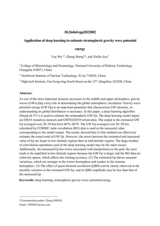
understanding its global distribution is necessary. In this paper, a deep learning algorithm
(DeepLab V3+) is used to estimate the stratospheric GW Ep. The deep learning model inputs
are ERA5 reanalysis datasets and GMTED2010 terrain data. The output is the estimated GW
Ep averaged over 2030 km from 60°
S60°
N. The GW Ep averaged over 20~30 km
calculated by COSMIC radio occultation (RO) data is used as the measured value
corresponding to the model output. The results showed that (1) this method can effectively
estimate the zonal trend of GW Ep. However, the errors between the estimated and measured
value of Ep are larger in low-latitude regions than in mid-latitude regions. The large number
of convolution operations used in the deep learning model may be the main reason.
Additionally, the measured Ep has errors associated with interpolation to the grid, the error
tends to be amplified in low-latitude regions because the GW Ep is larger and the RO data are
relatively sparse, which affects the training accuracy. (2) The estimated Ep shows seasonal
variations, which are stronger in the winter hemisphere and weaker in the summer
hemisphere. (3) The effect of quasi-biennial oscillation (QBO) can be clearly observed in the
monthly variation in the estimated GW Ep, and its QBO amplitude may be less than that of
the measured Ep.
Keywords: deep learning; stratospheric gravity wave; potential energy
*Corresponding author: Zheng SHENG
Email: 19994035@sina.com

1. Introduction
Atmospheric gravity waves (GWs) are mesoscale disturbances that exist in the global
atmosphere and have a global propagation effect (Alexander, 1998). GWs play a key role in
the coupling of the lower and upper atmosphere (Fritts and Alexander, 2003) and in the
dynamics and circulation of the middle atmosphere (John and Kumar, 2012). After GWs are
excited in the troposphere, the driving force generated by the upward propagation, saturation
and break-up process of GWs is an important source for the structure of the middle
atmosphere (Chen D et al., 2012, 2013). It is generally believed that GWs excited by
topography, convection and wind shear in the lower atmosphere will transport momentum
and energy to the middle atmosphere (Alexander, 1996) and interact with the background
atmosphere and other atmospheric waves. With the decrease in atmospheric density, the
amplitudes of GWs will increase when they propagate to the upper atmosphere after being
excited in the troposphere, and then they will reach an instability saturation condition.
Finally, GWs will break up and transfer their momentum and energy to the background
atmosphere and change the atmospheric background state.
In the study of GWs, it is a research hotspot to obtain the potential energy (Ep),
wavelength, propagation direction, momentum flux and other parameters of GWs from
sounding data (Xu XH et al., 2015). The data used to study GWs mainly come from
radiosonde (Yoshiki and Sato, 2000; Kramer et al., 2016), sounding rocket (Hamilton, 1991),
lidar (Zhao RC et al., 2016), and spaceborne equipment (Wang L and Alexander, 2010).
Although sounding rockets, radiosondes, radars, etc. have provided valuable measurement
data for the study of atmospheric GW activity, it is difficult to achieve a global distribution of
GWs by this equipment. Compared with data from other observation methods, satellite
observation data have a wider spatial range and can be used to study the large-scale or global
distribution of atmospheric GW parameters. Alexander et al. (2008) made a global analysis of
HIRDLS (High Resolution Dynamics Limb Sounder) temperature profile data to derive
properties of gravity waves. Meyer et al. (2018) compared temperature variances of AIRS
(Atmospheric InfraRed Sounder) and HIRDLS to evaluate the relationship of their
stratospheric gravity wave observations. Liu X et al. (2019) studied the seasonal and height
dependencies of the orographic primary and larger-scale secondary gravity waves using the
temperature profiles of SABER (Sounding of the Atmosphere using Broadband Emission
Radiometry).
Since the end of the 20th century, the method of measuring atmospheric parameters
by Global Navigation Satellite System (GNSS) radio occultation (RO) technology has been
widely used and many achievements have been made (Chen et al., 2018; Cheng N et al.,
2021). By measuring the bending angle and signal delay of the radio signal transmitted by the
satellite when the signal passes through the atmosphere, the atmospheric refractivity,
temperature, pressure, water vapor pressure and ionospheric electron density profiles can be
calculated (Luo J et al., 2018). GNSS RO has the advantages of high precision, high vertical
resolution, all-weather observation and global coverage (Bai WH et al., 2020). This
technology has become an important approach to global atmospheric measurement. In
investigations of GWs using GNSS RO data, Xu XH et al. (2018) determined the spatial and

temporal variability of global stratospheric GWs and the characteristics of GW activity
during sudden stratospheric warming (SSW) using COSMIC RO data.
In recent years, deep learning has played an important role in investigations of
weather and climate prediction (Rasp et al., 2018; Scher, 2018; Moraux et al., 2019).
However, there are still few studies using deep learning to estimate atmospheric GW
parameters. Only Matsuoka et al. (2020) used 29-year reanalysis datasets to estimate the flux
of GWs near the Hidaka Mountains in Japan by deep learning. Although reanalysis datasets
can cover the world horizontally and have high horizontal resolution, their vertical resolution
is generally low and cannot be used to obtain gravity wave potential energy (GW Ep).
Therefore, it is impossible to rely solely on reanalysis datasets to estimate GW Ep by deep
learning. The investigation of Matsuoka et al. (2020) innovatively applied deep learning to
estimate GW parameters, but due to the small region that was selected, it could not reflect the
spatial and temporal variability of global GW activities.
Taking ERA5 global reanalysis datasets and terrain data as input and taking the global
GW Ep calculated by the COSMIC RO data as the label, this study applies deep learning
(DeepLab V3+) to estimate the GW Ep averaged over 2030 km in the latitude range of
60°
S60°
N (as the output of the model). Additionally, this study verifies that GW Ep
estimated by the trained model has significant seasonal variation and quasi-biennial
oscillation.
Generally, COSMIC RO data can be used to study GW activities only after 2007,
while the global distribution of GW Ep before 2007 cannot be determined. The significance
of this study is to estimate the GW Ep in recent decades by using a large number of
reanalysis datasets to understand the long-term distribution of GWs in the middle and low
latitudes.
2. Datasets
2.1 Reanalysis Datasets
ERA5 is the fifth generation European Centre for Medium-Range Weather Forecasts
(ECMWF) reanalysis for the global climate and weather. The input data of the deep learning
model in this study are mainly the atmospheric parameters of ERA5 at certain pressure levels.
Since the excitation conditions of GWs mainly include terrain, wind shear, and deep
convection, the input parameters of ERA5 selected in this study include temperature, u-
component of wind (zonal wind), v-component of wind (meridional wind), vertical velocity
and relative humidity at 500, 700 and 850 hPa. To enable the deep learning model to learn the
quasi-biennial oscillation (QBO) characteristics of GWs, the input should include some
atmospheric parameters with QBO characteristics, so temperature and zonal wind at 50, 100
and 200 hPa are appended to the model input.
2.2 Terrain Data
Terrain is one of the most important reasons for the excitation of GWs, so terrain data
should also be used as the input data. The Global Multi-resolution Terrain Elevation Data
2010 (GMTED2010) is a notably enhanced global elevation model developed by the U.S.

Geological Survey (USGS) and the National Geospatial-Intelligence Agency (NGA). In this
study, its global mean elevation is input to the deep learning model.
2.3 COSMIC RO Data
The COSMIC mission is an Earth atmosphere detection system composed of a series
of low-orbit satellites. It is mainly applied in the study of weather forecasting, atmospheric
processes, climate monitoring, model verification, space weather, ionospheric research, etc.
The high accuracy and vertical resolution (~20 m in the L2 data) of COSMIC RO data enable
the calculation of the global GW Ep. This paper uses COSMIC RO data to calculate the GW
Ep averaged over 20~30 km as the measured values applied in the training process.
3. Method
For the sake of simplicity, in this paper the GW Ep calculated by COSMIC RO data is
called the measured value, and the GW Ep output by the deep learning model is called the
estimated value.
3.1 Calculation of GW Ep with COSMIC RO
The key to GW calculation is to extract the perturbation of the temperature profile
caused by GWs. This paper refers to the method developed by Wang L and Alexander (2009)
to obtain the temperature perturbation with COSMIC RO data and similar method has been
used in many related studies (Wang L and Alexander, 2010; Xu XH et al., 2015, 2018; Zeng
XY et al., 2017). The procedure is as follows:
(a) Interpolating. The cubic spline interpolation method is used to interpolate the
profile data over 8~38 km in altitude to a regular 200 m resolution.
(b) Eliminating abnormal profile data. There are still some abnormal temperature
profiles in the COSMIC L2 data (Figure 1a). To avoid the effects of these abnormal profiles
on the subsequent calculation of GW Ep, it is necessary to eliminate them. The method in
detail is as follows:
 Performing box-plot analysis on each interpolated profile at each level to provide a
reasonable temperature interval for each height (Figure 1b). Temperature values that
are not in the reasonable interval at each altitude level are regarded as the abnormal
values of the profiles.
 Counting the number of abnormal values in each profile. If the number of abnormal
values in a profile exceeds a certain threshold, this temperature profile is deemed to
be an abnormal temperature profile that needs to be eliminated. All temperature
profiles after eliminating abnormal data are shown in Figure 1c.

Figure 1. COSMIC RO temperature profiles on January 1, 2011 (UTC). (a) All unprocessed
temperature profiles (1305 profiles in total). (b) Box-plot analysis of each level. (c) All
temperature profiles after eliminating abnormal data (1094 profiles in total).
(c) Gridding of temperature data. A global grid is constructed at each level, and the
resolution of the region is 15°
×
10°which is sparse enough to obtaining the large-scale
background temperature. The mean of all temperature values in the grid is taken as the
temperature at the center point of the grid.
(d) Calculating large-scale waves. The S transform (Stockwell et al., 1996) is
performed to extract the large-scale temperature variation at each latitude. Temperature
variations with zonal wavenumbers between 0 and 6 can be regarded as large-scale waves,
which include planetary waves and Kelvin waves, while the residual term (i.e., waves with
zonal wavenumbers greater than 6) is considered to be mainly caused by GW activity (Jia Y
et al., 2015).
(e) Obtaining temperature perturbation. After interpolating the large-scale temperature
variation back to the position of the raw profiles as background temperature profiles (Figure
2a), temperature residuals can be obtained by subtracting background profiles from the
interpolated profiles of step (b). However the residuals still include some noise and need to
be filtered by a repeat S transform (Figure 2b).

Figure 2. A COSMIC RO temperature profile obtained on January 1, 2011 (UTC). (a) Raw
temperature profile and background temperature profile. (b) Temperature perturbation
profile.
After obtaining all temperature perturbation profiles, the GW Ep at each level can be
calculated by Eq. (1):
𝐸𝑝 =
1
2
(
𝑔
𝑁
)2
(
𝑇′
𝑇
̅
)2
(1)
where 𝑔 is the acceleration of gravity, 𝑇′
is the disturbance temperature, 𝑇
̅ is the
background temperature, and the Brunt-Vä
isä
läfrequency 𝑁 can be obtained from 𝑁2
in
Eq. (2):
𝑁2
=
𝑔
𝑇
̅
(
𝜕𝑇
̅
𝜕𝑧
+
𝑔
𝑐𝑝
) (2)
where 𝑧 is the altitude and 𝑐𝑝 is the isobaric specific heat.
Finally, constructing a global grid with a resolution of 1°
×
1°to interpolate the
scattered gravity wave potential energy data into regular grid data. The gridded global GW
Ep can be obtained (Figure 3).

Figure 3. Gridded GW Ep averaged over 2030 km on January 1, 2011 (UTC).
Due to the sparse distribution of COSMIC RO data in high latitudes (Figure 4a), the
gridded Ep may have null values in high-latitude regions. Additionally, with the gradual
reduction in the quantity of COSMIC-1 daily profiles after 2011 (Luo J et al., 2018) and
because the distribution of COSMIC-2 data after October 2019 is only between 60°
S and
60°
N (Figure 4b), to retain as much of the available data as possible, this study sets the target
region as 60°
S60°
N.

Figure 4. Distribution of COSMIC RO events on (a) January 1, 2011 (UTC) and (b) January
1, 2020 (UTC).
3.2 Dataset Construction and Augmentation
3.2.1 Dataset construction
It is generally accepted that the main excitation conditions of atmospheric GWs
include topography, deep convection, and wind shear (Fritts and Alexander, 2003). Among
these excitation mechanisms, topography is the more common sources of GWs (Zeng XY et
al., 2017), while in equatorial and low-latitude regions, GWs induced by convection are more
obvious (Vincent and Alexander, 2000). Because topographic GWs are mainly generated
around large terrains such as mountains, topographic data should be used as an input
parameter. The wind field can reflect the fluctuation of the atmosphere, and the
characteristics of the atmospheric fluctuation will be propagated upward after excitation of
GWs occurs in the troposphere, therefore, the wind field should be included as an input
parameter; Because strong convection is usually accompanied by high temperature and
humidity, temperature and humidity are also included as input parameters. However, the use
of only terrain, tropospheric temperature, humidity and wind fields as model inputs is not
sufficient to reflect the quasi-biennial variation characteristics of GW activity (this will be
illustrated in detail in the "results and discussion" section), therefore, it is necessary to add
the stratospheric temperature field and zonal wind with QBO characteristics as input. It is
worth mentioning that some studies have pointed out that there is a strong correspondence
between stratospheric GW Ep and zonal wind (Zeng XY et al., 2017; Xu XH et al., 2018). In
Figure5, taking the zero-wind speed line (white solid line) as the boundary, the potential
energy of the east wind area in the middle latitude surrounded by the zero-wind speed line is
smaller, while the potential energy of the west wind area is larger. Below the height of 20
km, the upload of gravity wave activity is significantly affected by the zero-wind layer. In
Figure6, the maximum Ep in low latitudes appears near the zero-wind speed line. The blank
area regions in Figure5 and 6 represent that Ep in these regions is greater than the maximum
(4 J/kg) of the colorbar. The wind field data in Figure5 and Figure 6 is from ERA5.

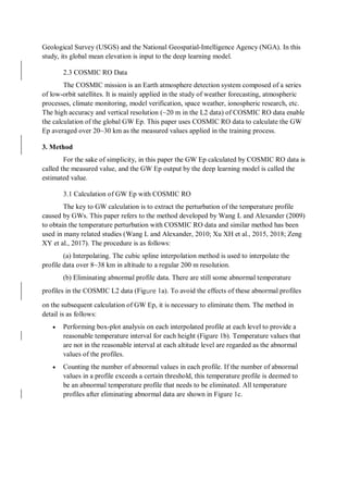
Figure 5. The monthly average variation of GW Ep and zonal wind at each altitude in the
latitude range of 30°
N40°
N from 2007 to 2014 (the heat map is the GW Ep, the isoline is
the zonal wind, the negative zonal wind values [black dotted lines] represent east wind, and
the positive values (red solid lines] represent west wind).
Figure 6. Same as Figure 5, but for 10°
S10°
N.
The input data of the deep learning model have 22 layers, and the region of each layer
is 60°
S60°
N. A downsampling operation is performed to achieve a resolution of 1°
×
1°
,
which is the same as the resolution of the gridded GW Ep. All input layers are shown in
Table 1. The output of the model is the GW Ep grid data within the area of 60°
S60°
N.
Table 1. Input dataset of the deep learning model.
Layer Parameter name
Pressure levels
(hPa)
Resolution Latitude range
1 Terrain / 1°
×
1° 60°
S60°
N
24 Relative humidity 500, 700, 850 1°
×
1° 60°
S60°
N
57 Temperature 500, 700, 850 1°
×
1° 60°
S60°
N
810 Zonal wind 500, 700, 850 1°
×
1° 60°
S60°
N
1113 Meridional wind 500, 700, 850 1°
×
1° 60°
S60°
N
1416 Vertical velocity 500, 700, 850 1°
×
1° 60°
S60°
N
1719 Temperature 50, 100, 200 1°
×
1° 60°
S60°
N
2022 Zonal wind 50, 100, 200 1°
×
1° 60°
S60°
N
To accelerate the convergence of the model, it is necessary to normalize the data of
each layer. For the input/output layer 𝐴, its maximum and minimum values, Max and Min,

in the global range over the years examined can be determined, and the normalization
operation for 𝐴 can be expressed as [𝐴 − (Min − 𝜀1)]/[(Max + 𝜀2) − (Min − 𝜀1)], where
(Min − 𝜀1) and (Max + 𝜀2) represent an appropriate expansion of the value range to ensure
that the normalization operation always has an input/output data value between 0 and 1 when
new data are input in the model.
To verify the seasonal variation in the estimated Ep, datasets from three years (June
2009 to May 2010, June 2010 to May 2011, and June 2011 to May 2012) were used as test
sets to evaluate three models separately. For each model, 5% of the data outside the test set
were randomly selected as the validation set and the other data were used as the training set.
The date range of the training set, validation set and test set of the three models are shown in
Table 2. This study uses three models is to verify that the seasonality of GW Ep is not the
result typical of other years, because the intensity of GW Ep is different in these three years.
Table 2. Date range of the training set, validation set and test set.
Model Training and validation set Test set
Model 1
2006.122009.05
&
2010.062020.12
2009.062010.05
Model 2
2006.122010.05
&
2011.062020.12
2010.062011.05
Model 3
2006.122011.05
&
2012.06~2020.12
2011.062012.05
3.2.2 Dataset augmentation
Since the calculation of the measured values of GW Ep requires all the temperature
profile data from each day, only one global distribution of GW Ep can be obtained for each
day. The time span of COSMIC RO data in this paper is from January 2007 to December
2020, and the quantities of daily profiles on many days are not enough to calculate the global
distribution of GW Ep, so there are only approximately 3300 valid days, which is far from
enough for deep learning. Hence, it is necessary to augment the dataset.
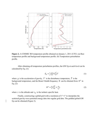
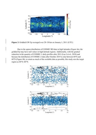
This study develops a "cut-swap" dataset augmentation method for global
meteorological data. Taking terrain data as an example, the specific steps for dataset
augmentation are as follows:
(a) Select an integer longitude within the longitude range of 180°
W180°
E and cut
the dataset along that longitude (Figure 7a).
(b) Swap the left and right parts of the split dataset and then re-splice them together
(Figure 7b).

(c) Repeat the above processes 14 times to expand the sample size to approximately
50000, which is 15 times the original amount.
Figure 7. Steps of dataset augmentation. (a) Cut the dataset along a random longitude. (b)
Swap the split dataset and re-splice them together.
The input layers (terrain and reanalysis data) and the output layer (measured Ep) of
the training set are processed simultaneously using the dataset augmentation method. Dataset
augmentation can not only greatly increase the quantity of training samples but also enable
the deep learning model to learn the internal relationship between terrain and GW activities.
Without dataset augmentation, the terrain data input to the deep learning model is invariant.
Such constant terrain data are not helpful to the gradient descent of the deep learning model’s
parameters, and cannot reflect the effect of terrain on GW activity.
3.2.3 Deep learning model
DeepLab is a successful deep learning model in the field of semantic segmentation
and is mostly used for image classification (Chen et al., 2018; Ren YY et al., 2020). In this
study, the DeepLab V3+ deep learning model is used to estimate stratospheric GW Ep, and
the ideal results are also obtained. DeepLab V3+ is mainly composed of an encoder and a
decoder (the model structure is shown in Figure 8). The Adam optimizer and mean square
error (MSE) loss function are used to train the model.

Figure 8. The model structure of DeepLab V3+.
4 Results and Discussion
4.1 Training Results
As illustrated by Model 2, after 25 epochs of training, the losses of the training set
and validation set are reduced to 0.00024 and 0.0003, respectively (Figure 9). Since the
output GW Ep of the model is normalized (the value range of the GW Ep averaged over
2030 km is 010 J/kg), the calculation of the loss function uses the normalized values of Ep
instead of the original values. The MSE loss function can be expressed as Eq. (3).
𝑀𝑆𝐸 =
1
𝑚∗𝑛
∑ ∑ (𝑇𝑖𝑗 − 𝑃𝑖𝑗)2
𝑛
𝑗=1
𝑚
𝑖=1 (3)
where 𝑇𝑖𝑗 is the normalized measured value of GW Ep in the i-th row and j-th column, 𝑃𝑖𝑗 is
the normalized estimated value of GW Ep in the i-th row and j-th column, and m and n are
the rows and columns of Ep grid data, respectively. In this paper the values of m and n are
120 and 360. In Figure 9, the losses of the validation set and training set are similar, which
means that the model does not overfit. The final loss of test set is 0.0009.

Figure 9. Losses of the training set and validation set.
Figure 10 shows the estimated results of the GW Ep averaged over 20~30 km from
the 8th to the 11th of June 2010 by using the trained DeepLab V3+ model (Model 2). Taking
Fig. 10b as an example, some high-value areas in low latitudes and low-value areas in mid-
latitudes can be found in both the measured and estimated GW Ep (shown as the marked area
in Figure 10b). In the four examples selected in Fig. 10, there is stronger GW Ep in the low
latitudes, so the meridional mean GW Ep (both measured and estimated Ep) of 20°
S20°
N is
calculated. The third graph of each panel in Figure 10 also compares the measured Ep with
the estimated Ep of 20°
S20°
N, and the longitudes of the extreme points of the measured and
estimated Ep are almost the same (blue lines in Figure10), which means that the zonal
variation of the estimated GW Ep is generally consistent with that of the measured values.
(a) 2010-06-08 (b) 2010-06-09
(c) 2010-06-10 (d) 2010-06-11

Figure 10. GW Ep averaged over 2030 km from the 8th to the 11th of June 2010 (the three
graphs of each panel from top to bottom indicate the measured GW Ep, estimated GW Ep
and the meridional mean GW Ep of 20°
S20°
N, respectively).
However, Figure 10, especially Figure10d, also shows that the error between the
estimated Ep and the measured Ep in the low-latitude regions is larger than that in the mid-
latitude regions. The estimated Ep is weaker than the measured Ep, and a larger Ep results in
a larger regional error. The five main reasons for this finding are listed below:
(a) The DeepLab model uses many convolution operations, which causes the error of
the mean Ep within a certain range to be smaller and the error of a single grid point to be
larger. As shown in Figure 10a-c, the estimated Ep is smaller than the measured Ep in the
area where the Ep is larger, while the meridional mean values between 20°
S~20°
N of the
measured and estimated Ep are almost the same.
(b) Due to the low horizontal resolution of COSMIC RO data, large errors will
inevitably occur when GW Ep calculated by temperature profiles is interpolated to a global
grid with a 1°
×
1°horizontal resolution.
(c) GW Ep in the low-latitude regions is greater than that in the mid-latitudes, and the
RO data in the equatorial and polar regions are sparser than those in the mid-latitude regions
(Wang L and Alexander, 2010), so the interpolation errors in low-latitude regions tend to be
amplified.
(d) To minimize the overall error in the training process, the deep learning model
learns the deep correlation between the input data and Ep, so the estimated value may not
perfectly match the measured GW Ep in some cases. However, the overall error is lower on
long time scales (such as the seasonal mean GW Ep), which will be illustrated in the next
section.
(e) Because data with larger Ep account for a small proportion of the data, most of the
data used for model training have smaller Ep; therefore, the estimated value of the area with
larger Ep will be inaccurate.
4.2 Seasonal Variation in GW Ep
Due to the low horizontal resolution of daily RO data, the calculated daily global
distribution of GW Ep is not significantly representative. Much of the related studies on the
calculation of GW Ep with COSMIC RO data focus on the monthly or seasonal trend of Ep
(Xu XH et al., 2018; Yu DC et al., 2019).
To verify whether the model can accurately describe the seasonal variation in
stratospheric GW Ep, this study used the trained model to estimate GW Ep with the test set.
The measured and estimated values of GW Ep were seasonally averaged separately. Each
model uses a whole year of data as the test set, which can be divided into four seasons: JJA
(Jun-Jul-Aug), SON (Sep-Oct-Nov), DJF (Dec-Jan-Feb) and MAM (Mar-Apr-May). The
seasonal means of the measured and estimated GW Ep of the three models are shown in
Figure 11-13.

(a) JJA (b) SON
(c) DJF (d) MAM
Figure 11. Seasonal means of GW Ep over 2030 km from Jun 2009 to May 2010 by Model
1 (the three graphs of each panel from top to bottom indicate the measured GW Ep, estimated
GW Ep and error between the measured and estimated Ep, respectively).

(a) JJA (b) SON
(c) DJF (d) MAM
Figure 12. Same as Figure 11, but for seasonal means of GW Ep over 20~30 km from Jun
2010 to May 2011 by Model 2.

(a) JJA (b) SON
(c) DJF (d) MAM
Figure 13. Same as Fig.ure11, but for seasonal means of GW Ep over 20~30 km from Jun
2011 to May 2012 by Model 3.
The RMSEs (root mean square errors) between the seasonal means of the measured
and estimated GW Ep in JJA, SON, DJF and MAM are shown in Table 3.
Table 3. RMSEs between the seasonal means of the measured and estimated GW Ep.
Model
RMSE (J/kg)
JJA SON DJF MAM
Model 1 0.089 0.063 0.193 0.085
Model 2 0.2 0.06 0.074 0.062
Model 3 0.074 0.068 0.1 0.06

Xu XH et al. (2018) pointed out that GW Ep in the winter hemisphere is higher than
that in the summer hemisphere in extratropical regions, which might be attributable to the
influences of orography and zonal wind. Additionally, the GW Ep in equatorial regions is
higher than that in extratropical regions. These conclusions can be confirmed by both the
measured and estimated values of GW Ep in JJA and DJF of Figure 11-13. The Southern
Hemisphere is the winter hemisphere in Figure 12a, and the GW Ep in the mid-latitude
regions of the Southern Hemisphere is significantly higher than that in the mid-latitude
regions of the Northern Hemisphere, while Figure 12c shows the opposite phenomenon. In
terms of seasonal distribution characteristics of GW Ep, there are also some research results
of SABER/TIMED satellites (Zhang Y et al., 2012). Compare with the seasonal distribution
of Ep in the study of Zhang Y et al. (2012), our research results are slightly different, e.g., the
Ep in mid latitude at winter in their study is stronger than that in this study. This maybe
because of the different data source and data processing method.
In addition, in the two seasons of JJA and SON, GW Ep is stronger near 80°
W in the
southern hemisphere, and it extends eastward. This is due to the GW activity caused by the
topography of the Andes Mountains in South America. Figure 11-13 show that these three
models all can accurately estimate the GW Ep in this area, which also demonstrates that the
deep learning model used in this study can learn the influence of terrain on GW activity.
Figure 11~13 also show that the GW activity of JJA in 2010 was significantly
stronger than that in 2009 and 2011, and the estimated model results also correctly reflect this
intensity variation. Additionally, the RMSEs between the seasonal average values of the
measured and estimated Ep are small, which indicates that the method used in this paper can
accurately reflect the seasonal variation characteristics of GW activity.
4.3 Quasi-biennial Oscillation of GW Ep
QBO usually refers to the phenomenon that the tropical lower stratospheric zonal
wind alternates between easterly and westerly winds. This phenomenon also occurs in the
stratospheric GW Ep in low-latitude regions (Xu XH et al., 2018). The QBO of Ep calculated
by COSMIC RO data from 2007.01 to 2013.12 is shown in Figure 14. A 13-month moving
average is performed to remove the annual change, so that the QBO results will be clearer.

Figure 14. Measured Ep from 2007.01 to 2013.12 calculated by COSMIC RO data. (a)
Variation in zonal mean GW Ep with time. (b) Variation in the mean GW Ep within the
latitude range of 20°
S20°
N with time. (c) The mean GW Ep within the latitude range of
20°
S20°
N after 13-month moving average processing.
In this study, to enable the deep learning model to learn the QBO characteristics, the
temperature and zonal wind fields at 50, 100 and 200 hPa of the ERA5 reanalysis dataset
need to be added to the input data (the temperature field and zonal wind field in the
stratosphere have significant QBO characteristics).
As illustrated by the example of Model 2, to verify whether the model can describe
the QBO effect of stratospheric GW Ep in low-latitude regions, this study uses the deep
learning model to estimate the GW Ep from 2000 to 2006 (since the data after 2007 are
involved in the training of the model, even if the estimated Ep after 2007 exhibits QBO
characteristics, it does not indicate that the model actually learns QBO characteristics).
Figure 15 shows the estimated Ep from 2000.01 to 2006.12 output by the deep learning
model.

Figure 15. Estimated Ep from 2000.01 to 2006.12 according to Model 2. (a) Variation in
zonal mean GW Ep over time. (b) Variation in the mean GW Ep within the latitude range of
20°
S20°
N over time. (c) The mean GW Ep within the latitude range of 20°
S20°
N after 13-
month moving average processing.
As shown in Figure 14, the measured Ep from 2007 to 2013 shows a significant QBO
effect in low-latitude regions, and strong years and weak years of GW Ep alternately appear
in low-latitude regions. Additionally, QBO occurs in the estimated Ep from 2000 to 2006, as
shown in Figure 15. Although the model is unable to obtain measured values of GW Ep from
2000 to 2006 for comparison, it appears that the trained model has learned the QBO
characteristics of GWs. Although the model can predict the QBO characteristic of Ep, its
QBO amplitude may be less than that of the measured Ep (Figure14c and 15c), which means
that the model cannot perfectly estimate the long-term variation of GW Ep.
The QBO characteristics of Ep can be learned by the model mainly because the
stratospheric temperature and zonal wind in the input parameters of the model also have
QBO characteristics. When the stratospheric temperature and zonal wind (layers 17~22) in
the input parameters are omitted, the resulting estimated average GW Ep of 20-30 km from
2000.01 to 2006.12 is shown in Figure 16, and there is no obvious quasi-biennial variation in
the low-latitude region.

Figure 16. Estimated Ep from 2000.01 to 2006.12 by the DeepLab V3+ model without
stratospheric temperature and zonal wind. (a) Variation in zonal mean GW Ep with time. (b)
Variation in the mean GW Ep within the latitude range of 20°
S20°
N with time. (c) The
mean GW Ep within the latitude range of 20°
S20°
N after 13-month moving average
processing.
5 Conclusions
In this paper, a DeepLab V3+ deep learning model is applied to estimate stratospheric
GW potential energy. Using the trained deep learning model, direct mapping from the
reanalysis data at 50, 100, 200, 500, 700 and 850 hPa and terrain data to the GW Ep averaged
over 2030 km can be realized.
Since the sources of GWs are mainly terrain, wind shear and deep convection,
temperature, wind field, and relative humidity in the troposphere (500, 700, 850 hPa) are
considered as the input of the model. To reflect the QBO characteristics of GWs, temperature
and zonal wind fields at 50, 100 and 200 hPa need to be added to the input data. A “cut-
swap” approach is applied to augment the dataset. Additionally, this augmentation method
can make the input terrain data changeable, which ma2y help the model learn the relationship
between terrain and GW activities.
The results show the following:
(1) This deep learning method can effectively estimate the zonal trend of the GW Ep
averaged over 20~30 km. However, the errors in low-latitude regions are larger than those in
mid-latitude regions. The main reason is that the large number of convolution operations used
in the deep learning model causes the error of the mean Ep within a certain range to decrease
and the error of single grid point to increase. In addition, the horizontal resolution of

COSMIC RO data is low, and the RO data at low latitudes are sparser than those at middle
latitudes, so the interpolation process of constructing the grid data of measured Ep tends to
cause larger errors at low latitudes. These errors also have a great impact on the accuracy of
model training.
(2) The estimated results of the model show significant seasonal variations in which
GW activity is strong in winter and weak in summer. The seasonal variation reflected in the
estimated Ep is consistent with that reflected in the measured Ep calculated by COSMIC RO
temperature profiles.
(3) This model can learn the QBO characteristics of GWs. With the input of
reanalysis data from 2000 to 2006 and terrain data, the average GW Ep at heights of 2030
km during these seven years estimated by the deep learning model shows significant QBO
characteristics.
The significance of this study is the verification of the feasibility of the deep learning
method to estimate GW Ep. Abundant reanalysis data can be used to estimate stratospheric
GW Ep in recent decades so that the long-term variation in stratospheric GWs in mid- and
low-latitude regions can be determined. Additionally, for future studies, numerical prediction
can also be considered as inputs of the deep learning model to realize the prediction of GW
Ep.
Acknowledgments
We would like to thank all the editors and the anonymous reviewers for their help in the
development and improvement of this paper. The COSMIC RO data was downloaded from
https://cdaac-www.cosmic.ucar.edu/. The GMTED2010 terrain data was downloaded from
https://www.usgs.gov/core-science-systems/eros/coastal-changes-and-impacts/gmted2010.
The ERA5 hourly data on pressure levels was downloaded from
https://cds.climate.copernicus.eu/cdsapp#!/dataset/reanalysis-era5-pressure-levels.
References
Alexander, M. J. (1996). A simulated spectrum of convectively generated gravity waves:
propagation from the tropopause to the mesopause and effects on the middle atmosphere. J.
Geophys. Res.: Atmos., 101(D1), 1571-1588. https://doi.org/10.1029/95jd02046
Alexander, M. J. (1998). Interpretations of observed climatological patterns in stratospheric
gravity wave variance. J. Geophys. Res.: Atmos., 103(D8), 8627-8640.
https://doi.org/10.1029/97JD03325
Alexander, M. J., Gille, J., Cavanaugh, C., Coffey, M., Craig, C., Eden, T., Francis, G.,
Halvorson, C., Hannigan, J., … Dean, V. (2008). Global estimates of gravity wave
momentum flux from High Resolution Dynamics Limb Sounder observations. J. Geophys.
Res.: Atmos., 113(D15), D15S18. https://doi.org/10.1029/2007JD008807
Bai, W. H., Deng, N., Sun, Y. Q., Du, Q. F., Xia, J. M., Wang, X. Y., Meng, X. G., Zhao, D.
Y., Liu, C. L., … Liu, X. X. (2020). Applications of GNSS-RO to numerical weather
prediction and tropical cyclone forecast. Atmosphere, 11(11), 1204.
https://doi.org/10.3390/atmos11111204

Chen, D., Chen, Z. Y., and Lü
, D. R. (2012). Simulation of the stratospheric gravity waves
generated by the Typhoon Matsa in 2005. Sci. China Earth Sci., 55(4), 602-610.
https://doi.org/10.1007/s11430-011-4303-1
Chen, D., Chen, Z. Y., and Lü
, D. R. (2013). Spatiotemporal spectrum and momentum flux
of the stratospheric gravity waves generated by a typhoon. Sci. China Earth Sci., 56(1), 54-
62. https://doi.org/10.1007/s11430-012-4502-4
Chen, L. C., Papandreou, G., Kokkinos, I., Murphy, K., and Yuille, A. L. (2018). DeepLab:
semantic image segmentation with deep convolutional nets, Atrous convolution, and fully
connected CRFs. IEEE Trans. Pattern Anal. Mach. Intell., 40(4), 834-848.
https://doi.org/10.1109/TPAMI.2017.2699184
Chen, Z. P., Li, J. C., Luo, J., and Cao, X. Y. (2018). A new strategy for extracting ENSO
related signals in the troposphere and lower stratosphere from GNSS RO specific humidity
observations. Remote Sens., 10(4), 503. https://doi.org/10.3390/rs10040503
Cheng, N., Song, S. L., Jiao, G. Q., Jin, X. L., and Li, W. (2021). Global monitoring of
geomagnetic storm-induced ionosphere anomalies using 3-D ionospheric modeling with
multi-GNSS and COSMIC measurements. Radio Sci., 56(2), e2020RS007074.
https://doi.org/10.1029/2020RS007074
Fritts, D. C., and Alexander, M. J. (2003). Gravity wave dynamics and effects in the middle
atmosphere. Rev. Geophys., 41(1), 3-1-3-64. https://doi.org/10.1029/2001RG000106
Hamilton, K. (1991). Climatological statistics of stratospheric inertia-gravity waves deduced
from historical rocketsonde wind and temperature data. J. Geophys. Res.: Atmos., 96(D11),
20831-20839. https://doi.org/10.1029/91JD02188
Jia, Y., Zhang, S. D., Yi, F., Huang, C. M., Huang, K. M., Gan, Q., and Gong, Y. (2015).
Observations of gravity wave activity during stratospheric sudden warmings in the Northern
Hemisphere. Sci. China Technol. Sci., 58(6), 951-960. https://doi.org/10.1007/s11431-015-
5806-3
John, S. R., and Kumar, K. K. (2012). TIMED/SABER observations of global gravity wave
climatology and their interannual variability from stratosphere to mesosphere lower
thermosphere. Climate Dyn., 39(6), 1489-1505. https://doi.org/10.1007/s00382-012-1329-9
Kramer, R., Wü
st, S., and Bittner, M. (2016). Investigation of gravity wave activity based on
operational radiosonde data from 13 years (1997-2009): climatology and possible induced
variability. J. Atmos. Solar-Terr. Phys., 140, 23-33.
https://doi.org/10.1016/j.jastp.2016.01.014
Liu, X., Xu, J. Y., Yue, J., Vadas, S. L., and Becker, E. (2019). Orographic primary and
secondary gravity waves in the middle atmosphere from 16-year SABER observations.
Geophys. Res. Lett., 46(8), 4512-4522. https://doi.org/10.1029/2019gl082256
Luo, J., Chen, Z. P., and Xu, X. H. (2018). Specific humidity response in the troposphere and
lower stratosphere to ONI revealed by COSMIC observations. Chin. J. Geophys. (in
Chinese), 61(2), 466-476. https://doi.org/10.6038/cjg2018L0201

Matsuoka, D., Watanabe, S., Sato, K., Kawazoe, S., Yu, W., and Easterbrook, S. (2020).
Application of deep learning to estimate atmospheric gravity wave parameters in reanalysis
data sets. Geophys. Res. Lett., 47(19), e2020GL089436.
https://doi.org/10.1029/2020GL089436
Meyer, C. I., Ern, M., Hoffmann, L., Trinh, Q. T., and Alexander, M. J. (2018).
Intercomparison of AIRS and HIRDLS stratospheric gravity wave observations. Atmos.
Meas. Tech., 11(1), 215-232. https://doi.org/10.5194/amt-11-215-2018
Moraux, A., Dewitte, S., Cornelis, B., and Munteanu, A. (2019). Deep learning for
precipitation estimation from satellite and rain gauges measurements. Remote Sens., 11(21),
2463. https://doi.org/10.3390/rs11212463
Rasp, S., Pritchard, M. S., and Gentine, P. (2018). Deep learning to represent subgrid
processes in climate models. Proc. Natl. Acad. Sci. USA, 115(39), 9684-9689.
https://doi.org/10.1073/pnas.1810286115
Ren, Y. Y., Zhang, X. F., Ma, Y. J., Yang, Q. Y., Wang, C. J., Liu, H. L., and Qi, Q. (2020).
Full convolutional neural network based on multi-scale feature fusion for the class imbalance
remote sensing image classification. Remote Sens., 12(21), 3547.
https://doi.org/10.3390/rs12213547
Scher, S. (2018). Toward data-driven weather and climate forecasting: approximating a
simple general circulation model with deep learning. Geophys. Res. Lett., 45(22), 12616-
12622. https://doi.org/10.1029/2018gl080704
Song, Y. L. Z., and Huang, K. M. (2020). A radiosonde observation study of inertia gravity
waves over the high latitudes. J. Wuhan Univ. (Nat. Sci. Ed.) (in Chinese), 66(6), 541-551.
https://doi.org/10.14188/j.1671-8836.2020.0028
Stockwell, R. G., Mansinha, L., and Lowe, R. P. (1996). Localization of the complex
spectrum: the S transform. IEEE Trans. Signal Process., 44(4), 998-1001.
https://doi.org/10.1109/78.492555
Vincent, R. A., and Alexander, M. J. (2000). Gravity waves in the tropical lower
stratosphere: an observational study of seasonal and interannual variability. J. Geophys. Res.:
Atmos., 105(D14), 17971-17982. https://doi.org/10.1029/2000JD900196
Wang, L., and Alexander, M. J. (2009). Gravity wave activity during stratospheric sudden
warmings in the 2007-2008 Northern Hemisphere winter. J. Geophys. Res.: Atmos.,
114(D18), D18108. https://doi.org/10.1029/2009JD011867
Wang, L., and Alexander, M. J. (2010). Global estimates of gravity wave parameters from
GPS radio occultation temperature data. J. Geophys. Res.: Atmos., 115(D21), D21122.
https://doi.org/10.1029/2010JD013860
Xu, X. H., Guo, J. C., and Luo, J. (2015). Analysis of the global distribution of the
atmospheric gravity wave parameters using COSMIC radio occultation data. Geomat. Inf.
Sci. Wuhan Univ. (in Chinese), 40(11), 1493-1498.
https://doi.org/10.13203/j.whugis20130587

Xu, X. H., Yu, D. C., and Luo, J. (2018). The spatial and temporal variability of global
stratospheric gravity waves and their activity during sudden stratospheric warming revealed
by COSMIC measurements. Adv. Atmos. Sci., 35(12), 1533-1546.
https://doi.org/10.1007/s00376-018-5053-1
Yoshiki, M., and Sato, K. (2000). A statistical study of gravity waves in the polar regions
based on operational radiosonde data. J. Geophys. Res.: Atmos., 105(D14), 17995-18011.
https://doi.org/10.1029/2000jd900204
Yu, D. C., Xu, X. H., Luo, J., and Li, J. (2019). On the relationship between gravity waves
and tropopause height and temperature over the globe revealed by COSMIC radio occultation
measurements. Atmosphere, 10(2), 75. https://doi.org/10.3390/atmos10020075
Zeng, X. Y., Xue, X. H., and Dou, X. K., Liang, C., and Jia, M. J. (2017). COSMIC GPS
observations of topographic gravity waves in the stratosphere around the Tibetan Plateau. Sci.
China Earth Sci., 60(1), 188-197. https://doi.org/10.1007/s11430-016-0065-6
Zhang, Y., Xiong, J., Liu, L., and Wan, W. (2012). A global morphology of gravity wave
activity in the stratosphere revealed by the 8-year SABER/TIMED data. J. Geophys. Res.:
Atmos., 117(D21), D21101. https://doi.org/10.1029/2012jd017676
Zhao, R. C., Dou, X. K., Sun, D. S., Xue, X. H., Zheng, J., Han, Y. L., Chen, T. D., Wang, G.
C., and Zhou, Y. J. (2016). Gravity waves observation of wind field in stratosphere based on
a Rayleigh Doppler lidar. Opt. Express, 24(6), A581-A591.
https://doi.org/10.1364/OE.24.00A581

Application+of+deep+learning+to+estimate+stratospheric+gravity+wave+potential+energy.pdf

More Related Content

Recently uploaded

Featured

Application+of+deep+learning+to+estimate+stratospheric+gravity+wave+potential+energy.pdf