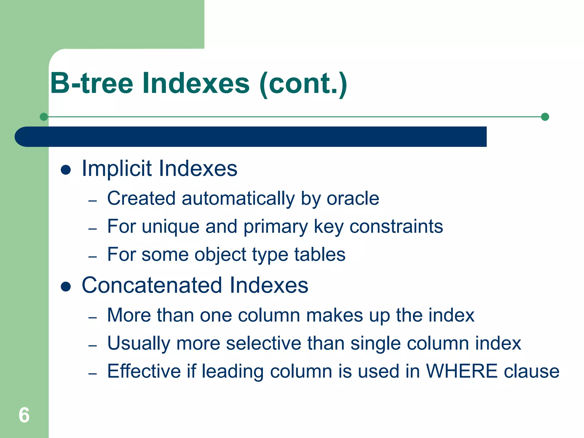
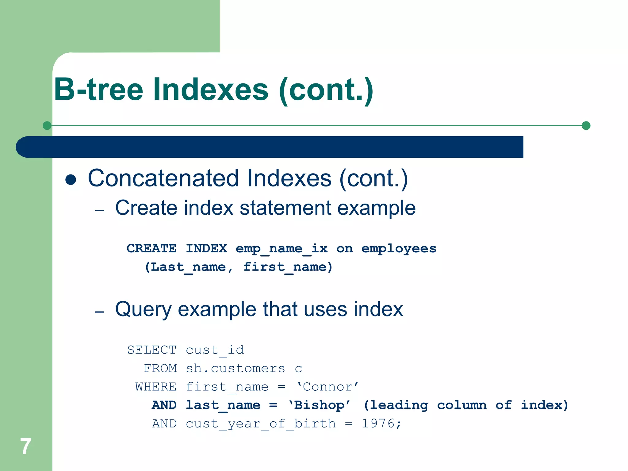
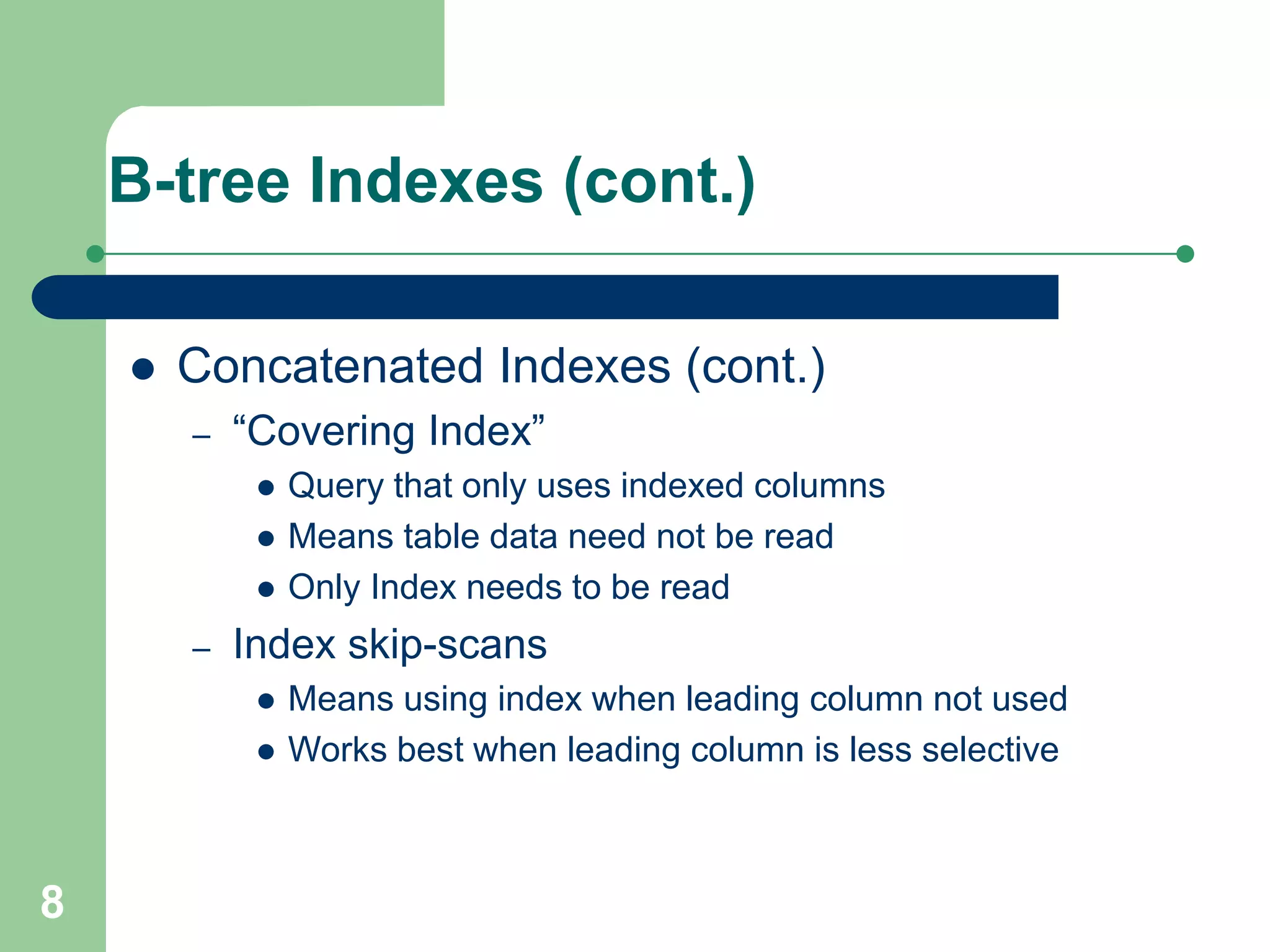
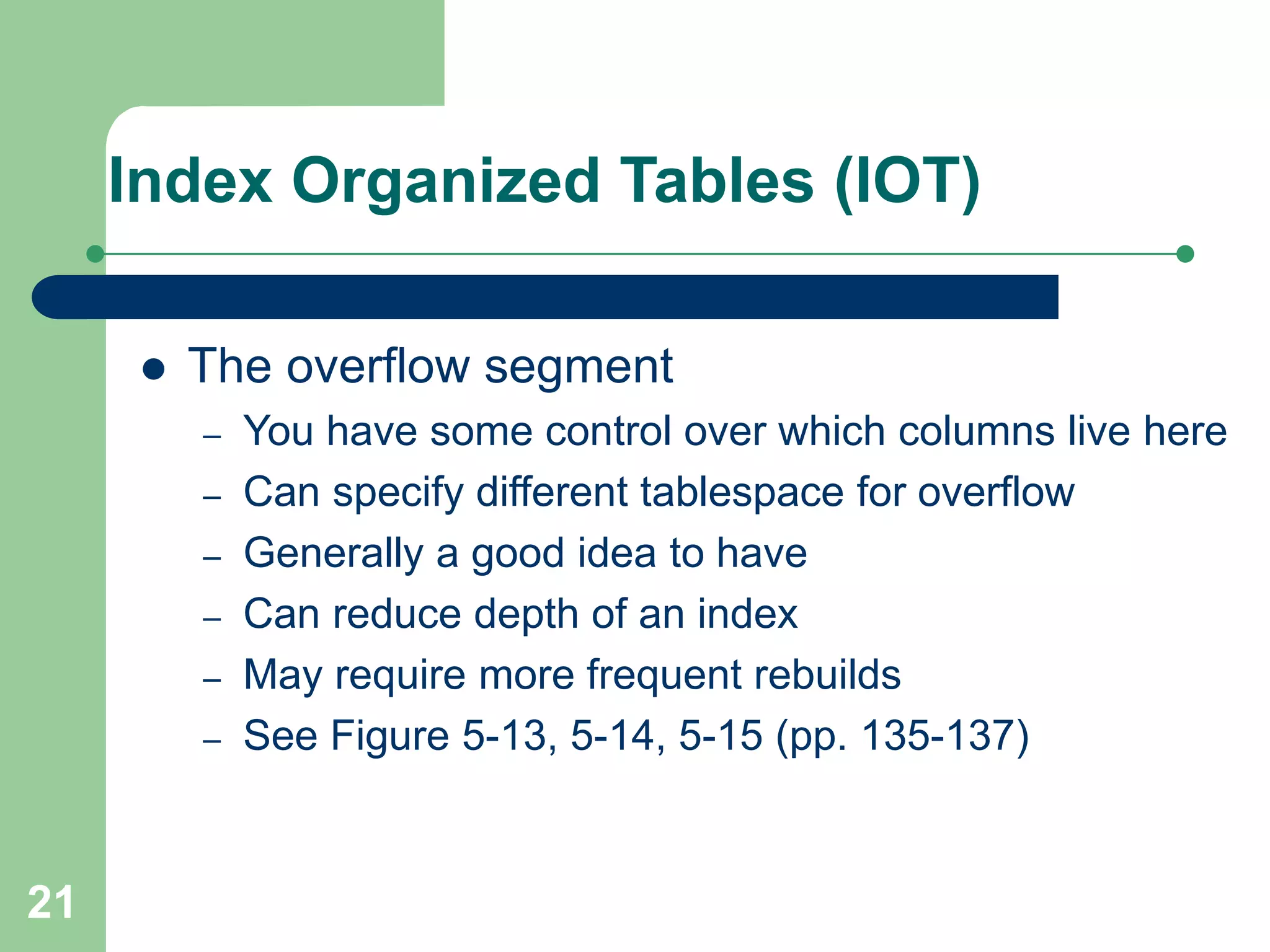
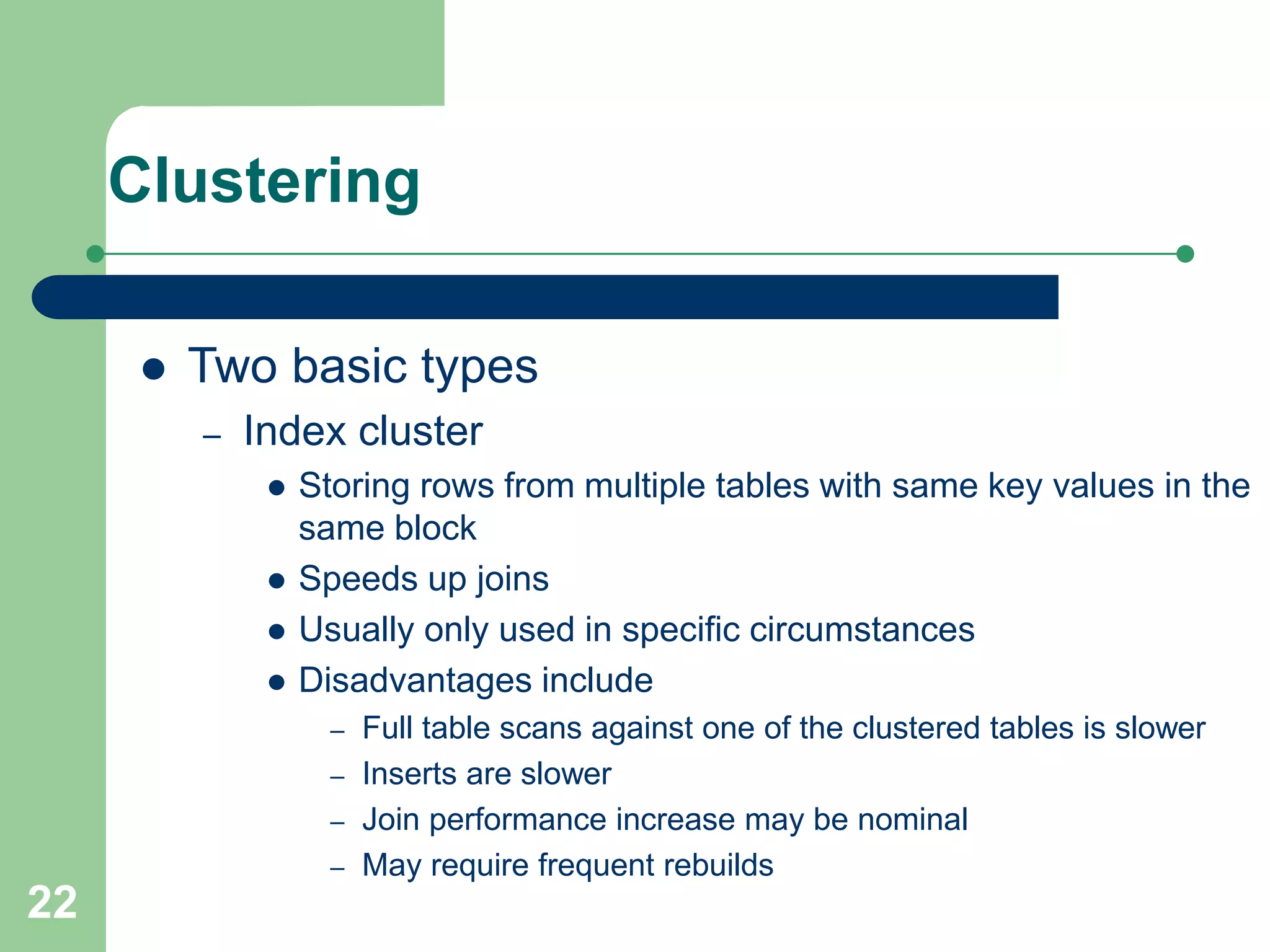
1
Chapter 5
Index and Clustering
2
Overview of Indexes and Clustering
 B-tree indexes
 Bitmap indexes (and bitmap join indexes)
 Index-organized tables (IOT)
 Hash Clusters
 Index Cluster
 Nested Tables
3
B-tree Indexes
 “Balanced tree” – has hierarchical tree
structure
– Header block
 Contains pointers to “Branch blocks” for given value sets
– Branch blocks
 Contains pointers to other branch blocks, or
 Contains pointers to “Leaf Blocks”
– Leaf Blocks
 Contains list of key values and pointers (ROWIDS) to
actual table row data
 See figures 5-1 (p. 112), 5-2 (p. 113)
4
B-tree Indexes (cont.)
 Can provide efficient query performance
– Header, branch blocks often in memory
– Reading leafs blocks to retrieve data requires often
few I/O’s
– Goal is to keep “balanced” tree
 Maintenance can be expensive
 Index splits can occur
– Reduces performances and increases I/O
– Requires rebuild to repair
5
B-tree Indexes (cont.)
 Index selectivity
– Is a measure of usefulness of an index
– Selective for columns with large number of unique
values
– More efficient than non-selective indexes because
they point to more specific values
 Unique Indexes
– No duplicate values allowed
– Very selective by nature
6
B-tree Indexes (cont.)
 Implicit Indexes
– Created automatically by oracle
– For unique and primary key constraints
– For some object type tables
 Concatenated Indexes
– More than one column makes up the index
– Usually more selective than single column index
– Effective if leading column is used in WHERE clause
7
B-tree Indexes (cont.)
 Concatenated Indexes (cont.)
– Create index statement example
CREATE INDEX emp_name_ix on employees
(Last_name, first_name)
– Query example that uses index
SELECT cust_id
FROM sh.customers c
WHERE first_name = ‘Connor’
AND last_name = ‘Bishop’ (leading column of index)
AND cust_year_of_birth = 1976;
8
B-tree Indexes (cont.)
 Concatenated Indexes (cont.)
– “Covering Index”
 Query that only uses indexed columns
 Means table data need not be read
 Only Index needs to be read
– Index skip-scans
 Means using index when leading column not used
 Works best when leading column is less selective
9
B-tree Indexes (cont.)
 Guidelines for use of concatenated indexes
– Create if WHERE clause needs these columns together
– Analyze which column is best suited to be the leading column
– The more selective a column is, the better it is as the leading
column
 Isn’t true if wanting to use only non-leading column
 Keep in mind Index skip-scan performs less than a normal range
scan (i.e. try to use leading column)
– Supports queries that doesn’t use all the columns of the index
in the WHERE clause (e.g. if only using the leading column)
10
B-tree Indexes (cont.)
 Index merges
– Performed by Oracle if more than one column in the
WHERE clause
– Is an alternative to a concatenated index if individual
indexes exist on columns in WHERE clause
– Merges values for the values of each column
– Generally less efficient than concatenated index
– If seen in EXPLAIN PLAN consider creating
concatenated index
11
B-tree Indexes (cont.)
 Null values in indexes
– No value represented in B-tree index for NULLS
– Therefore, index can’t find NULL values
– So, use NOT NULL for indexed columns where
possible
– Conditions exist where may be acceptable
 Column is almost always null
 You never want to find rows where the column in NULL
 Want to minimized space required for index
12
B-tree Indexes (cont.)
 Reverse key indexes
– Can create with REVERSE keyword
– For example stores ‘Smith’ as ‘htimS’
– Can reduce contention for the leading edge of an index
– New entries spread more evenly across index
– However, range scans no longer possible
– Consider if the count is high for:
 Buffer busy waits
 Cache buffer chains latch waits
– Also beneficial in RAC implementations (Chapter 23)
13
B-tree Indexes (cont.)
 Index compression
– Oracle allows leaf block compression
– Works best on concatenated indexes where leading
part is repeated (e.g. Last Name of Smith would be
likely repeated)
– Saves storage
– Reduces I/O operations
– Can reduce index “height”
14
B-tree Indexes (cont.)
 Functional Indexes
– Means creating an index on an expression
CREATE INDEX cust_uppr_name_ix ON customers
(UPPER(cust_last_name),UPPER(cust_first_time));
– Use with care, can produce incorrect results
 See the use of the DETERMINISTIC keyword
15
B-tree Indexes (cont.)
 Foreign Keys and Locking
– Indexing foreign key columns can prevent table-level
locking and reduce lock contention
– These indexes reduce lock contention more than
improve query performance
– These indexes help optimize DELETE CASCADE
operations
– Locks especially occur if parent table is subject to
primary key updates or deletions
16
B-tree Indexes (cont.)
 Indexes and Partitioning
– Local index means index partitioned in same manner as data
 There is a 1-1 relationship between data partition and index
partition values
– Global index means index partitioned differently than table
– Key goal is to achieve partition elimination for queries (read
only a portion of the table or index)
– Maintenance on global indexes higher than local indexes
– Global indexes more often used in OLTP applications
17
Bitmap Indexes
 Completely different structure than B-tree
 Oracle creates bitmap for each unique value of a single
column
 Each bitmap contains a single bit (0 or 1) for each row
– ‘1’ means row matches value in bitmap
– ‘0’ means row does not match value in bitmap
 See Figure 5-7 (p. 125)
 Efficient for non-selective columns (e.g. gender)
 Very compact, fast to create
 Often used with Star Schema implementations
 Not recommended if many updates occur on column(s)
used for bitmap index
18
Bitmap Indexes (cont.)
 Index merge operations more efficient than B-tree
 Bitmap join indexes
– Identifies rows in one table that have matching value in 2nd table
– Can prevent join of two tables
– Example of bitmap join index:
CREATE BITMAP INDEX sales_bm_join_i ON sales
(c.cust_email)
FROM sales s, customers c
WHERE s.cust_id = c.cust_id;
19
Index overhead
 Indexes reduce performance of DML operations
 Columns with high update activity will have more
significant DML overhead
 Batch deletes incur very high overhead,
especially with non-unique indexes
 Ensure indexes are used in user queries in order
to reduce DML overhead where possible
– Use MONITORING USAGE clause to validate if index
is being used, or
– Monitor V$SQL_PLAN view
20
Index Organized Tables (IOT)
 Stored as B-tree index
 Entire table is stored as index
 Avoids duplicating storage of data and index
 Key lookups are fast as data is in leaf block of
index
 Can in turn mean more leaf blocks needed
 Can optionally store some of the data in an
“overflow segment”
21
Index Organized Tables (IOT)
 The overflow segment
– You have some control over which columns live here
– Can specify different tablespace for overflow
– Generally a good idea to have
– Can reduce depth of an index
– May require more frequent rebuilds
– See Figure 5-13, 5-14, 5-15 (pp. 135-137)
22
Clustering
 Two basic types
– Index cluster
 Storing rows from multiple tables with same key values in the
same block
 Speeds up joins
 Usually only used in specific circumstances
 Disadvantages include
– Full table scans against one of the clustered tables is slower
– Inserts are slower
– Join performance increase may be nominal
– May require frequent rebuilds
23
Clustering (cont.)
 Two basic types (cont.)
– Hash cluster
 Stores rows in a location deduced algorithmically
 Reduces number of I/O operations needed
 Can reduce contention of oft-used blocks
 Consider using when
– High selectivity (high cardinality)
– Optimization of primary key lookups is desired
24
Nested Tables
 Is an object type with relational characteristics
 Can define column in table of that object type
 One table appears to be nested within a column
of another table
 See code snippet example on p. 149
25
Choosing an Index Strategy
 Need to weigh the use of
– B-tree
– Bitmap
– Hash Clusters
 See Table 5-1 (pp. 150-151) for comparisons

9223301.ppt

  • 1.
  • 2.
    2 Overview of Indexesand Clustering  B-tree indexes  Bitmap indexes (and bitmap join indexes)  Index-organized tables (IOT)  Hash Clusters  Index Cluster  Nested Tables
  • 3.
    3 B-tree Indexes  “Balancedtree” – has hierarchical tree structure – Header block  Contains pointers to “Branch blocks” for given value sets – Branch blocks  Contains pointers to other branch blocks, or  Contains pointers to “Leaf Blocks” – Leaf Blocks  Contains list of key values and pointers (ROWIDS) to actual table row data  See figures 5-1 (p. 112), 5-2 (p. 113)
  • 4.
    4 B-tree Indexes (cont.) Can provide efficient query performance – Header, branch blocks often in memory – Reading leafs blocks to retrieve data requires often few I/O’s – Goal is to keep “balanced” tree  Maintenance can be expensive  Index splits can occur – Reduces performances and increases I/O – Requires rebuild to repair
  • 5.
    5 B-tree Indexes (cont.) Index selectivity – Is a measure of usefulness of an index – Selective for columns with large number of unique values – More efficient than non-selective indexes because they point to more specific values  Unique Indexes – No duplicate values allowed – Very selective by nature
  • 6.
    6 B-tree Indexes (cont.) Implicit Indexes – Created automatically by oracle – For unique and primary key constraints – For some object type tables  Concatenated Indexes – More than one column makes up the index – Usually more selective than single column index – Effective if leading column is used in WHERE clause
  • 7.
    7 B-tree Indexes (cont.) Concatenated Indexes (cont.) – Create index statement example CREATE INDEX emp_name_ix on employees (Last_name, first_name) – Query example that uses index SELECT cust_id FROM sh.customers c WHERE first_name = ‘Connor’ AND last_name = ‘Bishop’ (leading column of index) AND cust_year_of_birth = 1976;
  • 8.
    8 B-tree Indexes (cont.) Concatenated Indexes (cont.) – “Covering Index”  Query that only uses indexed columns  Means table data need not be read  Only Index needs to be read – Index skip-scans  Means using index when leading column not used  Works best when leading column is less selective
  • 9.
    9 B-tree Indexes (cont.) Guidelines for use of concatenated indexes – Create if WHERE clause needs these columns together – Analyze which column is best suited to be the leading column – The more selective a column is, the better it is as the leading column  Isn’t true if wanting to use only non-leading column  Keep in mind Index skip-scan performs less than a normal range scan (i.e. try to use leading column) – Supports queries that doesn’t use all the columns of the index in the WHERE clause (e.g. if only using the leading column)
  • 10.
    10 B-tree Indexes (cont.) Index merges – Performed by Oracle if more than one column in the WHERE clause – Is an alternative to a concatenated index if individual indexes exist on columns in WHERE clause – Merges values for the values of each column – Generally less efficient than concatenated index – If seen in EXPLAIN PLAN consider creating concatenated index
  • 11.
    11 B-tree Indexes (cont.) Null values in indexes – No value represented in B-tree index for NULLS – Therefore, index can’t find NULL values – So, use NOT NULL for indexed columns where possible – Conditions exist where may be acceptable  Column is almost always null  You never want to find rows where the column in NULL  Want to minimized space required for index
  • 12.
    12 B-tree Indexes (cont.) Reverse key indexes – Can create with REVERSE keyword – For example stores ‘Smith’ as ‘htimS’ – Can reduce contention for the leading edge of an index – New entries spread more evenly across index – However, range scans no longer possible – Consider if the count is high for:  Buffer busy waits  Cache buffer chains latch waits – Also beneficial in RAC implementations (Chapter 23)
  • 13.
    13 B-tree Indexes (cont.) Index compression – Oracle allows leaf block compression – Works best on concatenated indexes where leading part is repeated (e.g. Last Name of Smith would be likely repeated) – Saves storage – Reduces I/O operations – Can reduce index “height”
  • 14.
    14 B-tree Indexes (cont.) Functional Indexes – Means creating an index on an expression CREATE INDEX cust_uppr_name_ix ON customers (UPPER(cust_last_name),UPPER(cust_first_time)); – Use with care, can produce incorrect results  See the use of the DETERMINISTIC keyword
  • 15.
    15 B-tree Indexes (cont.) Foreign Keys and Locking – Indexing foreign key columns can prevent table-level locking and reduce lock contention – These indexes reduce lock contention more than improve query performance – These indexes help optimize DELETE CASCADE operations – Locks especially occur if parent table is subject to primary key updates or deletions
  • 16.
    16 B-tree Indexes (cont.) Indexes and Partitioning – Local index means index partitioned in same manner as data  There is a 1-1 relationship between data partition and index partition values – Global index means index partitioned differently than table – Key goal is to achieve partition elimination for queries (read only a portion of the table or index) – Maintenance on global indexes higher than local indexes – Global indexes more often used in OLTP applications
  • 17.
    17 Bitmap Indexes  Completelydifferent structure than B-tree  Oracle creates bitmap for each unique value of a single column  Each bitmap contains a single bit (0 or 1) for each row – ‘1’ means row matches value in bitmap – ‘0’ means row does not match value in bitmap  See Figure 5-7 (p. 125)  Efficient for non-selective columns (e.g. gender)  Very compact, fast to create  Often used with Star Schema implementations  Not recommended if many updates occur on column(s) used for bitmap index
  • 18.
    18 Bitmap Indexes (cont.) Index merge operations more efficient than B-tree  Bitmap join indexes – Identifies rows in one table that have matching value in 2nd table – Can prevent join of two tables – Example of bitmap join index: CREATE BITMAP INDEX sales_bm_join_i ON sales (c.cust_email) FROM sales s, customers c WHERE s.cust_id = c.cust_id;
  • 19.
    19 Index overhead  Indexesreduce performance of DML operations  Columns with high update activity will have more significant DML overhead  Batch deletes incur very high overhead, especially with non-unique indexes  Ensure indexes are used in user queries in order to reduce DML overhead where possible – Use MONITORING USAGE clause to validate if index is being used, or – Monitor V$SQL_PLAN view
  • 20.
    20 Index Organized Tables(IOT)  Stored as B-tree index  Entire table is stored as index  Avoids duplicating storage of data and index  Key lookups are fast as data is in leaf block of index  Can in turn mean more leaf blocks needed  Can optionally store some of the data in an “overflow segment”
  • 21.
    21 Index Organized Tables(IOT)  The overflow segment – You have some control over which columns live here – Can specify different tablespace for overflow – Generally a good idea to have – Can reduce depth of an index – May require more frequent rebuilds – See Figure 5-13, 5-14, 5-15 (pp. 135-137)
  • 22.
    22 Clustering  Two basictypes – Index cluster  Storing rows from multiple tables with same key values in the same block  Speeds up joins  Usually only used in specific circumstances  Disadvantages include – Full table scans against one of the clustered tables is slower – Inserts are slower – Join performance increase may be nominal – May require frequent rebuilds
  • 23.
    23 Clustering (cont.)  Twobasic types (cont.) – Hash cluster  Stores rows in a location deduced algorithmically  Reduces number of I/O operations needed  Can reduce contention of oft-used blocks  Consider using when – High selectivity (high cardinality) – Optimization of primary key lookups is desired
  • 24.
    24 Nested Tables  Isan object type with relational characteristics  Can define column in table of that object type  One table appears to be nested within a column of another table  See code snippet example on p. 149
  • 25.
    25 Choosing an IndexStrategy  Need to weigh the use of – B-tree – Bitmap – Hash Clusters  See Table 5-1 (pp. 150-151) for comparisons