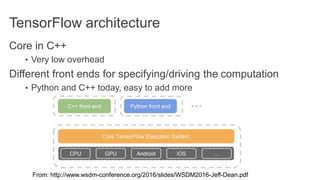
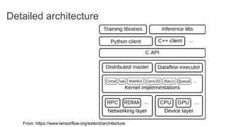
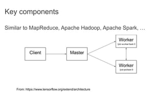
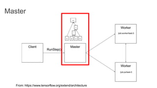
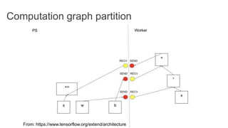
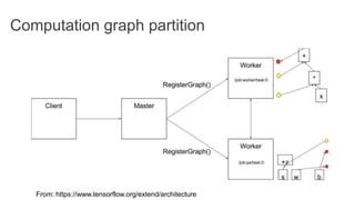
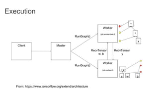
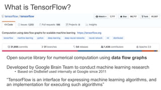
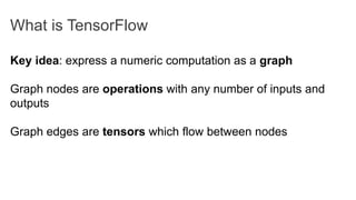
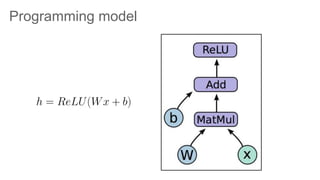
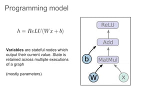
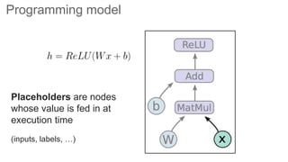
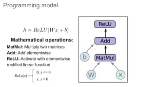
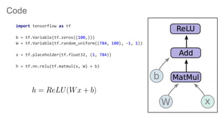
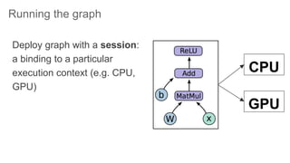
2. Today’s lecture
Abadi et al., “TensorFlow: A System for Large-Scale Machine
Learning”, OSDI 2016
(https://www.usenix.org/system/files/conference/osdi16/osdi16-abadi.pdf)
Crankshaw et al., “Clipper: A Low-Latency Online Prediction
Serving System”, NSDI 2017
(https://www.usenix.org/conference/nsdi17/technical-
sessions/presentation/crankshaw)
3. A short history of Neural Networks
1957: Perceptron (Frank Rosenblatt): one layer network neural
network
1959: first neural network to solve a real world problem, i.e.,
eliminates echoes on phone lines (Widrow & Hoff)
1988: Backpropagation (Rumelhart, Hinton, Williams): learning
a multi-layered network
4. A short history of NNs
1989: ALVINN: autonomous driving car
using NN (CMU)
1989: (LeCun) Successful application to recognize handwritten
ZIP codes on mail using a “deep” network
2010s: near-human capabilities for image recognition, speech
recognition, and language translation
5. Perceptron
Invented by Frank Rosenblatt (1957): simplified mathematical
model of how the neurons in our brains operate
From: http://www.andreykurenkov.com/writing/ai/a-brief-history-of-neural-nets-and-deep-learning/
6. Perceptron
Could implement AND, OR, but not XOR
From: http://www.andreykurenkov.com/writing/ai/a-brief-history-of-neural-nets-and-deep-learning/
7. Hidden layers
Hidden layers can find features within the data and allow
following layers to operate on those features
• Can implement XOR
From: http://www.andreykurenkov.com/writing/ai/a-brief-history-of-neural-nets-and-deep-learning/
9. Context (circa 2015)
Deep learning already claiming big successes
From: http://www.wsdm-conference.org/2016/slides/WSDM2016-Jeff-Dean.pdfz
Imagenet
challenge
classification
task
10. Context (circa 2015)
Deep learning already claiming big successes
Number of developers/researchers exploding
A “zoo” of tools and libraries, some of questionable quality…
11. What is TensorFlow?
Open source library for numerical computation using data flow graphs
Developed by Google Brain Team to conduct machine learning research
• Based on DisBelief used internally at Google since 2011
“TensorFlow is an interface for expressing machine learning algorithms, and
an implementation for executing such algorithms”
12. What is TensorFlow
Key idea: express a numeric computation as a graph
Graph nodes are operations with any number of inputs and
outputs
Graph edges are tensors which flow between nodes
14. Variables are stateful nodes which
output their current value. State is
retained across multiple executions
of a graph
(mostly parameters)
Programming model
17. Code
import tensorflow as tf
b = tf.Variable(tf.zeros((100,)))
W = tf.Variable(tf.random_uniform((784, 100), -1, 1))
x = tf.placeholder(tf.float32, (1, 784))
h = tf.nn.relu(tf.matmul(x, W) + b)
18. Running the graph
Deploy graph with a session:
a binding to a particular
execution context (e.g. CPU,
GPU)
CPU
GPU
19. End-to-end
So far:
• Built a graph using variables and placeholders
• Deploy the graph onto a session, i.e., execution environment
Next: train model
• Define loss function
• Compute gradients
20. Defining loss
Use placeholder for labels
Build loss node using labels and prediction
prediction = tf.nn.softmax(...) #Output of neural network
label = tf.placeholder(tf.float32, [100, 10])
cross_entropy = -tf.reduce_sum(label * tf.log(prediction), axis=1)
21. Gradient computation: Backpropagation
train_step = tf.train.GradientDescentOptimizer(0.5).minimize(cross_entropy)
tf.train.GradientDescentOptimizer is an Optimizer object
tf.train.GradientDescentOptimizer(lr).minimize(cross_entropy)
adds optimization operation to computation graph
TensorFlow graph nodes have attached gradient operations
Gradient with respect to parameters computed with
backpropagation … automatically
22. Design Principles
Dataflow graphs of primitive operators
Deferred execution (two phases)
1. Define program i.e., symbolic dataflow graph w/ placeholders
2. Executes optimized version of program on set of available devices
Common abstraction for heterogeneous accelerators
1. Issue a kernel for execution
2. Allocate memory for inputs and outputs
3. Transfer buffers to and from host memory
23. Dynamic Flow Control
Problem: support ML algos that contain conditional and
iterative control flow, e.g.
• Recurrent Neural Networks (RNNs)
• Long-Short Term Memory (LSTM)
Solution: Add conditional (if statement) and iterative (while
loop) programming constructs
24. TensorFlow high-level architecture
Core in C++
• Very low overhead
Different front ends for specifying/driving the computation
• Python and C++ today, easy to add more
From: http://www.wsdm-conference.org/2016/slides/WSDM2016-Jeff-Dean.pdf
25. TensorFlow architecture
Core in C++
• Very low overhead
Different front ends for specifying/driving the computation
• Python and C++ today, easy to add more
From: http://www.wsdm-conference.org/2016/slides/WSDM2016-Jeff-Dean.pdf
33. Fault Tolerance
Assumptions:
• Fine grain operations: “It is unlikely that tasks will fail so often that
individual operations need fault tolerance” ;-)
• “Many learning algorithms do not require strong consistency”
Solution: user-level checkpointing (provides 2 ops)
• save(): writes one or more tensors to a checkpoint file
• restore(): reads one or more tensors from a checkpoint file
35. Discussion
OpenMP/Cilk MPI MapReduce / Spark
Environment,
Assumptions
Single node, multiple
core, shared memory
Supercomputers
Sophisticate programmers
High performance
Hard to scale hardware
Commodity clusters
Java programmers
Programmer productivity
Easier, faster to scale up cluster
Computation
Model
Fine-grained task
parallelism
Message passing Data flow / BSP
Strengths Simplifies parallel
programming on multi-
cores
Can write very fast
asynchronous code
Fault tolerance
Weaknesses Still pretty complex,
need to be careful
about race conditions
Fault tolerance
Easy to end up with non-
deterministic code (if not
using barriers)
Not as high performance as MPI
Editor's Notes
3-D graph
Checklist
What we want to enable
What we have today
How we’ll get there
Neural network with one hidden layer
The function we are computing is on the left. Relu is an activation function that takes the max of 0 and your input, applies a nonlinearity to your network.
The graph on the right is how this function would look like in a tensorflow graph.
Let us break down the nodes in the graph into three types
We have two variables in this graph, the bias and W matrix.
What we mean by saying that variables are stateful is that they retain their current value over multiple executions, and it’s easy to restore saved values to variables.
Variables have a number of other useful features. They can be saved to disk during and after training, and gradient updates will by default apply over all the variables in your graph
Variables are still operations (nodes = operations!). When you run a variable you get the value of its state.
The variables in your graph are going to be your parameters
The second important node type is placeholders. If you have inputs into your network that depend on some external data, you want to be able to build your graph without depending on any real values yet, as those are passed in at run time.
Placeholders, unlike variables that have initial assignment, expect as arguments a data type and a shape of a tensor.
Inputs, labels
The other nodes are mathematical operations that you are familiar with. Matmul, addition, and relu are all operations in your graph that combine your inputs and parameters to produce new nodes.