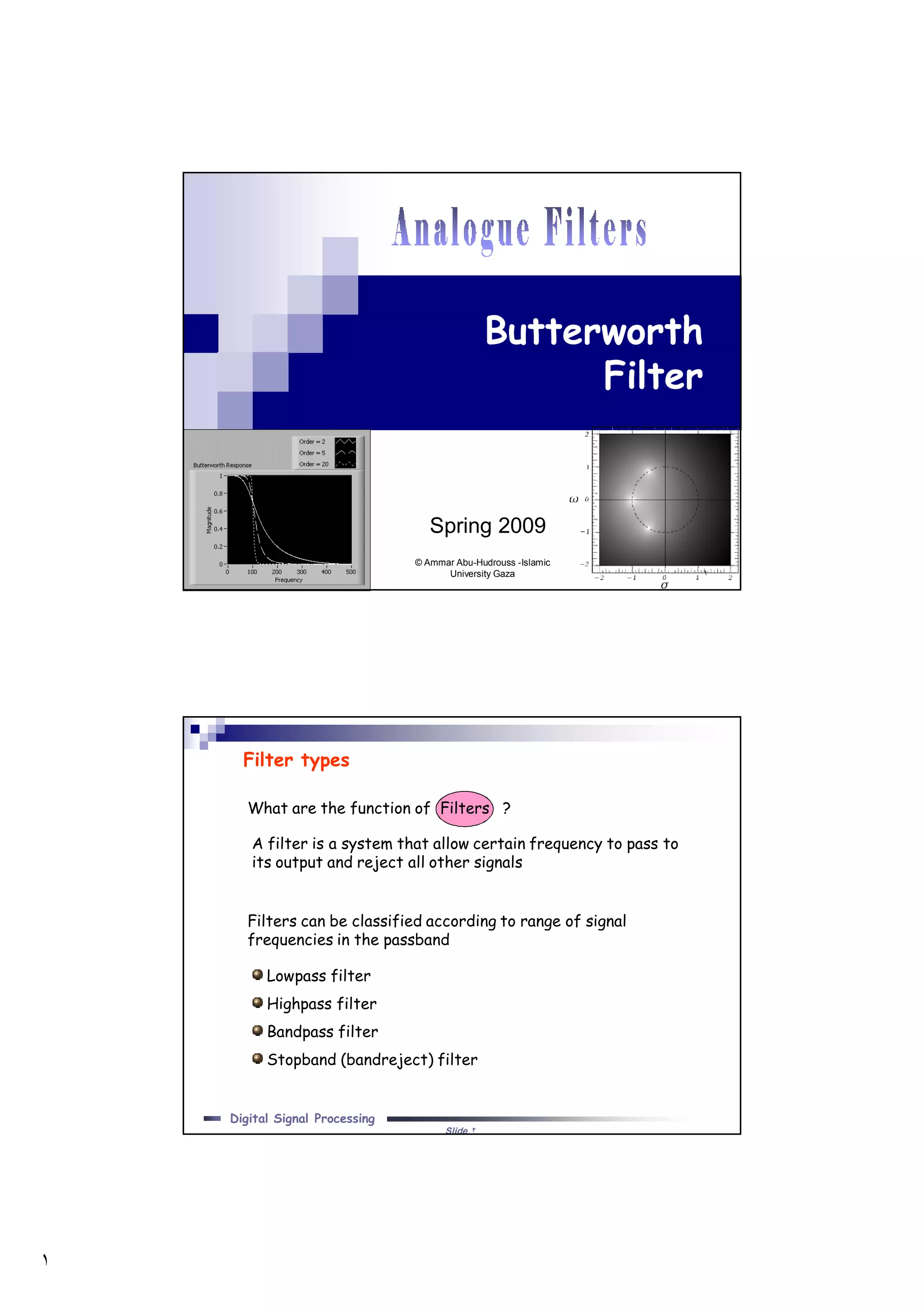
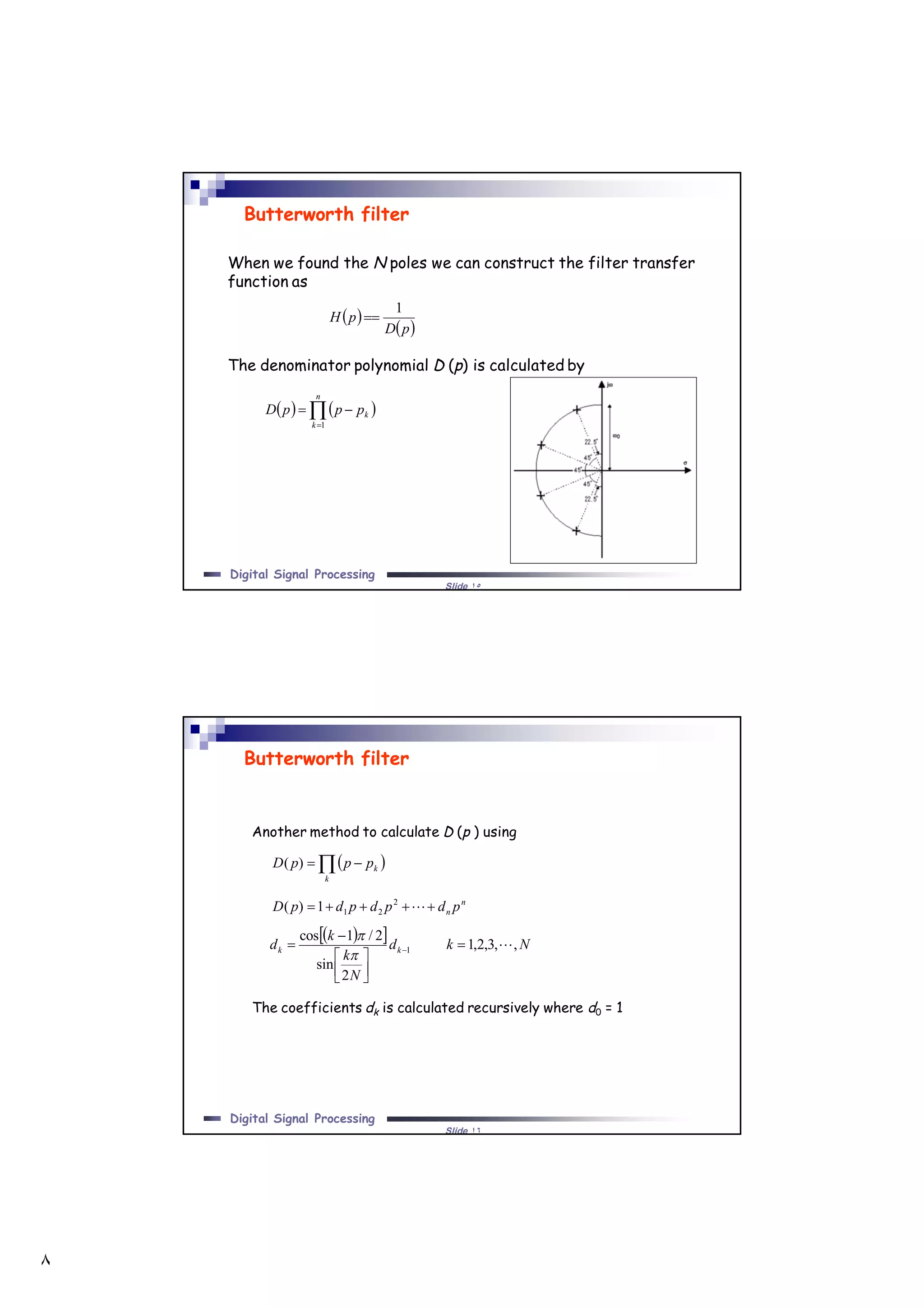
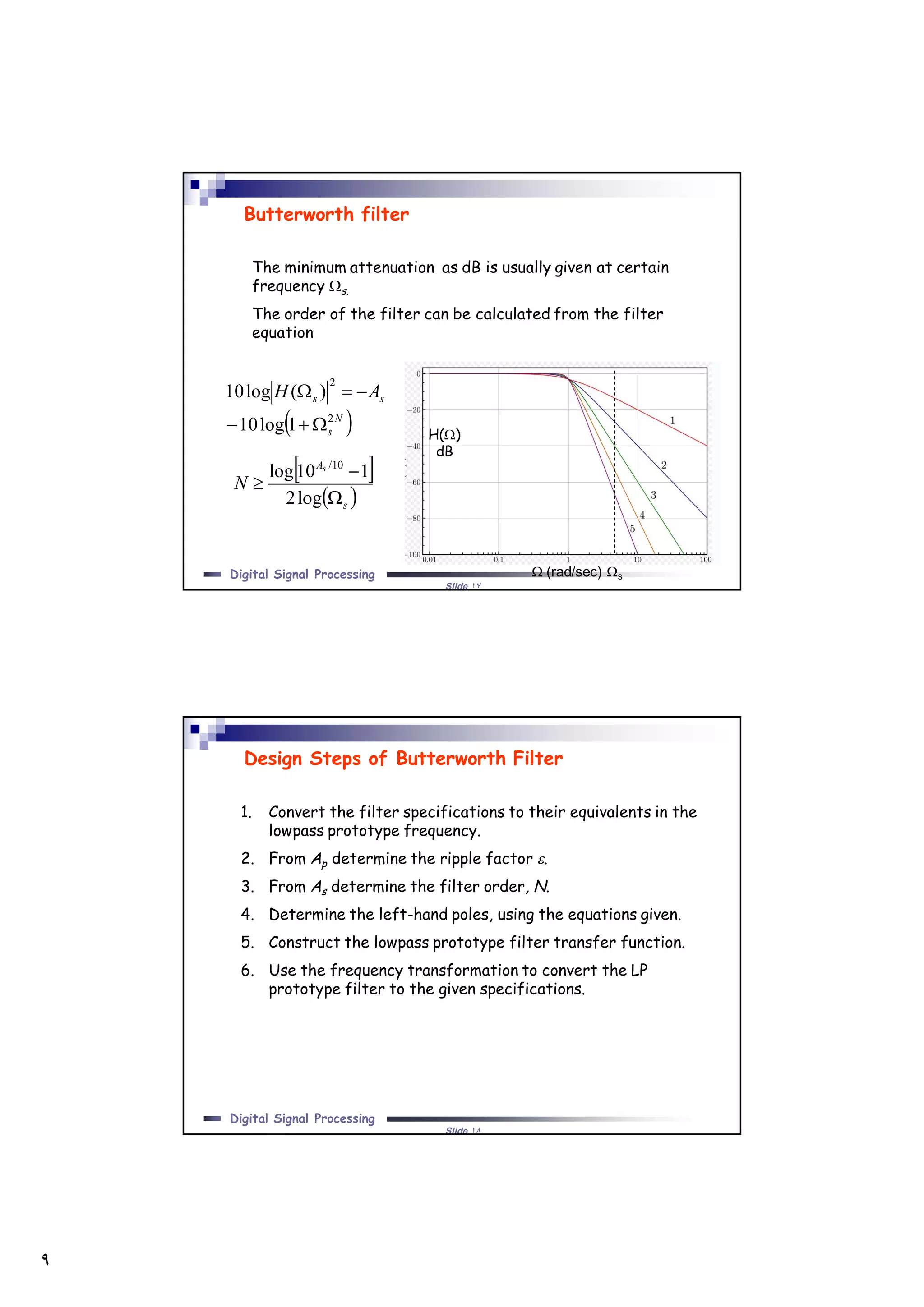
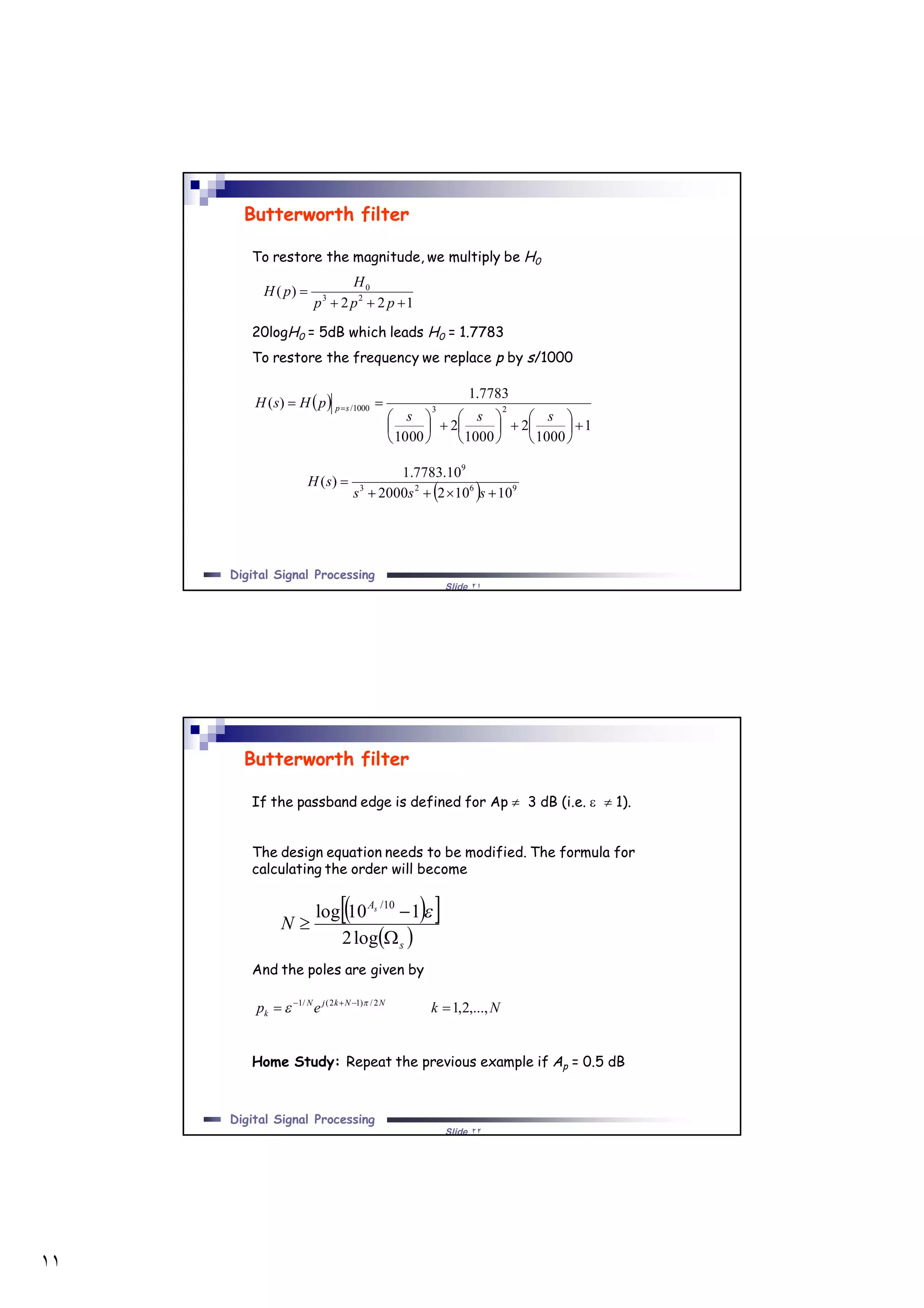
١
١
Butterworth
Filter
Spring 2009
© Ammar Abu-Hudrouss -Islamic
University Gaza
Slide ٢
Digital Signal Processing
What are the function of Filters ?
Filters can be classified according to range of signal
frequencies in the passband
Lowpass filter
Highpass filter
Bandpass filter
Stopband (bandreject) filter
A filter is a system that allow certain frequency to pass to
its output and reject all other signals
Filter types
٢
Slide ٣
Digital Signal Processing
Filter types
Slide ٤
Digital Signal Processing
Filter types according to its frequency response
Butterworth filter
Chebychev I filter
Chebychev II filter
Elliptic filter
Filter types
٣
Slide ٥
Digital Signal Processing
Butterworth filter
Ideal lowpass filter is shown in the figure
The passband is normalised to one.
Tolerance in passband and stopband are allowed to enable
the construction of the filter.
Slide ٦
Digital Signal Processing
Lowpass prototype filter
Lowpass prototype filter: it is a lowpass filter with
cutoff frequency p=1.
Lowpass
prototype
filter
Frequency
Transformation
Lowpass filter
Highpass filter
Bandpass filter
Bandreject filter
The frequency scale is normalized by p. We use  = / p.
٤
Slide ٧
Digital Signal Processing
Lowpass prototype filter
Notation
In analogue filter design we will use
s to denote complex frequency
to denote analogue frequency
p to denote complex frequency at lowpass prototype
frequencies.
 to denote analogue frequency at the lowpass prototype
frequencies.
Slide ٨
Digital Signal Processing
Magnitude Approximation of Analog Filters
 The transfer function of analogue filter is given as rational
function of the form
 The Fourier transform is given by
  nm
sdsdsdd
scscscc
sH n
n
m
mo






2
210
2
21
   
  n
n
n
m
m
m
o
js
djdjdd
cjcjcc
sHH


 


 


2
210
2
21
)(
   
 j
ejHH )(
٥
Slide ٩
Digital Signal Processing
Magnitude Approximation of Analog Filters
 Analogue filter is usually expressed in term of
 Example
 Consider the transfer function of analogue filter, find
      jHjHjH *2

 
22
1
2



ss
s
sH
       jsjs
ss
s
ss
s
sHsHjH 





22
1
22
1
22
2
 
42
1
2 4
2





jH
 
 
 


2


jH
jH
Slide ١٠
Digital Signal Processing
In order to approximate the ideal filter
1) The magnitude at  = 0 is normalized to one
2) The magnitude monotonically decreases from this value to
zero as ∞.
3) The maximum number of its derivatives evaluated at  = 0
are zeros.
This can be satisfied if
Butterworth filter
n
n
m
mo
DDD
CCCC
H 2
2
4
4
2
2
2
2
4
4
2
22
1
)(








Will have only even powers of , or
N
ND
H 2
2
2
1
1
)(




 2
jH
٦
Slide ١١
Digital Signal Processing
The following specification is usually given for a lowpass
Butterworth filter is
1) The magnitude of H0 at  = 0
2) The bandwidth p.
3) The magnitude at the bandwidth p.
4) The stopband frequency s.
5) The magnitude at the stopband frequency s.
6) The transfer function is given by
Butterworth filter
  N
ND
H
H 2
2
02
1
)(


Slide ١٢
Digital Signal Processing
To achieve the equivalent lowpass prototype filter
1) We scale the cutoff frequency to one using transformation
 = / p.
2) We scale the magnitude to 1 to one by dividing the magnitude
by H0 .
The transfer function become
We denotes D2N as  2 where  is the ripple factor, then
Butterworth filter
  N
ND
H 2'
2
2
1
1
)(


  N
H 22
2
1
1
)(



٧
Slide ١٣
Digital Signal Processing
If the magnitude at the bandwidth  = p = 1 is given as (1 - p)2
or −Ap decibels,
the value of 2 is computed by
If we choose Ap = -3dB   2 = 1. this is the most common case
and gives
Butterworth filter
pAH
p
2)(log20
2
1
 
pA
 2
1
1
log10

110
1.02
 pA

  N
H 2
2
1
1
)(


Slide ١٤
Digital Signal Processing
If we use the complex frequency representation
The poles of this function occurs at
Or in general
Poles occurs in complex conjugates
Poles which are located in the LHP are the poles of H(s)
Butterworth filter
 
 Njp
p
HpH
2/
22
1
1
)(

 
 






 
even,2,...,2,1
odd,2,...,2,1
2/12
2/2
nNke
nNke
p Nk
Nk
k 

Nkep NNkj
k 2,...,2,12/)12(
  
Nkep NNkj
k ,...,2,12/)12(
  
٨
Slide ١٥
Digital Signal Processing
When we found the N poles we can construct the filter transfer
function as
The denominator polynomial D (p) is calculated by
Butterworth filter
 
 pD
pH
1

   

n
k
kpppD
1
Slide ١٦
Digital Signal Processing
Butterworth filter
Another method to calculate D (p ) using
The coefficients dk is calculated recursively where d0 = 1
  
k
kpppD )(
n
n pdpdpdpD  2
211)(
   Nkd
N
k
k
d kk ,,3,2,1
2
sin
2/1cos
1 





 


٩
Slide ١٧
Digital Signal Processing
Butterworth filter
The minimum attenuation as dB is usually given at certain
frequency s.
The order of the filter can be calculated from the filter
equation
s (rad/sec)
H()
dB
 N
s
ss AH
2
2
1log10
)(log10


 
 s
As
N



log2
110log 10/
Slide ١٨
Digital Signal Processing
Design Steps of Butterworth Filter
1. Convert the filter specifications to their equivalents in the
lowpass prototype frequency.
2. From Ap determine the ripple factor .
3. From As determine the filter order, N.
4. Determine the left-hand poles, using the equations given.
5. Construct the lowpass prototype filter transfer function.
6. Use the frequency transformation to convert the LP
prototype filter to the given specifications.
١٠
Slide ١٩
Digital Signal Processing
Butterworth filter
Example:
Design a lowpass Butterworth filter with a maximum gain of 5 dB
and a cutoff frequency of 1000 rad/s at which the gain is at least
2 dB and a stopband frequency of 5000 rad/s at which the
magnitude is required to be less than −25dB.
Solution:
p = 1000 rad/s , s = 5000 rad/s,
By normalization,
p = p/ p = 1 rad/s,
s = s / p = 5 rad/s,
And the stopband attenuation As = 25+ 5 =30 dB
The filter order is calculated by
  3146.2
)5log(2
)110log( 10/



sA
N
Slide ٢٠
Digital Signal Processing
Butterworth filter
The pole positions are:
  
3,2,16/22
 
kep kj
k

   866.05.0,1,866.05.0,, 3/43/2
jjeeep jjj
k  
   866.05.01866.05.0)( jppjppD 
  11)( 2
 ppppD
122)( 23
 ppppD
Hence the transfer function of the normalized prototype
filter of third order is
122
1
)( 23


ppp
pH
١١
Slide ٢١
Digital Signal Processing
Butterworth filter
To restore the magnitude, we multiply be H0
20logH0 = 5dB which leads H0 = 1.7783
To restore the frequency we replace p by s/1000
122
)( 23
0


ppp
H
pH
 
1
1000
2
1000
2
1000
7783.1
)( 231000/


















 
sss
pHsH sp
  9623
9
101022000
10.7783.1
)(


sss
sH
Slide ٢٢
Digital Signal Processing
Butterworth filter
If the passband edge is defined for Ap  3 dB (i.e.   1).
The design equation needs to be modified. The formula for
calculating the order will become
And the poles are given by
Home Study: Repeat the previous example if Ap = 0.5 dB
  
 s
As
N



log2
110log 10/

Nkep NNkjN
k ,...,2,12/)12(/1
  


01analog filters

  • 1.
    ١ ١ Butterworth Filter Spring 2009 © AmmarAbu-Hudrouss -Islamic University Gaza Slide ٢ Digital Signal Processing What are the function of Filters ? Filters can be classified according to range of signal frequencies in the passband Lowpass filter Highpass filter Bandpass filter Stopband (bandreject) filter A filter is a system that allow certain frequency to pass to its output and reject all other signals Filter types
  • 2.
    ٢ Slide ٣ Digital SignalProcessing Filter types Slide ٤ Digital Signal Processing Filter types according to its frequency response Butterworth filter Chebychev I filter Chebychev II filter Elliptic filter Filter types
  • 3.
    ٣ Slide ٥ Digital SignalProcessing Butterworth filter Ideal lowpass filter is shown in the figure The passband is normalised to one. Tolerance in passband and stopband are allowed to enable the construction of the filter. Slide ٦ Digital Signal Processing Lowpass prototype filter Lowpass prototype filter: it is a lowpass filter with cutoff frequency p=1. Lowpass prototype filter Frequency Transformation Lowpass filter Highpass filter Bandpass filter Bandreject filter The frequency scale is normalized by p. We use  = / p.
  • 4.
    ٤ Slide ٧ Digital SignalProcessing Lowpass prototype filter Notation In analogue filter design we will use s to denote complex frequency to denote analogue frequency p to denote complex frequency at lowpass prototype frequencies.  to denote analogue frequency at the lowpass prototype frequencies. Slide ٨ Digital Signal Processing Magnitude Approximation of Analog Filters  The transfer function of analogue filter is given as rational function of the form  The Fourier transform is given by   nm sdsdsdd scscscc sH n n m mo       2 210 2 21       n n n m m m o js djdjdd cjcjcc sHH           2 210 2 21 )(      j ejHH )(
  • 5.
    ٥ Slide ٩ Digital SignalProcessing Magnitude Approximation of Analog Filters  Analogue filter is usually expressed in term of  Example  Consider the transfer function of analogue filter, find       jHjHjH *2    22 1 2    ss s sH        jsjs ss s ss s sHsHjH       22 1 22 1 22 2   42 1 2 4 2      jH         2   jH jH Slide ١٠ Digital Signal Processing In order to approximate the ideal filter 1) The magnitude at  = 0 is normalized to one 2) The magnitude monotonically decreases from this value to zero as ∞. 3) The maximum number of its derivatives evaluated at  = 0 are zeros. This can be satisfied if Butterworth filter n n m mo DDD CCCC H 2 2 4 4 2 2 2 2 4 4 2 22 1 )(         Will have only even powers of , or N ND H 2 2 2 1 1 )(      2 jH
  • 6.
    ٦ Slide ١١ Digital SignalProcessing The following specification is usually given for a lowpass Butterworth filter is 1) The magnitude of H0 at  = 0 2) The bandwidth p. 3) The magnitude at the bandwidth p. 4) The stopband frequency s. 5) The magnitude at the stopband frequency s. 6) The transfer function is given by Butterworth filter   N ND H H 2 2 02 1 )(   Slide ١٢ Digital Signal Processing To achieve the equivalent lowpass prototype filter 1) We scale the cutoff frequency to one using transformation  = / p. 2) We scale the magnitude to 1 to one by dividing the magnitude by H0 . The transfer function become We denotes D2N as  2 where  is the ripple factor, then Butterworth filter   N ND H 2' 2 2 1 1 )(     N H 22 2 1 1 )(   
  • 7.
    ٧ Slide ١٣ Digital SignalProcessing If the magnitude at the bandwidth  = p = 1 is given as (1 - p)2 or −Ap decibels, the value of 2 is computed by If we choose Ap = -3dB   2 = 1. this is the most common case and gives Butterworth filter pAH p 2)(log20 2 1   pA  2 1 1 log10  110 1.02  pA    N H 2 2 1 1 )(   Slide ١٤ Digital Signal Processing If we use the complex frequency representation The poles of this function occurs at Or in general Poles occurs in complex conjugates Poles which are located in the LHP are the poles of H(s) Butterworth filter    Njp p HpH 2/ 22 1 1 )(              even,2,...,2,1 odd,2,...,2,1 2/12 2/2 nNke nNke p Nk Nk k   Nkep NNkj k 2,...,2,12/)12(    Nkep NNkj k ,...,2,12/)12(   
  • 8.
    ٨ Slide ١٥ Digital SignalProcessing When we found the N poles we can construct the filter transfer function as The denominator polynomial D (p) is calculated by Butterworth filter    pD pH 1       n k kpppD 1 Slide ١٦ Digital Signal Processing Butterworth filter Another method to calculate D (p ) using The coefficients dk is calculated recursively where d0 = 1    k kpppD )( n n pdpdpdpD  2 211)(    Nkd N k k d kk ,,3,2,1 2 sin 2/1cos 1          
  • 9.
    ٩ Slide ١٧ Digital SignalProcessing Butterworth filter The minimum attenuation as dB is usually given at certain frequency s. The order of the filter can be calculated from the filter equation s (rad/sec) H() dB  N s ss AH 2 2 1log10 )(log10      s As N    log2 110log 10/ Slide ١٨ Digital Signal Processing Design Steps of Butterworth Filter 1. Convert the filter specifications to their equivalents in the lowpass prototype frequency. 2. From Ap determine the ripple factor . 3. From As determine the filter order, N. 4. Determine the left-hand poles, using the equations given. 5. Construct the lowpass prototype filter transfer function. 6. Use the frequency transformation to convert the LP prototype filter to the given specifications.
  • 10.
    ١٠ Slide ١٩ Digital SignalProcessing Butterworth filter Example: Design a lowpass Butterworth filter with a maximum gain of 5 dB and a cutoff frequency of 1000 rad/s at which the gain is at least 2 dB and a stopband frequency of 5000 rad/s at which the magnitude is required to be less than −25dB. Solution: p = 1000 rad/s , s = 5000 rad/s, By normalization, p = p/ p = 1 rad/s, s = s / p = 5 rad/s, And the stopband attenuation As = 25+ 5 =30 dB The filter order is calculated by   3146.2 )5log(2 )110log( 10/    sA N Slide ٢٠ Digital Signal Processing Butterworth filter The pole positions are:    3,2,16/22   kep kj k     866.05.0,1,866.05.0,, 3/43/2 jjeeep jjj k      866.05.01866.05.0)( jppjppD    11)( 2  ppppD 122)( 23  ppppD Hence the transfer function of the normalized prototype filter of third order is 122 1 )( 23   ppp pH
  • 11.
    ١١ Slide ٢١ Digital SignalProcessing Butterworth filter To restore the magnitude, we multiply be H0 20logH0 = 5dB which leads H0 = 1.7783 To restore the frequency we replace p by s/1000 122 )( 23 0   ppp H pH   1 1000 2 1000 2 1000 7783.1 )( 231000/                     sss pHsH sp   9623 9 101022000 10.7783.1 )(   sss sH Slide ٢٢ Digital Signal Processing Butterworth filter If the passband edge is defined for Ap  3 dB (i.e.   1). The design equation needs to be modified. The formula for calculating the order will become And the poles are given by Home Study: Repeat the previous example if Ap = 0.5 dB     s As N    log2 110log 10/  Nkep NNkjN k ,...,2,12/)12(/1    