The document describes a study that uses various machine learning techniques to build classifiers from imbalanced datasets. It applies 9 machine learning models (KNN, decision trees, random forest, SVM, etc.) to the original imbalanced dataset as well as two SMOTE-generated balanced datasets. It finds that models generally perform better on the balanced datasets, and that ensemble techniques combining top models from each dataset yield the best results, with an optimal model achieving an AUC of 0.7915. The study concludes that considering multiple perspectives through dataset balancing and ensemble methods leads to more robust classifiers.

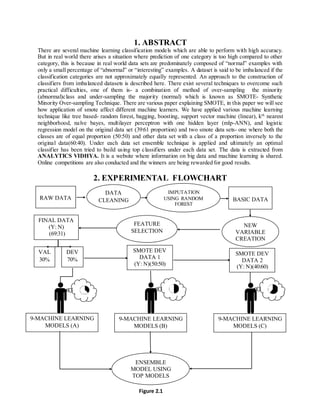
1. 1. ABSTRACT
There are several machine learning classification models which are able to perform with high accuracy.
But in real world there arises a situation where prediction of one category is too high compared to other
category, this is because in real world data sets are predominately composed of “normal” examples with
only a small percentage of “abnormal” or “interesting” examples. A dataset is said to be imbalanced if the
classification categories are not approximately equally represented. An approach to the construction of
classifiers from imbalanced datasets is described here. There exist several techniques to overcome such
practical difficulties, one of them is- a combination of method of over-sampling the minority
(abnormal)class and under-sampling the majority (normal) which is known as SMOTE- Synthetic
Minority Over-sampling Technique. There are various paper explaining SMOTE, in this paper we will see
how application of smote affect different machine learners. We have applied various machine learning
technique like tree based- random forest, bagging, boosting, support vector machine (linear), kth
nearest
neighborhood, naïve bayes, multilayer perceptron with one hidden layer (mlp-ANN), and logistic
regression model on the original data set (39:61 proportion) and two smote data sets- one where both the
classes are of equal proportion (50:50) and other data set with a class of a proportion inversely to the
original data(60:40). Under each data set ensemble technique is applied and ultimately an optimal
classifier has been tried to build using top classifiers under each data set. The data is extracted from
ANALYTICS VIDHYA. It is a website where information on big data and machine learning is shared.
Online competitions are also conducted and the winners are being rewarded for good results.
2. EXPERIMENTAL FLOWCHART
9-MACHINE LEARNING
MODELS (A)
VAL
30%
SMOTE DEV
DATA 1
(Y: N)(50:50)
SMOTE DEV
DATA 2
(Y: N)(40:60)
DEV
70%
RAW DATA BASIC DATA
DATA
CLEANING
IMPUTATION
USING RANDOM
FOREST
FINAL DATA
(Y: N)
(69:31)
FEATURE
SELECTION
NEW
VARIABLE
CREATION
9-MACHINE LEARNING
MODELS (B)
9-MACHINE LEARNING
MODELS (C)
ENSEMBLE
MODEL USING
TOP MODELS
Figure 2.1

2. 3. RESULT
3.1. RESULTS OF EACH MODELOVER THREE DATA SETS
3.1.1. RECURSIVE PARTITIONING
Table 3.1.1
Original Smote1 Smote2
Dev
AUC 0.8414 0.8956 0.9403
Val
AUC 0.6329 0.6776 0.6696
val pred Kappa
0 1
0 23 32 0.2724
1 21 109
val Pred Kappa
0 1
0 29 26 0.2464
1 35 95
val pred Kappa
0 1
0 31 24 0.2118
1 43 87
 As we deviate from original data set recursive partitioning model performs better in terms of AUC
 In validations it is not performing better and there is no significant difference between datasets in terms
AUC
 In fact the kappa values are decreasing as we deviate from original data set.
3.1.2. KTH NEAREST NEIGHBOR (KNN)
Table 3.1.2
Original Smote1 Smote2
Dev
AUC 0.9882 0.9973 0.9931

3. Val
AUC 0.6679 0.6681 0.6627
val pred Kappa
0 1
0 20 35 0.298
1 13 117
val pred Kappa
0 1
0 24 31 0.2165
1 29 101
val pred Kappa
0 1
0 26 29 0.1973
1 35 95
 KNN performs very well in all the development data sets therefore it over learn from the data.
 But in validation set invariably it performs poorly in terms of both AUC and kappa
 As we deviate from original data set, performance of KNN keeps on decreasing
3.1.3. MULTI LAYER PERCEPTRON WITH ONE HIDDEN LAYER (MLP)
Table 3.1.3
Original Smote1 Smote2
Dev
AUC 0.9986 0.9998 0.9998
Val
AUC 0.7106 0.5385 0.5929
val pred kappa
0 1
0 27 28 0.3518
1 20 110
val pred kappa
0 1
0 28 27 0.1567
1 44 86
val pred Kappa
0 1
0 36 19 0.2714
1 45 85
 MLP performs very well in all the development data sets,it also tries to over learn from the data
 In validation set MLP built on original data set performs well whereas in both the SMOTE based models
perform poorly.
 Another important aspect to be noted is that MLP learns poorly when proportions of classes are equal.

4. 3.1.4. SUPPORT VECTOR MACHINE
Table 3.1.4
Original Smote1 Smote2
Dev
AUC 0.9214 0.9638 0.9613
Val
AUC 0.7028 0.7038 0.698
val pred Kappa
0 1
0 19 36 0.3728
1 4 126
val pred kappa
0 1
0 32 23 0.26
1 39 91
val pred Kappa
0 1
0 26 29 0.2144
1 33 97
 SVM performs very well in all the development data sets.
 In validation it performs well to some extent, and smote1 gives better model among the three models.
 This shows that the target variable at equal proportions helps SVM model to perform better.
3.1.5. RANDOM FOREST
Table 3.1.5
Original Smote1 Smote2
Dev
AUC 1 1 1
Val

5. AUC 0.7101 0.7207 0.7175
val pred kappa
0 1
0 22 33 0.3565
1 11 119
val pred Kappa
0 1
0 32 23 0.3664
1 27 107
val pred Kappa
0 1
0 29 26 0.2995
1 29 101
 Invariably in all the data sets random forest tend to over fit.
 In validation set it performs well but there is no significant difference in three models in terms of AUC
and kappa.
3.1.6. BAGGING
Table 3.1.6
Original Smote1 Smote2
Dev
AUC 0.9578 0.9706 0.9769
Val
AUC 0.6833 0.7014 0.7055
val pred kappa
0 1
0 19 36 0.3328
1 6 124
val pred kappa
0 1
0 32 23 0.3478
1 29 101
val pred Kappa
0 1
0 25 30 0.3173
1 20 110
 As we deviate from the original data set i.e. if increase our samples bagging increases its performance.
 In validation set AUC keeps on increasing over the models.
 In terms of kappa values, performance by smote2 is lesser than other models.
3.1.7. BOOSTING
Table 3.1.7
Original Smote1 Smote2
Dev

6. AUC 1 1 1
Val
AUC 0.6814 0.6954 0.714
val pred kappa
0 1
0 23 33 0.3925
1 16 114
val pred kappa
0 1
0 30 25 0.2539
1 26 94
val pred Kappa
0 1
0 30 25 0.2976
1 31 99
 Invariably in all the data sets boosting tend to over fit.
 In validation set AUC values keeps on increasing as we deviate from original data set.
 In terms of kappa values model fitted on original data yields better result than the other model.
3.1.8. NAIVE BAYES
Table 3.1.8
Original Smote1 Smote2
Dev
AUC 0.7396 0.8106 0.7869
Val
AUC 0.6308 0.6171 0.6373
val pred kappa
0 1
0 22 33 0.2939
1 17 113
val pred kappa
0 1
0 21 34 0.2959
1 15 115
val pred Kappa
0 1
0 48 7 0.02743
1 108 22
 Naïve bayes performs best when the target variable is at equal proportion in development data set.
 In validation set AUC value is highest for smote-2 but the kappa value is too low. This is mainly because
naïve bayes tries to over learn the ‘0’ category therefore it predicts highest number of ‘0’ categories
among all the models.

7. 3.1.9. LOGISTIC REGRESSION
Table 3.1.9
Original Smote1 Smote2
Dev
AUC 0.8549 0.9171 0.9211
Val
AUC 0.6903 0.6849 0.6839
Val pred kappa
0 1
0 22 33 0.4238
1 5 125
val pred kappa
0 1
0 24 31 0.2959
1 22 108
val pred Kappa
0 1
0 24 31 0.2613
1 24 106
 Performance of Logistic regression keeps on increasing as we are deviating from original data set.
 In validation set model built on original data set is best among all the data set
3.2. CLUSTER ANALYSIS ON PROBABILITIES DERIVED FROM EACH
MODELFROM EACH DATA SET.
3.2.1. ORIGINAL DEVELOPMENT DATA SET
Figure 3.2.1

8. We have performed cluster analysis on validation set’s probabilities derived from different models
applied on original data set. We can observe that totally 4 cluster are formed.
Cluster1 Multilayer perceptron.
Cluster2 Recursive partitioning and naïve bayes
Cluster3 Kth nearest neighborhood and boosting
Cluster4 Logistic regression, svm, random forest and bagging
Using the prior information on the individual learner and the study from above cluster analysis we can
build better model by using ensemble technique on two best models from different cluster. For example
(1) By combining logistic regression and multilayer perceptron we get better kappa value of 0.4355
(2) By combining logistic regression and boosting we get better kappa value of 0.4284
3.2.2. SMOTE-1 DEVELOPMENT DATA (Y:N=50:50)
Figure 3.2.2
We can observe that totally 3 cluster are formed.
Cluster1 Multilayer perceptron.
Cluster2 Recursive partitioning, random forest,boosting and bagging
Cluster3 Kth nearest neighborhood,Logistic regression, svm and naïve bayes
 We can observe that when we ensemble boosting with bagging, which is from same cluster gives a kappa
value of 0.4376.
 When we ensemble boosting with MLP,which is from different cluster gives a kappa value of 0.4193

9. 3.2.3. SMOTE-2 DEVELOPMENT DATA (Y:N=40:60)
Figure 3.2.3
We can observe that totally 3 cluster are formed.
Cluster1 Naïve bayes
Cluster2 Multilayer perceptron
Cluster3
Kth
nearest neighborhood, logistic regression, recursive partitioning,
svm,random forest,boosting and bagging
In this case we can observe that when we ensemble logistic regression with bagging, which is from same
cluster is gives a kappa value of 0.4049
3.2.4. CLUSTER ANALYSIS ON ALL THE PREDICTIONPROBABILITY
Figure 3.2.4

10. Cluster1 naïve bayes model -2
Cluster2 mlp-1,2
Cluster3
Bagging models-1,2,3 , boosting models-1,2,3 , random forest models-1,2,3
and support vector machine models-1,2,3
Cluster4
logistic regression models-1,2,3, Kth nearest neighborhood models-1,2,3,
recursive partitioning model-1,2,3, mlp-3 and remaining naïve bayes-1,3
Here 1 represent original data set, 2 as smote-1 data set,3 as smote-2
4. FINAL MODEL
Table 4
KAPPA VALUES
MODELS original smote1 smote2
RECURSIVE PARTITIONING 0.2724 0.2464 0.2118
Kth NEAREST NEIGHBOURHOOD 0.298 0.2165 0.1973
MULTILAYER PERCEPTRON 0.3518 0.1567 0.2714
SUPPORT VECTOR MACHINE 0.3782 0.26 0.2144
RANDOM FOREST 0.3565 0.3664 0.2995
BAGGING 0.3328 0.3478 0.3173
BOOSTING 0.3925 0.2539 0.2976
NAÏVE BAYES 0.2939 0.2959 0.02743
LOGISTIC REGRESSION 0.4238 0.2959 0.2613
Using wrapper model treating each model’s probabilities as features for dependent variable we can extract
top most important models that clearly explains the dependent variable. The above table represents kappa
values of all the single models, the highlighted kappa values represents the important features (extracted
from the wrapper model) that explains the dependent variable.
Therefore the model built from the above highlighted variable gives a roc curve and a confusion matrix -

11. This optimum model gives an AUC value of 0.7915
Table 4.1
This gives a kappa value of 0.4706
5. CONCLUSION
 Among the 9 machine learning models KNN, MLP, random forest and boosting suffers from
over fitting.
 In terms of performance in validation set SVM, random forest, bagging, boosting is much better
than other models.
 In terms of uniqueness MLP and naïve bayes learns separately compared to other models,
specifically MLP is able to produce better result.
 Inherently logistic regression model on original data set is able to perform better.
 Similarly models like bagging are able to improve if we apply SMOTE.
 After applying ensemble technique over different models derived from the three data set , both
AUC and kappa value is optimum.
 This implies instead of learning from one perspective i.e. from original data set , if we are able to
create more data sets of different proportion using SMOTE and ensemble all the top models built
from each data set then we can build a classifier which can be applicable in long run and for a
wide variety of future data sets.
 Not only is this type ensemble technique applicable for imbalanced data set but also for a
balanced data set it can be applied to have more precise understanding and high prediction
power.
References
 Nitesh V. Chawla, Kevin W. Bowyer, Lawrence O. Hall , W. Philip Kegelmeyer , SMOTE: Synthetic
Minority Over-sampling Technique, Journal of Artificial Intelligence Research 16 (2002).
 Jiliang Tang, Salem Alelyani and Huan Liu, Feature Selection for Classification: A Review
 Trevor Hashtie, Robert Tibshirani, Jerome Friedman , Elements of statistical learning, Springer
Texts in Statistics
 Daniel J. Stekhoven, missForest, ETH Zurich seminar for statistics
 Paulo Cortez, Data Mining with Neural Networks and Support Vector Machines using the
R/rminer Tool, Department of Information Systems/R&D Centre, University of Minho, Portugal.
PREDICTED
TARGET
NO YES
NO 24 31
YES 5 125