Hippocampal ltp and contextual learning require surface diffusion of ampa receptors

0 0 M o n t h 2 0 1 7 | V O L 0 0 0 | N A T U R E | 1
Letter doi:10.1038/nature23658
Hippocampal LTP and contextual learning require
surface diffusion of AMPA receptors
A. C. Penn1,2,3
*, C. L. Zhang1,2
*, F. Georges1,2,4
, L. Royer1,2,†
, C. Breillat1,2
, E. Hosy1,2
, J. D. Petersen1,2,5
, Y. Humeau1,2
§ &
D. Choquet1,2,5
§
Long-term potentiation (LTP) of excitatory synaptic transmission
has long been considered a cellular correlate for learning and
memory1,2
. Early LTP (less than 1 h) had initially been explained
either by presynaptic increases in glutamate release3–5
or by direct
modification of postsynaptic AMPA (α-amino-3-hydroxy-5-
methyl-4-isoxazolepropionic acid) receptor function6,7
. Compelling
models have more recently proposed that synaptic potentiation
can occur by the recruitment of additional postsynaptic AMPA
receptors (AMPARs)8
, sourced either from an intracellular reserve
pool by exocytosis or from nearby extra-synaptic receptors pre-
existing on the neuronal surface9–12
. However, the exact mechanism
through which synapses can rapidly recruit new AMPARs during
early LTP remains unknown. In particular, direct evidence
for a pivotal role of AMPAR surface diffusion as a trafficking
mechanism in synaptic plasticity is still lacking. Here, using
AMPAR immobilization approaches, we show that interfering
with AMPAR surface diffusion markedly impairs synaptic
potentiation of Schaffer collaterals and commissural inputs to
the CA1 area of the mouse hippocampus in cultured slices, acute
slices and in vivo. Our data also identify distinct contributions
of various AMPAR trafficking routes to the temporal profile
of synaptic potentiation. In addition, AMPAR immobilization
in vivo in the dorsal hippocampus inhibited fear conditioning,
indicating that AMPAR diffusion is important for the early phase
of contextual learning. Therefore, our results provide a direct
demonstration that the recruitment of new receptors to synapses
by surface diffusion is a critical mechanism for the expression of
LTP and hippocampal learning. Since AMPAR surface diffusion
is dictated by weak Brownian forces that are readily perturbed by
protein–protein interactions, we anticipate that this fundamental
trafficking mechanism will be a key target for modulating synaptic
potentiation and learning.
Hebbian LTP is characterized by a prolonged increase in a synaptic
response that occurs upon robust, coincident activation of pre- and post-
synaptic neurons. The induction of canonical LTP proceeds by calcium
influxthroughpostsynapticN-methyl-D-aspartatereceptors(NMDARs)
and subsequent activation of calcium/calmodulin-dependent
kinase II (CaMKII)6,8
. However, despite decades of intense research on
synaptic plasticity focused on the Schaffer collateral and commissural
synapses, there is still ambiguity over how canonical LTP is ultimately
expressed13
. A substantial body of evidence suggests postsynaptic
mechanisms8
, where the prime candidates have been an increase in
the conductance or number of AMPARs6–8
. Synaptic recruitment of
additional receptors had initially been proposed to originate from
stimulus-induced AMPAR exocytosis from intracellular stores14–17
.
However, work from our laboratory and others has shown that there
is a large number of extra-synaptic surface AMPARs in hippocampal
neurons and that a substantial fraction of them diffuse almost freely
by Brownian motion before being reversibly confined and trapped at
synapses10,12
. Furthermore, activity-dependent activation of CaMKII
induces rapid immobilization of AMPARs at synapses10,18
, and recent
work implicates a pre-existing extra-synaptic receptor pool in the
expression of LTP19
. Both lateral movement and exocytosis of AMPARs
could indeed contribute to LTP20
. Together, this led us to directly
investigate the contribution of AMPAR surface diffusion to synaptic
potentiation.
We developed manipulations that crosslink surface AMPARs, thereby
preventing their diffusion on the cell membrane. First, we created
constructs to autonomously express recombinant biotin-tethered
AMPAR subunits 1 and 2 (ref. 21) (bAP::SEP::GluA1 and 2, where AP
indicates the biotin acceptor tag, bAP indicates the biotinylated AP tag
when co-expressed with the biotin ligase BirA, SEP is super-ecliptic
phluorin and GluA1 encodes subunit 1 of the AMPAR, also known as
Gria1), which we could surface crosslink by tetrameric biotin-binding
proteins (BBPs, approximately 60 kDa, Fig. 1a, b). We transfected
bAP::SEP::GluA subunits into cultured hippocampal neurons and
monitored their surface diffusion by fluorescence recovery after photo-
bleaching (FRAP). Brief pre-treatment of transfected cultures with
BBP NeutrAvidin significantly inhibited FRAP at dendritic spines
(Fig. 1c, d) only if both the acceptor peptide (AP) tag was included in
the construct and if the endoplasmic-reticulum-retained biotin ligase
(BirA-ER) was co-expressed (Fig. 1d). Therefore, we could effectively
manipulate postsynaptic AMPAR surface diffusion by a specific
crosslinking approach. Similar NeutrAvidin-induced immobilization of
AMPARs was obtained when measured by tracking bAP–SEP–GluA2
diffusion with quantum dots (Extended Data Fig. 1).
Much of our current understanding of LTP mechanisms comes from
experiments on in vitro hippocampal slice preparations. We achieved
effective molecular replacement of endogenous receptors by delivering
bAP::SEP::GluA2 into CA1 neurons of slice cultures from GluA2-
knockout mice (Gria2−/−
). In wild-type mice (Gria2+/+
), principal
neurons of the hippocampus predominantly express hetero-tetrameric
AMPARs composed of the GluA1 and GluA2 subunits, which have a
linear current–voltage (I–V) relationship (Fig. 1e, grey). By contrast,
AMPAR currents in the absence of GluA2 (Gria2−/−
) are inwardly
rectifying (Fig. 1e, red)22
. Expression of bAP::SEP::GluA2 faithfully
restored linear I–V relationships in the Gria2−/−
slices for both synaptic
currents (Fig. 1e, top, green) and extra-synaptic glutamate uncaging
currents to near wild-type levels (Fig. 1e, bottom, green). We also con-
firmed that BBPs could effectively diffuse through organotypic slices
and bind specifically to molecularly replaced neurons (Extended Data
Fig. 2a). Importantly, following this expression manipulation, we could
1
University of Bordeaux, Interdisciplinary Institute for Neuroscience, UMR5297, F-33000 Bordeaux, France. 2
CNRS, Interdisciplinary Institute for Neuroscience, UMR 5297, F-33000 Bordeaux,
France. 3
Sussex Neuroscience, School of Life Sciences, University of Sussex, Brighton BN1 9QG, UK. 4
University of Bordeaux, Institute of Neurodegenerative Diseases, CNRS UMR 5293, 146 Rue
Léo Saignat, 33076 Bordeaux, France. 5
Bordeaux Imaging Center, UMS 3420 CNRS, US4 INSERM, University of Bordeaux, Bordeaux, France. †Present address: Department of Biology, Brandeis
University, 415 South Street, Waltham, Massachusetts, USA.
*These authors contributed equally to this work.
§These authors jointly supervised this work.
© 2017 Macmillan Publishers Limited, part of Springer Nature. All rights reserved.

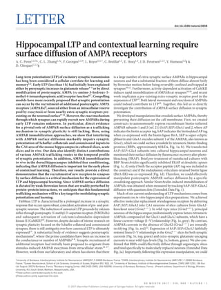
2 | N A T U R E | V O L 0 0 0 | 0 0 m o n t h 2 0 1 7
LetterRESEARCH
obtain stable excitatory postsynaptic potentials (EPSPs, Extended Data
Fig. 2b) and reliably induce synaptic potentiation by applying high-
frequency stimulation (HFS) (Fig. 2a).
We next evaluated the effect of AMPAR crosslinking on synaptic
transmission and potentiation. Acute pre-treatment with NeutrAvidin
followed by wash of transfected slice cultures to crosslink only pre-
existing surface AMPARs had no detectable effects on basal synaptic
transmission (Fig. 1f, top and middle; Extended Data Fig. 2c, e) or
surface AMPAR levels (Fig. 1f, bottom). However, this pre-treatment
with NeutrAvidin completely abolished the short-term potentiation
(STP) induced by HFS (Fig. 2b). Since we could not detect significant
effects of NeutrAvidin on postsynaptic depolarization during HFS
(Extended Data Fig. 2d) or on the average size of the EPSP during
the baseline (Extended Data Fig. 2e), this impaired potentiation
was probably not a result of failure to reach the induction threshold.
Furthermore, the amplitude and time course of synaptic NMDA
receptor currents in bAP::SEP::GluA2-replacement cells were unaffected
by the crosslink manipulation (Fig. 1f, top; Extended Data Fig. 2f).
Finally, we confirmed that the effect of NeutrAvidin required specific
interactions with bAP–SEP–GluA2 by showing that potentiation
was normal in neurons co-expressing myc–SEP–GluA2 (which does
not bind NeutrAvidin) and BirA-ER in NeutrAvidin-treated slices
(Extended Data Fig. 3a). These results suggest that diffusion of a pre-
existing surface pool of postsynaptic AMPARs has a critical role in the
expression of synaptic potentiation.
While fully abolishing STP, crosslink pre-treatment still allowed
the slow development of a significant, albeit smaller, early LTP (eLTP;
Fig. 2b). This prompted us to evaluate the contribution of different
AMPAR trafficking steps to shaping the temporal profile of synaptic
potentiation. Previous reports described intact STP following
intracellular injection of neurotoxins, which prevent postsynaptic
membrane fusion events and LTP14
, or more recently following the
specific knockout of the exocytic machinery17
. After reproducing this
ourselves using tetanus toxin light chain (TeTx, Fig. 2c; Extended Data
Fig. 3b), we hypothesized that the exocytosis of new AMPARs to the
cell surface contributes to the expression of synaptic potentiation only
at later time periods. Consistent with this, gradual run-up of synaptic
transmission after HFS in slices pre-incubated with NeutrAvidin was
blocked by either intracellular TeTx (Fig. 2d) or N-ethylmaleimide
(Extended Data Fig. 3c). Newly exocytosed receptors might also require
surface diffusion as an intermediate step for synaptic recruitment since
exocytosis has been proposed to occur away from synapses15,16,20
.
Indeed, the presence of low concentrations of NeutrAvidin in the extra-
cellular recording solution following NeutrAvidin pre-treatment of
slices prevented both STP and eLTP (Fig. 2e). Since we could not detect
an effect of our postsynaptic manipulation on presynaptic parameters
(Extended Data Fig. 4), these data reveal a preferential contribution of
mobile postsynaptic AMPARs sourced from pre-existing surface and
intracellular pools to establishing STP and sustaining eLTP, respectively
(Extended Data Fig. 5).
To confirm that AMPAR diffusion is an important trafficking step for
endogenous AMPARs during the expression of synaptic potentiation,
we used an antibody crosslinking approach. In cultured hippocampal
neurons, single-layer crosslink using an immunoglobulin G (IgG)
against GluA2 effectively limited the surface diffusion of AMPARs
(Extended Data Fig. 1 and 6) without modifying their endocytosis or
phosphorylation status (Extended Data Fig. 7). Neither pre-injection
of crosslinking anti-GluA2 IgG nor the monovalent control fragment
antigen binding (Fab) into CA1 of acute hippocampal slices had any
effect on basal synaptic transmission (Extended Data Fig. 8a, c–f). By
contrast, strong attenuation of HFS-induced STP was observed with
the anti-GluA2 IgG, but not the Fab, without affecting the HFS-induced
decrease in the paired-pulse ratio at an interstimulus interval of 200 ms,
which measures the pre-synaptic component of synaptic potentiation
(Extended Data Fig. 8b). Notably, eLTP induced by HFS or theta-burst
stimulation (TBS) was completely abolished when the anti-GluA2 IgG
was infused continuously in the slice (Fig. 3b, c; Extended Data Fig. 9).
We then confirmed that endogenous AMPAR diffusion is an impor-
tant trafficking step for eLTP in vivo (Fig. 3d). In contrast to the Fab
Figure 1 | Biotin-tethered AMPARs are effectively crosslinked by
NeutrAvidin to prevent their surface diffusion. a, Construct for dual
expression of AP–SEP–GluA and BirA-ER. IRES, internal ribosome entry
site. b, Strategy to crosslink bAP–SEP–GluA. c, Example images (top)
and graph showing mean FRAP curves, fits and standard error bands
(bottom) for control (Ctrl) and pre-treatment with NeutrAvidin (50 nM
for 2 min). For the example images, low pixel intensity values are white and
high pixel intensity values are black. d, Receptor mobile fraction in spines
of cells expressing bAP::SEP::GluA1 and bAP::SEP::GluA2 is reduced by
NeutrAvidin pre-treatment and depends on the AP tag and BirA-ER.
e, Molecular replacement with bAP–SEP–GluA2 in CA1 neurons. Example
AMPAR current traces from Schaffer collateral (SC) synapse stimulation
(top) or by one-photon glutamate uncaging on the soma (bottom).
MNI-Glu, 4-methoxy-7-nitroindolinyl (MNI)-caged glutamate. f, Pre-
treating slices with NeutrAvidin (100 nM for 45 min) caused no detectable
effect on: AMPA/NMDA ratios (top); evoked excitatory postsynaptic
conductances (middle); or glutamate (glut.) uncaging responses (bottom).
Bar graphs show marginal means with 83% confidence intervals (d) or
mean with s.e.m. error bars and data points (e, f). expts., experiments.
Statistical significance was assessed by mixed model nested ANOVA (d),
one-way ANOVA (e) or two-way ANOVA with Holm–Bonferroni post hoc
tests (f). NS, not significant; **P < 0.01; ***P < 0.001.

0 0 M o n t h 2 0 1 7 | V O L 0 0 0 | N A T U R E | 3
Letter RESEARCH
fragments (Fig. 3e) and control IgG (Fig. 3g), injection of anti-GluA2
IgG into the CA1 area of the dorsal hippocampus (Fig. 3f) caused a
marked attenuation of field EPSP potentiation following HFS at the
commissural CA1 input (Fig. 3h).
The dorsal hippocampus is a key structure for acquiring and memo-
rizing contextual aspects of fear memories23,24
and these processes have
been tied to AMPAR trafficking and synaptic potentiation in vivo25–27
.
Therefore, we reasoned that crosslinking surface AMPARs in the adult
dorsal hippocampus could impair the ability of mice to form contextual
fear memories.
Compared to anti-GluA2 Fab fragments and denatured IgG (Fig. 4a),
mice injected with anti-GluA2 IgG into the dorsal hippocampus exhib-
ited half the level of freezing when re-exposed to a fear-conditioned
context a day later (context A in Fig. 4a). After 2–3 days of recovery,
a second contextual conditioning task with the same mice resulted
in robust fear learning (context C in Fig. 4a). None of the mouse
groups exhibited contextual generalization (context B in Fig. 4a).
The effect of IgG was not a temporary impairment of the mice to
express conditioned fear responses, since all groups performed well
in hippocampus-independent, cued fear memory tests (Fig. 4b). We
ruled out a more general impairment of hippocampus function by the
anti-GluA2 IgG by infusing the antibodies before testing and showing
that recall of contextual fear memories was similar between anti-GluA2
IgG and Fab (Fig. 4c).
Our experiments demonstrate that recruitment of diffusing surface
AMPARs is an essential mechanism for eLTP, both in brain slices and
Figure 2 | Crosslink reveals surface diffusion as a critical step in the
synaptic delivery of AMPARs during synaptic potentiation. Top,
scheme illustrates experimental protocols on organotypic hippocampal
slices. a–e, Left, example whole-cell voltage traces and summary plots
of mean normalized EPSP slope ± s.e.m. Middle, cumulative histograms
for average normalized EPSP slope during STP (2) and LTP (3). Right,
models of experimental manipulations. a, Robust STP and LTP following
HFS under control conditions (four experiments). b, Detectable
HFS-induced LTP but not STP in slices pre-treated with 100 nM
NeutrAvidin (five experiments). c, Severe attenuation of LTP but not STP
with 0.5 μM intracellular TeTx. d, e, No detectable change in EPSP slope
after HFS when 100 nM NeutrAvidin pre-treatment is combined with
either: TeTx in intracellular recording solution (d); or continuous infusion
of 10 pM NeutrAvidin in the external recording solution (e) (three
experiments). aCSF, artificial cerebrospinal fluid. Statistical significance
was assessed by repeated-measures ANOVA with Holm–Bonferroni post
hoc tests (a–e). NS, not significant; *P < 0.05; **P < 0.01.

4 | N A T U R E | V O L 0 0 0 | 0 0 m o n t h 2 0 1 7
LetterRESEARCH
in vivo, and that it underlies early phases of hippocampal-dependent
fear learning. Our observations provide direct evidence for a model
in which rapid but temporary recruitment of AMPARs from a sur-
face pool to synaptic sites by lateral movement and activity-dependent
trapping at the postsynaptic density mediates the earlier phase of
synaptic potentiation. This would then be followed by replenishment
of the extracellular pool by exocytosis of AMPARs, which also need to
diffuse to reach synaptic sites and sustain synaptic potentiation. That
manipulating AMPAR surface diffusion in vivo specifically affects
learning without modifying basal transmission offers a new approach
to influencing synaptic memory.
Online Content Methods, along with any additional Extended Data display items and
Source Data, are available in the online version of the paper; references unique to
these sections appear only in the online paper.
received 31 January 2016; accepted 21 July 2017.
Published online 13 September 2017.
1. Takeuchi, T., Duszkiewicz, A. J. & Morris, R. G. The synaptic plasticity and
memory hypothesis: encoding, storage and persistence. Phil. Trans. R. Soc.
Lond. B 369, 20130288 (2013).
2. Nicoll, R. A. A brief history of long-term potentiation. Neuron 93, 281–290 (2017).
3. MacDougall, M. J. & Fine, A. The expression of long-term potentiation:
reconciling the preists and the postivists. Phil. Trans. R. Soc. Lond. B 369,
20130135 (2013).
4. Padamsey, Z. & Emptage, N. Two sides to long-term potentiation: a view
towards reconciliation. Phil. Trans. R. Soc. Lond. B 369, 20130154 (2013).
5. Yang, Y. & Calakos, N. Presynaptic long-term plasticity. Front. Synaptic Neurosci.
5, 8 (2013).
6. Lisman, J., Yasuda, R. & Raghavachari, S. Mechanisms of CaMKII action in
long-term potentiation. Nat. Rev. Neurosci. 13, 169–182 (2012).
7. Lu, W. & Roche, K. W. Posttranslational regulation of AMPA receptor trafficking
and function. Curr. Opin. Neurobiol. 22, 470–479 (2012).
8. Granger, A. J. & Nicoll, R. A. Expression mechanisms underlying long-term
potentiation: a postsynaptic view, 10 years on. Phil. Trans. R. Soc. Lond. B 369,
20130136 (2013).
9. Huganir, R. L. & Nicoll, R. A. AMPARs and synaptic plasticity: the last 25 years.
Neuron 80, 704–717 (2013).
10. Opazo, P. et al. CaMKII triggers the diffusional trapping of surface AMPARs
through phosphorylation of stargazin. Neuron 67, 239–252 (2010).
11. Chater, T. E. & Goda, Y. The role of AMPA receptors in postsynaptic
mechanisms of synaptic plasticity. Front. Cell. Neurosci. 8, 401 (2014).
12. Opazo, P. & Choquet, D. A three-step model for the synaptic recruitment of
AMPA receptors. Mol. Cell. Neurosci. 46, 1–8 (2011).
13. Bliss, T. V. & Collingridge, G. L. Expression of NMDA receptor-dependent LTP in
the hippocampus: bridging the divide. Mol. Brain 6, 5 (2013).
14. Lledo, P. M., Zhang, X., Südhof, T. C., Malenka, R. C. & Nicoll, R. A. Postsynaptic
membrane fusion and long-term potentiation. Science 279, 399–403 (1998).
15. Park, M., Penick, E. C., Edwards, J. G., Kauer, J. A. & Ehlers, M. D. Recycling
endosomes supply AMPA receptors for LTP. Science 305, 1972–1975
(2004).
16. Patterson, M. A., Szatmari, E. M. & Yasuda, R. AMPA receptors are exocytosed in
stimulated spines and adjacent dendrites in a Ras-ERK-dependent manner
during long-term potentiation. Proc. Natl Acad. Sci. USA 107, 15951–15956
(2010).
Figure 3 | Antibody crosslink of endogenous GluA2 attenuates LTP
of CA1 field EPSPs in vitro and in vivo. a, Acute slice experimental
setup and antibody labelling controls. Ab, antibody. Stim., stimulator.
b, c, Protocol (top), example traces (middle) and summary plots of mean
normalized field EPSP slope ± s.e.m. No stable synaptic potentiation
following HFS (b) or TBS (c) is observed when anti-GluA2 IgG pre-
injection is combined with continuous infusion of the antibody.
Cumulative histograms for STP and LTP are presented in Extended
Data Fig. 9. d, In vivo experimental protocol and histological controls.
VHC, ventral hippocampal commissure. e–h, LTP recordings following
injection of: anti-GluA2 Fab (e); anti-GluA2 IgG (f); or control IgG (g).
Left, mean normalized field EPSP slope ± s.e.m. Right, example voltage
traces before and after HFS. h, Bar graph of the means with s.e.m. error
bars and data points for the normalized field EPSP slope potentiation
calculated from the data in Fig. 3e–g. Statistical significance was assessed
by one-way ANOVA with Holm–Bonferroni post hoc tests (h). NS, not
significant; *P < 0.05; **P < 0.01.

0 0 M o n t h 2 0 1 7 | V O L 0 0 0 | N A T U R E | 5
Letter RESEARCH
17. Wu, D. et al. Postsynaptic synaptotagmins mediate AMPA receptor exocytosis
during LTP. Nature 544, 316–321 (2017).
18. Borgdorff, A. J. & Choquet, D. Regulation of AMPA receptor lateral movements.
Nature 417, 649–653 (2002).
19. Granger, A. J., Shi, Y., Lu, W., Cerpas, M. & Nicoll, R. A. LTP requires a reserve
pool of glutamate receptors independent of subunit type. Nature 493,
495–500 (2013).
20. Makino, H. & Malinow, R. AMPA receptor incorporation into synapses during
LTP: the role of lateral movement and exocytosis. Neuron 64, 381–390 (2009).
21. Howarth, M., Takao, K., Hayashi, Y. & Ting, A. Y. Targeting quantum dots to
surface proteins in living cells with biotin ligase. Proc. Natl Acad. Sci. USA 102,
7583–7588 (2005).
22. Williams, K. Modulation and block of ion channels: a new biology of
polyamines. Cell. Signal. 9, 1–13 (1997).
23. Liu, X. et al. Optogenetic stimulation of a hippocampal engram activates fear
memory recall. Nature 484, 381–385 (2012).
24. McHugh, T. J. et al. Dentate gyrus NMDA receptors mediate rapid pattern
separation in the hippocampal network. Science 317, 94–99 (2007).
25. Takemoto, K. et al. Optical inactivation of synaptic AMPA receptors erases fear
memory. Nat. Biotechnol. 35, 38–47 (2017).
26. Kessels, H. W. & Malinow, R. Synaptic AMPA receptor plasticity and behavior.
Neuron 61, 340–350 (2009).
27. Whitlock, J. R., Heynen, A. J., Shuler, M. G. & Bear, M. F. Learning induces
long-term potentiation in the hippocampus. Science 313, 1093–1097 (2006).
Figure 4 | Impairment of a hippocampal-
dependent learning task by infusion of
crosslinking anti-GluA2 IgG. Shaded data are
controls for baseline freezing levels. Unshaded
data were used for hypothesis testing.
a, b, Selective effects on contextual (a) versus
cued (b) fear learning. a, Left, antibody infusion
sites. Right, pre-conditioning infusion of anti-
GluA2 IgG reduces freezing to conditioned
context A (square). Context A (square),
B (hexagon) and C (circle) indicate the different
contexts. b, Cued fear learning was robust
for all antibodies. c, No detectable difference
in freezing to conditioned context between
antibodies for pre-test infusions. All bar graphs
show means ± s.e.m. error bars. Data points are
shown where data are compared using statistics.
Statistical significance was assessed by two-
way repeated-measures ANOVA with Holm–
Bonferroni post hoc tests. NS, not significant;
**P < 0.01; ***P < 0.001. The mouse brain
drawing is reproduced with permission from
The Mouse Brain Atlas, K. B. J. Franklin and
G. Paxinos, page 74, Copyright Elsevier (2007).
Supplementary Information is available in the online version of the paper.
Acknowledgements We would like to thank A. Ting (MIT) for providing the
BirA-ER cDNA; E. Normand for histology; H. el Oussini for helping with acute
slice experiments; A. Lacquemant, A. Gautier, M. Deshors and others at the
Pôle In vivo in the IINS for animal husbandry; the Plateforme Génotypage in
Neurocentre Magendie; M. Carta for insightful discussions; R. Sprengel for
providing the Gria2-knockout mice; E. Gouaux for providing the anti-GluA2
antibodies, A. Carbone for data she obtained on a short-term EMBO fellowship.
The help of the Bordeaux Imaging Center, part of the national infrastructure
France BioImaging, granted by ANR-10INBS-04-0, is acknowledged. This work
was funded by: EMBO long-term fellowship ALTF 129-2009 (A.C.P.); European
Commission Marie Curie Actions FP7-PEOPLE-2010-IEF-273567 (A.C.P.),
Medical Research Council Career Development Award fellowship
MR/M020746/1 (A.C.P.), funding from the Ministère de l’Enseignement
Supérieur et de la Recherche, Centre National de la Recherche Scientifique, the
Conseil Régional d'Aquitaine, the Agence Nationale pour la Recherche Grant
Nanodom and the ERC grants nano-dyn-syn and ADOS to D.C.
Author Contributions A.C.P. performed molecular biology, imaging, slice
culture and transfection, designed and executed slice electrophysiology
experiments (all pertaining to the avidin–biotin crosslinking experiments) and
wrote the paper. Y.H. and C.L.Z. performed acute slice electrophysiology using
the antibody-mediated crosslinking approach. C.L.Z. performed surgeries and
behavioural experiments. F.G. performed in vivo electrophysiology experiments.
C.B. performed molecular and cell biology. J.D.P. performed antibody feeding
experiments. E.H. performed single-particle tracking and Q-dot experiments.
L.R. performed some imaging experiments. A.C.P. and Y.H. analysed the data.
D.C. and Y.H. conceived and supervised the study. All authors discussed the
results and contributed to the manuscript.
Author Information Reprints and permissions information is available
at www.nature.com/reprints. The authors declare no competing financial
interests. Readers are welcome to comment on the online version of the
paper. Publisher’s note: Springer Nature remains neutral with regard
to jurisdictional claims in published maps and institutional affiliations.
Correspondence and requests for materials should be addressed to
D.C. (daniel.choquet@u-bordeaux.fr).
Reviewer Information Nature thanks R. C. Malenka and the other anonymous
reviewer(s) for their contribution to the peer review of this work.

LetterRESEARCH
Methods
Reagents. Monoclonal whole IgG1-κand Fab fragments recognizing the extra-
cellular domain of GluA2 (clones 15F1 and 14B11, gifts from E. Gouaux), were
prepared using the purified GluA2 receptor in detergent solution as the antigen28
.
Control antibody for in vivo LTP experiments was polyclonal goat anti-rat IgG
(112-005-071, Jackson). Antibodies were stored at −80 °C and at 2.9–5.8 mg ml−1
in phosphate-buffered saline (PBS) containing (in mM): NaCl (50), sodium
phosphate (30, pH 7.4). For the denatured antibody control, the anti-GluA2 IgG
was incubated at 100 °C for 10 min. The anti-GFP whole IgG1-κwas from murine
clones 7.1 and 13.1 (11814450001, Roche). The antibody lyophilizate was reconsti-
tuted at 2.9 mg ml−1
in water and the buffer was exchanged by dialysis (overnight at
4 °C, 3500 MWCO) with PBS and the concentration re-adjusted to approximately
2.9 mg ml−1
.
The unlabelled, non-glycosylated form of avidin (NeutrAvidin) was purchased
from Invitrogen. Recombinant light chain of tetanus toxin was either purchased
from Quadratech Diagnostics or obtained as a gift from T. Galli. All solutions were
prepared in MilliQ water (18.2 M·cm) with salts purchased from Sigma-Aldrich.
Chemicals used for intracellular patch-clamp recording solutions were trace metal
grade purity. All drugs were purchased from Tocris Bioscience.
Molecular biology. An Ig κ-chain signal sequence (METDTLLLWVLLLW
VPGSTGDG), AP tag (GGLNDIFEAQKIEWHEGATG) and SEP were cloned
in-frame with the 5′-end of the coding sequence for the mature rat GluA1 and 2
subunit proteins. The entire open reading frames (ORFs) were cloned upstream
(5′) of an encephalomyocarditis virus (EMCV) internal ribosome entry site (IRES)
sequence. The BirA-ER coding sequence21
(a gift from A. Ting) was then cloned
to the 3′end of the IRES such that the start codon of the BirA-ER signal sequence
corresponded to the 11th ATG of the IRES sequence. Doxycycline-dependent
expression of the resulting dual-construct bAP::SEP::GluA was achieved by cloning
the entire AP::SEP::GluA IRES BirA-ER sequence into the multiple cloning site of
the pBI vector (BD Bioscience) and co-transfecting it with approximately equal
molar quantities of rtTA-transactivator. The GluA2 subunit used was edited
at the Q/R site (R607), unedited at the R/G site (R764) and the ligand-binding
domain splice variant was flop except for residue S775 (flip), where amino acid
numbering corresponds to the coding sequence of the immature GluA2 peptide
(NP_001077280.1). The GluA1 subunit used was a flip splice variant. Plasmid
DNA was prepared using endotoxin-free MaxiPreps (Qiagen). All constructs were
verified by restriction enzyme digest patterns and Sanger DNA sequencing.
Animals. GluA2-knockout mice29
used for slice culture experiments were bred
on a Swiss-type NMRI background, where the impact of the mutation on weight,
height, growth and fertility were weaker than on the original background strain.
Gria2−/−
pups identified by genotyping were obtained from heterozygote matings.
In vivo recordings and behaviour experiments were performed on 2–3-month-old
male C57BL6/J mice, housed in 12/12 light/dark with ad libitum feeding. Every
effort was made to minimize the number of animals used and their suffering. The
experimental designs and all procedures were in accordance with the European
guide for the care and use of laboratory animals and the animal care guidelines
issued by the animal experimental committee of Bordeaux Universities (CE50;
A5012009).
Dissociated neuron cultures. Banker cultures of hippocampal neurons from E18
Sprague–Dawley rat embryos of either sex were prepared at a density of 200,000
cells per 60-mm dish on poly-l-lysine pre-coated 1.5H coverslips (Marienfeld,
cat. no. 117580). Neuron cultures were maintained in Neurobasal medium
supplemented with 2 mM l-glutamine and 1×Neuromix supplement (PAA). After
48 h, 5 μM Ara-C (Sigma-Aldrich) was added to the culture medium. Astrocyte
feeder layers were prepared from the embryos the same age at a density of 20,000
to 40,000 cells per 60-mm dish (per the horse serum batch used) and cultured in
MEM (Fisher Scientific, cat. no. 21090-022) containing 4.5 g l−1
glucose, 2 mM
l-glutamine and 10% horse serum (Invitrogen) for 14 days.
Fluorescence recovery after photobleaching. Banker cultures were transfected
at 11 days in vitro (DIV) using Effectene (Qiagen). Doxycycline (1 μg ml−1
) was
added to the culture medium 24–48 h before experiments using inducible GluA2
constructs. Coverslips of transfected neurons (14–16 DIV) were mounted in a Ludin
chamber (Life Imaging Services) and transferred to an inverted microscope (Leica,
DMI 6000B) maintained at near-physiological temperature with a microscope
temperature control system (Life Imaging Services, Cube 2). The chamber was
perfused at 1 mg ml−1
(Gilson MiniPuls3) with extracellular solution containing
(in mM): NaCl (145), KCl (3.5), MgCl2 (2), CaCl2 (2), d-glucose (10), HEPES
(10) (pH 7.4, approximately 300 mOsm) and the preparation was observed
through a 63×oil objective (Leica, HCX PL APO CS, Iris NeutrAvidin 1.4-0.6).
Transfected cells were identified under epifluorescence (Leica EL6000) and illumi-
nated with 473 nm laser light using a high-speed spinning disk confocal scanner
unit (Yokogawa CSU22) for acquisition. Emission was captured with an electron
multiplying charge-coupled device (EMCCD) camera (Photometrics Quantem
512SC) and data were stored on the hard disk of a personal computer (DELL
Precision, Precision PWS690). Hardware was controlled with MetaMorph software
(Molecular Devices, v.7.1.7) and ILAS system software (Roper).
Images of SEP–GluA1-expressing neurons were acquired before and after
perfusion of 2 ml of fluorescently labelled biotin-binding proteins and then washed
for 5 min with Tyrode’s solution. Following the wash, using an exposure time of
0.5 s, the protocol consisted of: (1) acquiring 11 images at 0.67-s intervals; (2)
photobleaching the regions of interest (ROI); then (3) acquiring 40 images at 0.67-s
intervals and a further 55 images at 5-s intervals. For bleaching, we used a 5 ms
pulse of 488 nm laser light (Coherent Sapphire CDRH 100 mW) set to approxi-
mately 3.7 mW laser power at the back of the objective, which was sufficient to
reduce fluorescence by approximately 50%. A FRAP head (Roper/Errol) was used
to scan ROIs (about 0.690 μm diameter) with the bleaching laser. ROIs were posi-
tioned over a small number of independent spines across the field of view. Finally,
at the end of the experiment, we obtained an image before and after application of
membrane impermeant GFP quencher (5 mM Trypan red) to confirm that most of
the SEP fluorescence was on the cell surface. Time-lapse images were corrected for
XY-drift observational and bleach-pulse photobleaching30
using macros in either
MetaMorph (Molecular Devices) or ImageJ (http://imagej.nih.gov/ij/). ROIs of
fixed diameter (10 pixels, equivalent to 2.3 μm) were then carefully positioned over
each bleached spine head and the integrated or mean fluorescence intensity was
measured for every image. The fluorescence intensity for each ROI was subjected
to full-scale normalization by subtracting the average fluorescence intensity of
the pre-bleach images and dividing the result by the fluorescence of the first post-
bleach image.
Organotypic slice preparation and transfection. Hippocampi were dissected
from Gria2−/−
mice (either sex) at postnatal age 6–8 days in modified Gey’s
balancedsaltsolutionasdescribedpreviously31
.Transversesliceswerecutwithatissue
chopper (McIlwain) and positioned on small membrane segments (FHLC01300,
Millipore) and culture inserts (PICM0RG50, Millipore) in 6-well plates containing
1 ml per well slice culture medium, which was minimum essential medium
(MEM) supplemented with 15% heat-inactivated horse serum, 0.25 mM ascorbic
acid, 3 mM l-glutamine, 1 mM CaCl2, 1 mM MgSO4, 25 mM HEPES and 5 g l−1
d-glucose. Slices were maintained in an incubator at 34 °C with 5% CO2 and the
culture medium was replaced every 3–4 days. One week after plating, slices were
individually transferred to the chamber of an upright microscope (Eclipse FN1,
Nikon) where cells were co-transfected with Tet-on bAP::SEP::GluA2 and trans-
activator plasmids by single-cell electroporation (SCE)32
. In some experiments,
soluble tdTomato was also co-transfected to aid visualization of transfected cells.
Before commencing SCE, the microscope chamber was washed with 70% ethanol
and allowed to dry. A face mask was always used during the following procedures
and hands were regularly washed with 70% ethanol. During SCE, the chamber
contained sterile-filtered bicarbonate-containing Tyrode’s solution maintained at
ambient temperature and atmospheric conditions without perfusion. Bicarbonate-
containing Tyrode’s solution was composed of (in mM): NaCl (145), KCl (3.5),
CaCl2 (2.5), MgCl2 (1.3), HEPES (10), d-glucose (10), NaHCO3 (2) and sodium
pyruvate (1) (pH 7.3, 300 mOsm). Patch pipettes (approximately 8 MOhm) pulled
from glass capillaries (GB150F-8P, Science Products GmbH) were filled with
potassium-based solution (in mM): K-methanesulfonate (135), NaCl (4), HEPES
(10), EGTA (0.06), CaCl2 (0.01), MgCl2 (2), Na2-ATP (2) and Na-GTP (0.3) (pH
7.3, 280 mOsm) supplemented with plasmid DNA (total 10–33 ng μl−1
). After
obtaining loose-patch seals, electroporation was achieved by delivering 12 V at
100–200 Hz for 0.25–0.5 s (pulse-width 0.25–0.5 ms) using a constant voltage
stimulus isolator (IsoFlex, A.M.P.I.). On returning slices to the incubator, culture
media was supplemented with 10 μg ml−1
gentamicin, 1 μg ml−1
doxycycline and
10 μM d-biotin until experiments were preformed 2–3 weeks later. We attempted
to electroporate 5–10 CA1 neurons per slice with a typical success rate of 50%.
Organotypic slice electrophysiology. On the day of the experiment, organotypic
slices were transferred to a storage chamber containing carbogen (95% O2 / 5%
CO2)-bubbled artificial cerebral spinal fluid (aCSF) (in mM): NaCl (125), NaHCO3
(25), NaH2PO4 (1.25), KCl (2.5), CaCl2 (2), MgCl2 (2), d-glucose (10) and sodium
pyruvate (1). A dialysis device (3,500 molecular weight cut-off, Slide-A-Lyzer
MINI, Thermo Scientific) containing 0.25 ml of avidin Texas red conjugate was
included in the storage chamber to quench free-biotin from the slices for at least
45 min. For the crosslink, slices were then individually transferred to a culture
insert in a 35 mm culture dish containing 1 ml bicarbonate-containing Tyrode’s
solution with 100 nM NeutrAvidin and incubated at ambient temperature and
atmospheric conditions for 45 min followed by washing in bicarbonate-containing
Tyrode’s solution before electrophysiology experiments. For the control, incubation
was without NeutrAvidin (where the vehicle was Tyrode’s solution). Prior to any
electrophysiological recordings of electrically evoked synaptic responses, CA3 was
cut off to prevent seizures. The order of recordings was randomized for (blinded)
NeutrAvidin versus vehicle pre-treatment experiments.

Letter RESEARCH
For patch-clamp experiments, transfected Gria2−/−
slices were then transferred
to the microscope chamber perfused with carbogen (95% O2 / 5% CO2)-bubbled
recording aCSF maintained at approximately 30 °C by an in-line solution heater
(WPI). For recordings of LTP (Fig. 2), the aCSF contained (in mM): NaCl (125),
NaHCO3 (25), KCl (2.5), CaCl2 (4), MgSO4 (4), d-glucose (10), sodium pyruvate
(1), picrotoxin (0.005), 2-chloroadenosine (0.005), CGP-52432 (0.002) and ascor-
bic acid (0.25). A tungsten parallel bipolar stimulation electrode (about 100 μm
separation) was positioned in CA1 stratum radiatum close to the border with CA2.
Electrode placement and patching was visually guided by observing the prepara-
tion with oblique illumination of infrared light through a 40×water immersion
objective (NIR Apo 40×/0.80W, Nikon) and 1–2×optical zoom. Patch pipettes
(approximately 5 MOhm) for whole-cell current-clamp recordings were filled with
potassium-based intracellular solution (recipe as described above for SCE) but with
the addition of 0.15 mM spermine. After achieving a gigaohm seal, cells were main-
tained in cell-attached configuration for 5 min before breaking in. After opening
the cell, stimulation (40 μs) intensity (around 10 V) and polarity were adjusted to
obtain a small EPSP, mean peak amplitude 1.9 ± 0.13 mV (mean ± s.d.). Analogue
voltage signals were filtered online at 10 kHz, digitized at 50 kHz and stored directly
to the computer hard disk either using an EPC-10 USB controlled by Patchmaster
software (HEKA Electronik) from a computer workstation running Windows XP
(Microsoft), or using a MultiClamp 700B (Axon Instruments) controlled by ACQ4
v0.9.3 (http://www.acq4.org/) from a computer workstation running Windows 7
(Microsoft). Strictly 2 min after going whole-cell, the LTP recording was started
and consisted of: (1) stimulation at 0.1 Hz for 2 min to establish the baseline;
(2) 100 Hz for 1 s repeated 3 times at 20-s intervals (HFS); and (3) stimulation
at 0.1 Hz for 40 min to record post-HFS EPSP potentiation. For pseudo-HFS
recordings, the stimulator was switched off during the induction protocol in step
2. Short baseline recordings were necessary to prevent washout of LTP in slice
culture whole-cell recordings. LTP protocols were limited to once per slice. The
ensemble average obtained for every 3 traces was differentiated and filtered at
0.333 kHz (4-pole Bessel filter). The peak signal within 2–10 ms from the start
of the stimulus artefact in the resulting traces corresponded to the steepest slope
measurement, which is proportional to the underlying peak current (dV/dt ∝ I).
These values were routinely normalized to the measured pre-artefact membrane
potential to obtain more accurate slope measurements proportional to the under-
lying conductance. Peaks in the filtered first derivative had a latency of 4.6 ± 1.2 ms
(mean ± s.d.) from the onset of the stimulation artefact and were on average, an
amplitude equating to 18.0 ± 8.0 (mean ± s.d.) standard deviations of the pre-
stimulus baseline noise.
For whole-cell voltage clamp recordings of synaptic AMPAR rectification,
AMPA:NMDA ratios and evoked EPSC amplitudes, the recording aCSF instead
contained (in mM): NaCl (125), NaHCO3 (25), KCl (3.5), CaCl2 (5), MgCl2 (1),
d-glucose (10) and sodium pyruvate (1), picrotoxin (0.05), gabazine (0.002). Patch
pipettes (approximately 3–5 MOhm) for whole-cell voltage clamp recordings were
filled with a caesium-based intracellular solution containing (in mM): caesium
methanesulfonate (135), NaCl (4), HEPES (10), QX-314 Cl (3), BAPTA (1), EGTA
(0.6), CaCl2 (0.1), MgCl2 (2), Na2-ATP (2), Na-GTP (0.3) and spermine (0.15)
(pH 7.3, 290 mOsm). Voltage-clamp recordings were filtered online at 5 kHz and
digitized at 25 kHz. For AMPA:NMDA ratios, around 30 evoked EPSCs were
acquired and averaged at holding potentials of −70 and +40 mV. The ratio was
calculated from the peak current at −70 mV over the current measured at +40 mV
with a delay of 50 ms after the start of the stimulus artefact. In recordings of synaptic
AMPAR rectification only, aCSF was further supplemented with 0.1 mM D-APV to
inhibit NMDAR-mediated currents and around 30 evoked EPSCs were acquired
and averaged at holding potentials of −60, +30 and 0 mV. After subtraction of
0 mV traces, rectification index was calculated as the ratio of peak conductance
measurements at +30 mV over −60 mV. For basal transmission, peak synaptic
conductance measurements were obtained from evoked EPSCs recorded at holding
potentials between −70 and −60 mV using stimulation intensities of approximately
10 V. In all voltage clamp recordings, a calculated and experimentally verified liquid
junction potential of approximately +9 mV was corrected online.
For single-photon glutamate uncaging, voltage clamp recordings were
performed at room temperature without bath perfusion, in Tyrode’s solution
(recipe as described above for SCE) supplemented with (in mM): MNI-glutamate
(0.5), D-APV (0.1), picrotoxin (0.05), cyclothiazide (0.02) and TTX (0.001),
(pH 7.3, 300 mOsm). A caesium-based intracellular solution as described above
was used for voltage-clamp recordings but without BAPTA and with 0.001 mM
MK-801(+). Single-photon glutamate uncaging was achieved by pulses (5 ms)
of a 405 nm laser (0.4 mW) focused through a 60×water immersion objective
(NIR Apo 60×/1.00W, Nikon). The laser spot position was positioned with
galvanometric mirrors by a FRAP head (Roper) controlled using ILAS system
software in Metamorph (Molecular Devices). Rectification was measured and
calculated as described above for synaptic recordings.
Whole-cell recordings of NMDAR-mediated currents were evoked by electrical
stimulation of the Schaffer Collaterals. Recordings were performed at 30–32 °C and
a holding potential of −60 mV. The recording aCSF contained (in mM): NaCl (125),
NaHCO3 (25), KCl (2.5), CaCl2 (4), MgCl2 (4), d-glucose (10) and sodium pyruvate
(1), picrotoxin (0.05), NBQX (0.01), gabazine (0.002) and CGP-52432 (0.002).
Patch pipettes (approximately 3–5 MOhm) were filled with a caesium-based intra-
cellular solution containing (in mM): caesium methanesulfonate (135), NaCl (4),
HEPES (10), QX-314 Cl (3), EGTA (0.6), CaCl2 (0.1), MgCl2 (2), Na2-ATP (2)
and Na-GTP (0.3) (pH 7.3, 290 mOsm). Decay of the EPSC currents was fit by
a two-component exponential decay with offset initially using the Chebyshev
algorithm, where the fit parameters were then used as starting values for further
optimization by the Levenberg–Marquardt algorithm.
Throughout the paper, for clear presentation the stimulus artefact was blanked
out. Slice electrophysiology data was analysed in Stimfit v.0.13 (https://github.
com/neurodroid/stimfit/wiki/Stimfit) using custom Python modules (see Code
availability).
Confocal imaging in slice culture. Organotypic slices were prepared, transfected,
dialysed and pre-treated with biotin-binding protein as for the experiments illus-
trated in Fig. 2, except that we used 500 nM AlexFluor(AF)-633 conjugate of
Streptavidin (Molecular Probes) instead of unlabelled NeutrAvidin. After 45 min
incubation with Streptavidin AF-633, slices were washed in Tyrodes solution
(3 ×15 min) and fixed with 4% paraformaldehyde/0.2% glutaraldehyde in PBS.
Slices were then washed in PBS and water before mounting between a glass slide
and coverslip with Fluoromount-G mounting medium (Southern Biotech).
Samples were imaged through a 63×oil objective with the same spinning disk
confocal microscope described for the FRAP experiments. Streptavidin AF-633,
tdTomato and bAP::SEP::GluA2 were excited sequentially at each 0.2 μm z-step
using 635, 532 and 473 nm lasers respectively. Emitted light was captured with
100 ms exposure times and each z-step image represents an average of 50 frames.
Acute slice electrophysiology. For field recordings, we prepared hippocampus-
containing acute slices from C57BL6/J mice (8–9 weeks old). Briefly, mice
were anaesthetized with a mixture of ketamine/xylazine (100 and 10 mg kg−1
,
respectively), and cardiac-perfused with ice-cold, oxygenated sucrose-based
solution containing (in mM): 220 Sucrose, 2 KCl, 26 NaHCO3, 1.15 NaH2PO4,
10 glucose, 0.2 CaCl2, 6 MgCl2. The brains were rapidly removed, and cut in the
same sucrose-based solution using a vibratome (VT1200S, Leica Microsystems,
USA). Sagittal slices (350 μm) were transferred to an incubation chamber for
45 min at 34 °C, which contained a recording aCSF solution (mM): 124 NaCl, 3
KCl, 26 NaHCO3, 1.25 NaH2PO4, 10 glucose, 2 CaCl2, 1 MgCl2. After incubation,
the slices were maintained at room temperature in oxygenated aCSF for at least
30 min.
Hippocampal slices were recorded in a perfusion chamber continuously
perfused with warm (33.5 °C), carbogen (95% O2 / 5% CO2)-bubbled recording
aCSF using a peristaltic pump (Ismatec). A bipolar twisted platinum/iridium wire
electrode (50 μm diameter, FHC) was positioned in stratum radiatum of CA1
region, allowing the afferent Schaffer collateral–commissural pathway from the
CA3 to CA1 region to be stimulated. The field EPSPs (fEPSPs) were recorded from
stratum radiatum of CA1 area, using glass electrodes (approximately 2–3 MOhm)
pulled from borosilicate glass tubing (Harvard Apparatus; 1.5 mm OD × 1.17 mm
ID) and filled with aCSF. Pulses were delivered at 10-s intervals by Clampex 10.4
(Molecular Devices), and current was set using a stimulus isolator (Isoflex, AMPI)
to obtain 30–40% of the maximum fEPSP. To induce LTP we used either a HFS
(1 s at 100 Hz) repeated 3 times with an interval of 20 s, or TBS consisting of
10 bursts (4 pulses at 100 Hz) repeated at 5 Hz delivered 4 times with 10-s intervals.
Data were recorded with a Multiclamp700B (Axon Instruments) and acquired with
Clampex 10.4. The slope of the field excitatory postsynaptic potential (fEPSP) was
measured using clampfit with all values normalized to a 10-min baseline period.
All experiments done with field recording were with no pharmacology.
For whole-cell recordings, mice were cardiac-perfused with ice-cold, carbogen
(95% O2/5% CO2)-bubbled NMDG-based cutting solution containing (in mM):
93 NMDG, 93 HCl, 2.5 KCl, 1.2 NaH2PO4, 30 NaHCO3, 25 glucose, 10 MgSO4,
0.5 CaCl2, 5 sodium ascorbate, 3 sodium pyruvate, 2 thiourea and 12 mM N-acetyl-
l-cysteine (pH 7.3–7.4, with osmolarity of 300–310 mOsm). The sagittal slices
(350 μm) were prepared in the ice-cold and oxygenated NMDG cutting solution
described above, then transferred to an incubation chamber containing the same
NMDG cutting solution for 15 min at 34 °C. Before recording, the slices were main-
tained at room temperature for at least 45 min in carbogen (95% O2/5% CO2)-
bubbled aCSF containing (mM): 92 NaCl, 2.5 KCl, 1.2 NaH2PO4, 30 NaHCO3,
20 HEPES, 25 glucose, 2 MgSO4, 2 CaCl2, 5 sodium ascorbate, 3 sodium pyruvate,
2 thiourea and 12 mM N-acetyl-l-cysteine (pH 7.3–7.4, with osmolarity of
300–310 mOsm).
After CA3 regions were removed, the hippocampal slices were recorded in a
perfusion chamber and continuously perfused with warm (33.5 °C), carbogen

LetterRESEARCH
(95% O2/5% CO2)-bubbled recording aCSF (mM): 124 NaCl, 2.7 KCl, 2 CaCl2,
1.3 MgSO4, 26 NaHCO3, 1.25 NaH2PO4, 18.6 glucose, and 2.25 ascorbic acid.
Neurons in the CA1 region were visually identified with infrared video micros-
copy using an upright microscope equipped with a 60×objective. Patch electrodes
(4–5 M) were pulled from borosilicate glass tubing and filled with a low-chloride
solution containing (in mM): 140 caesium methylsulfonate, 5 QX314-Cl, 10
HEPES, 10 phosphocreatine, 4 Mg-ATP and 0.3 Na-GTP (pH adjusted to 7.25 with
CsOH, 295 mOsm). To evoke the EPSC, the stimulating electrode was positioned in
stratum radiatum of CA1 region. All whole-cell recording experiments were
performed in the presence of gabazine (10 μM) to block the GABA-A receptors.
To acquire the AMPA and NMDA EPSCs ratios, the ratio was calculated from
the peak current at −70 mV over the current measured at +50 mV with a delay
of 200 ms after the start of the stimulus artefact. For recording the NMDA EPSCs
only, CNQX (50 μM) was also included in the recording ACSF.
For antibody application, before field recording or whole-cell recording, an
injecting pipette (approximately 2–3 MOhm) was filled with either anti-GluA2
Fab (0.29 mg ml−1
dialysed against aCSF), anti-GluA2 IgG (0.29 mg ml−1
dialysed
against aCSF) or aCSF vehicle, and infused into the stratum radiatum at CA1 region
by using a constant air pressure (55–65 mbar) maintained in a tubing (around
1–1.2 m length, 0.8 mm ID) connected with a 1 ml syringe. After 30 min of injec-
tion, we removed the injection pipette, and started field recording in the injected
area and the whole-cell recording in the CA1 cellular area. In the continuous injec-
tion of antibody, one injecting pipette remained in the CA1 area with constant
infusion, and the other field recording pipette was put close to the tip of injecting
one. The experimenter was blind to the antibody solution used in the experiments.
In vivo electrophysiology. fEPSPs measured in CA1 of the right hemisphere
were evoked by stimulation of fibres projecting from the contralateral CA3 as
described previously33
. In brief, stereotaxic surgery for electrophysiology experi
ments was performed under isoflurane anaesthesia (1.0–1.2%, O2 flow rate:
1 l per min). Mouse body temperature was maintained at 37 °C using a temperature
control system (FHC). Concentric bipolar stimulating electrodes (Rhodes Medical
Instruments) were inserted into the VHC (anteroposterior: −0.5 mm from bregma,
mediolateral: +0.3 mm from midline on the left hemisphere; dorsoventral: 2.3 mm
from brain surface).
Forty-five minutes before HFS (1 train of 1 s at 100 Hz), anti-GluA2 Fab
(0.58 mg ml−1
), anti-GluA2 IgG (0.58 mg ml−1
) or anti-rat IgG (0.36 mg ml−1
)
was infused into the dorsoventral axis of the CA1 area (3 consecutive infusions of
60 nl at 30-s intervals at 1.0, 1.25 and 1.5 mm from brain surface) using controlled
pressure pulses of compressed air (20 p.s.i., 2 min period, 180 nl total volume)
applied via a Picospritzer (Parker Hannifin) through a single ejection micropipette.
The experimenter was blind to the antibody solution used in the experiments.
Field EPSPs were recorded through a glass recording sharp electrode, filled with
0.5 M sodium acetate/2% pontamine sky blue and positioned in area CA1 stratum
radiatum (anteroposterior: −1.8 mm from bregma, mediolateral: −1.25 mm from
midline on the right hemisphere; dorsoventral: 1.2–1.4 mm from brain surface).
Voltage recordings of fEPSPs were amplified (Axoclamp2B amplifier, Molecular
Devices), filtered (differential AC amplifier, model 1700; A-M Systems), digitized
and collected online using laboratory interface and software (CED 1401, SPIKE
2; Cambridge Electronic Design). Test pulses (500 μs duration) were evoked
using a square pulse stimulator and stimulus isolator (DS3; Digitimer) every 2 s
(corresponding to a 0.5 Hz basal stimulation rate). Recordings were acquired at a
10 kHz sampling frequency and averaged over a 5 min bin width. Basal stimulation
intensity was adjusted to 30–40% of the current intensity that evoked a maximum
field response. All responses were expressed as a percentage change of the average
responses recorded during the 10 min before high frequency stimuli (HFS, 1
train of 1 s at 100 Hz). At the end of each recording experiment, the electrode
placement was marked with an iontophoretic deposit of pontamine sky blue dye
(20 μA, 30 min). To mark electrical stimulation sites, +50 μA was passed through
the stimulation electrode for 2 min. Brains were rapidly removed, placed in dry
ice before storage at −80 °C. Coronal sections (40 μm wide) were then cut using
a Microm HM 500M cryostat (Microm Microtech), stained with Neutral Red.
Cannula implantation and antibody infusion. Under continuous anaesthesia
with isoflurane, mice were positioned in stereotaxic apparatus (David Kopf
Instruments), and treated with intraperitoneal buprenorphine (0.1 mg kg−1
)
and local lidocaine (0.4 ml kg−1
of a 1% solution). Stainless steel guide cannulae
(26 gauge; PlasticsOne) were bilaterally implanted above the hippocampus (from
bregma position, anteroposterior, −1.8–2.0 mm; mediolateral, ± 2.2–2.5 mm,
angled settings from 30° either side of vertical; dorsoventral, 0.5–0.6 mm). Guide
cannulae were anchored to the skull with dental cement (Super-Bond). After the
surgery, the mice recovered from anaesthesia on a 35 °C warm pad, and dummy
cannulae were inserted into the guide to reduce the risk of infection. Infusion
cannulae (33 gauge; connected to a 1 μl Hamilton syringe via polyethylene
tubing) extended beyond the end of the guide cannula by 2 mm to target the dentate
gyrus (DG) of the dorsal hippocampus. Retracting the infusion cannula by 1 mm
enabled infusions directly into the CA1 area. The antibodies (2.9 mg ml−1
in aCSF,
see reagents) were infused bilaterally at a rate of 100 nl per min for a total volume
of 500 nl (250 nl in the DG area, 250 nl in the CA1 area) per brain hemisphere,
under the control of an automatic pump (Legato 100, Kd Scientific Inc.). To allow
penetration of drug, the injector was maintained for an additional 3 min at either
site of the DG and CA1. The mice were then transferred back to their cages to rest.
After the behavioural experiments, to observe the location of the injection area
brains were fixed by intracardiac perfusion with 4% paraformaldehyde in PBS.
Then slices (60 μm) were immunostained, and imaged using an epifluorescence
microscope (Leica DM5000, Leica Microsystems).
Fear conditioning. Mice were housed individually in a ventilation area before the
start of behavioural training. Two weeks after surgery, the mice were handled for
a further week. To reduce stress of the mice during subsequent experiments, they
were trained by inserting and removing dummy cannulae several times each day.
On day 1 of the experiment, animals were transferred to the conditioning context
(Context A) for habituation. Both CS+
(30 s duration, consisting of 50-ms tones
repeated at 0.9 Hz, tone frequency 7.5 kHz, 80 dB sound pressure level) and CS−
(30 s duration, consisting of white noise repeated at 0.9 Hz, 80 dB sound pressure
level) were presented 4 times with a variable interstimulus interval (ISI). On day 2,
the pre-conditioning infusion group was injected 45–60 min before acquisition
of both cued and contextual fear. We proceeded with the conditioning phase in
context A as follows: 5 pairings of CS+
with the US onset coinciding with the
CS+
offset (1 s foot shock, 0.6 mA, ISI 10–60 s). In all cases, CS−
presentations
were intermingled with CS+
presentations and ISI was variable over the whole
training course. Contextual memory was tested 24 h after conditioning by ana-
lysing the freezing levels at 60–120 s after mice were exposed in context A. Cued
memory was tested 30 h after conditioning by analysing the freezing levels at the
first CS+
presentations in context B (recall). Additionally, we performed a pure
contextual conditioning protocol, which typically consisted of 3 foot shocks of
0.6 mA for 2 s with 60 s ISI. Discriminative contextual fear memory was tested
24 h after conditioning by analysing the freezing levels in context C versus B.
Freezing behaviour was recorded in each behavioural session using a fire-wire
CCD camera (Ugo Basile), connected to automated freezing detection software
(ANY-maze, Stoelting). The experimenter was blind to the antibody solution used
in the experiments. Measurements of freezing behaviour were alternated between
(blinded) experimental groups and the mice within each group were selected
randomly.
Biochemistry. Hippocampal neurons from Sprague–Dawley rat embryos (E18,
either sex) were plated at a density of 600,000 cells per well in 6-well culture plates.
5 μM Ara-C (Sigma-Aldrich) was added at DIV 3 and neurons were then fed twice
a week with Neurobasal supplemented with SM1 supplement (Stemcell) and 2 mM
glutamine.
At 14–16 DIV, neurons were rinsed with Tyrode’s buffer containing 1 μM
TTX, and then treated for 15 min with the same buffer containing 10 μg ml−1
of an irrelevant antibody (anti-GFP whole IgG1-κfrom murine clones 7.1
and 13.1 (11814450001, Roche)) as a control condition or with an anti-GluA2
IgG1-κfor the crosslink condition. After 2 washes, cells were lysed in lysis buffer
(1%NP40,0.5%DOC,0.02%SDSinPBS,1×proteaseinhibitorcocktail(Roche)and
2×Halt Phosphatase Inhibitor Cocktail (Thermo Fisher Scientific)). Cell lysates
were collected and spun down at 16,000g for 10 min. Protein concentration of each
lysate was quantified using BCA reagent (Thermo Fisher Scientific) and 30 μg of
protein per condition was loaded twice on SDS–PAGE, transferred to nitrocellulose
membrane and blocked with Odyssey blocking buffer. Each membrane was
incubated with mouse anti-N terminus GluA1 (NeuroMab clone N355/1) and
either anti-rabbit GluA1 phospho-Ser 831 (Millipore cat. no. 04-823), or anti-
rabbit GluA1 phospho-Ser 845 (Abcam cat. no. ab76321). Following incubation
with secondary antibodies anti-mouse Alexa Fluor 680 and anti-rabbit Alexa
Fluor 800, blots were imaged using an Odyssey Imaging System. Analysis was
done using the Odyssey software and quantification of GluA1 phosphorylation
level, normalized to GluA1, was performed using the average intensity of each
single band. The experimenter was blind to the antibody solution used in the
experiments.
AMPAR endocytosis. Cultured hippocampal neurons (17 DIV) were rinsed in
Tyrode’s solution and then incubated in 10 μg ml−1
anti GluA2 (clone 15F1) to
crosslink AMPARs, or control (water or anti-GFP at 10 μg ml−1
, 11814450001,
Roche) for 15 min in the incubator. The experimenter was blind to the antibody
solution used in the experiments. Neurons were then rinsed with Tyrode’s and
immediately live-stained for surface GluA1 (2 μg ml−1
for 6 min), using a rabbit
polyclonal IgG raised against the extracellular region RTSDSRDHTRVDWKRC
(Agro-Bio, France).

Letter RESEARCH
One set of coverslips was fixed immediately at 0 min, to determine the starting
level of GluA1 on surface. The remaining coverslips were returned to the incubator
for 30 min to allow basal endocytosis, and then fixed with 4% PFA and 4%
sucrose in PBS for 15 min at room temperature. After fixation and rinsing with
PBS, non-specific staining was blocked by 30 min incubation in PBS containing
1% BSA. Then surface-bound GluA1 antibody was revealed by incubation of
non-permeabilized cells with goat anti-rabbit CF568 (Biotium 20102) diluted to
4 μg ml−1
in blocking solution for 30 min. For acquisition, 12–15 cells per
coverslip were selected in transmission to avoid bias from fluorescence signal,
and imaged at 63×with identical acquisition settings. Background, defined as
average fluorescence in an empty region of coverslip +1 s.d., was subtracted from
each image pixel. Fluorescence from cell bodies was omitted by ‘painting black’
regions encompassing cell bodies to allow quantification of dendrite fluorescence
only. After background subtraction the average fluorescence of all pixels above
background in each image was averaged. The identity of samples’ experimental
treatment was revealed to the experimenter after image analysis to avoid bias.
Receptor tracking experiments. For SPT experiments, dissociated neurons
(13–14 DIV) were imaged at 37 °C in an open Ludin Chamber (Ludin Chamber,
Life Imaging Services) filled with 1 ml of Tyrode’s. ROIs were selected on the
dendrites of cells expressing GFP fluorescence. ATTO-647 coupled to anti-GluA2
IgG (clone 15F1) was then added to the chamber at sufficient quantity to control
the density of labelling. The fluorescence signal was collected using a sensitive
EMCCD (Evolve, Photometric). Acquisition was driven with MetaMorph software
(Molecular Devices) and exposure time was set to 20 ms. Around 10,000 frames
were acquired in a typical experiment, collecting up to a few thousand trajectories.
Sample was illuminated in oblique illumination mode, where the angle of the
refracted beam varied smoothly and was adjusted manually to maximize the sig-
nal-to-noise ratio. The main parameters determined from the experiments was the
diffusion coefficient (D) based on the fit of the mean square displacement curve
(MSD). Multi-colour fluorescence microspheres (Tetraspeck, Thermofisher) were
used for image registration and drift compensation. SPT data analysis has been
reported previously28
.
Quantum dot experiments are acquired on the same system. Neurons are trans-
fected at DIV 10 with bAP::SEP::GluA2 construct. At DIV 13–14, neurons are
pre-incubated for 5 min in a mix containing mouse anti-GFP, and then washed
twice with culture medium. A second incubation was then carried out in
culture medium +1% BSA supplemented with quantum dots coated with
secondary anti mouse. After two washes, coverslips were mounted and observed for
30 min. Crosslinking was achieved by 15 min pre-incubation in either anti-GluA2
antibody or NeutrAvidin in Tyrode’s solution.
Statistical analysis. The chosen sample size in most experiments satisfied the
resource equation, where the error degrees of freedom in the general linear model
(GLM) (for example, the denominator of F in ANOVA) would reach between
10–20. Statistics were performed in Prism 6.04 (GraphPad), SPSS Statistics (version
22, IBM) and in Matlab R2009b (MathWorks) using anovan, aoctool and multcomp
functions from the Statistics and Machine Learning Toolbox (MathWorks). All
statistics are two-sided tests comparing groups of biological replicates. To correct
for violations of sphericity in repeated-measures ANOVA designs, adjustments
to the degrees of freedom were carried out using the function epsilon (see Code
availability). Corrections for multiple comparisons were carried out using the
function multicmp (see Code availability). For n-way ANOVA in Matlab or general
linear modelling in SPSS, care was taken to appropriately nest factors (where
applicable) and assign factors as ‘random’ or ‘fixed’. Interactions with nuisance
(blocking) factors were not included in the ANOVA models. Sum-of-squares type
III was used routinely except for two-way ANOVA without interaction models,
which used type II. Histograms, normal probability plots of n-way ANOVA
model residuals and residuals versus model fit plots were routinely examined to
confirm that ANOVA/GLM assumptions were met. Continuous dependent
variables with a lower bound of 0 were routinely subjected to log10 transformation
to satisfy assumptions of standard parametric statistical tests. Outliers were identi-
fied by Grubbs’ test with an alpha level of 0.1, and instances where this occurred are
described in the Figure statistics section of the Supplementary Information. Most
percentage time freezing data used for hypothesis testing was within 20–80% range
and required no transformation. Where parametric assumptions were not satisfied,
tied-rank transformation were used instead (for example, Fig. 4b). Statistical
significance was considered at P < 0.05 except for interaction terms in n-way
ANOVA tests, which were considered significant at P < 0.1 and were followed
up with post hoc tests. Unless stated otherwise, all post hoc tests used the
Holm–Bonferroni method. All graphs were plotted in Prism 6.04. For graphing
ANOVA results, marginal means and 83% confidence intervals (CI) or Fisher’s
least significant difference (LSD) error bars were calculated in SPSS and Matlab
respectively; 83% CI and LSD error bars overlap at P > 0.05. Specific details of the
statistical analyses are provided in the Figure statistics section of the Supplementary
Information.
For analysis of normalized FRAP curves, the ensemble mean normalized spine
FRAP curve was calculated for each cell, which was subsequently fit with the
following equation:
τ
τ
=
× /
+ /
/
/
F t
R t
t
( )
1 ( )
mob 1 2
1 2
where the first post-bleach image occurs at t = 0, F(t) is the normalized fluores-
cence at time t, Rmob is the mobile fraction and τ1/2 is the half-time of the recovery
curve. Curve fitting to minimize the sum-of-squared residuals was achieved
using the Levenberg–Marquardt algorithm. Standard error bands were obtained
by calculation of the standard error of the mean of the fitted data points at each
time point. To analyse Rmob, individual spine FRAP curves were fit using the above
equation. Almost 90% of spine FRAP curves were fit successfully and could be
included in the analysis.
Data availability. Source Data that support the findings of this study are available
in the online version of the paper and from the corresponding author upon
reasonable request.
Code availability. Custom Python code used for protocols and analysis are
available at GitHub (v.0.1, https://github.com/acp29/penn). Custom Matlab
code for additional statistical functions (multicmp and epsilon, both v.1.0)
are available from Matlab Central File Exchange (numbers 61659 and 61660,
respectively).
28. Giannone, G. et al. Dynamic superresolution imaging of endogenous proteins
on living cells at ultra-high density. Biophys. J. 99, 1303–1310 (2010).
29. Jia, Z. et al. Enhanced LTP in mice deficient in the AMPA receptor GluR2.
Neuron 17, 945–956 (1996).
30. Phair, R. D., Gorski, S. A. & Misteli, T. Measurement of dynamic protein binding
to chromatin in vivo, using photobleaching microscopy. Methods Enzymol. 375,
393–414 (2004).
31. Penn, A. C., Balik, A., Wozny, C., Cais, O. & Greger, I. H. Activity-mediated AMPA
receptor remodeling, driven by alternative splicing in the ligand-binding
domain. Neuron 76, 503–510 (2012).
32. Rathenberg, J., Nevian, T. & Witzemann, V. High-efficiency transfection of
individual neurons using modified electrophysiology techniques. J. Neurosci.
Methods 126, 91–98 (2003).
33. Potier, M. et al. Temporary memory and its enhancement by estradiol
requires surface dynamics of hippocampal CA1 N-methyl-D-aspartate
receptors. Biol. Psychiatry 79, 734–745 (2016).

LetterRESEARCH
Extended Data Figure 1 | Crosslink of AMPA receptors in cultured
hippocampal neurons measured by quantum dot tracking. NeutrAvidin
and anti-GluA2 IgG (clone 14B11) crosslinking, to a similar extent, reduce
the surface diffusion of bAP–SEP–GluA2 expressed in rat hippocampal
neurons as measured by quantum dot tracking. Relative frequency
histogram (left) of log-transformed diffusion coefficients (D), bar graph
of mobile fraction (middle) and a plot of group data for mean-squared
displacement (MSD) curves of all trajectories (right). Control was
no antibody/NeutrAvidin. Bar graph shows mean ± s.e.m. Statistical
significance was assessed by one-way ANOVA with Holm–Bonferroni post
hoc tests. **P < 0.01; *** P < 0.001.

Letter RESEARCH
Extended Data Figure 2 | See next page for caption.

LetterRESEARCH
Extended Data Figure 2 | Controls relating to crosslink by pre-treating
bAP::SEP::GluA2-transfected slices cultures with NeutrAvidin.
a, Biotin-binding proteins diffuse through living organotypic slices and
bind specifically to bAP–SEP–GluA2-expressing cells. Images show
a maximum projection of an example 6.6 μm z-stack in a transfected
Gria2−/−
organotypic slice. CA1 neurons were co-transfected with
tdTomato and bAP::SEP::GluA2. Streptavidin AF-633 staining was
observed in all 12 bAP::SEP::GluA2-transfected CA1/3 cells observed
and imaged. By contrast, no surface staining was observed in five CA1/3
cells transfected with myc::SEP::GluA2. b, c, Whole-cell recordings
of bAP–SEP–GluA2-replacement CA1 neurons reveal stable baseline
synaptic transmission (without high-frequency stimulation, that is,
pseudo-HFS) in slices either with (c) or without (b) NeutrAvidin pre-
treatment. Summary plots of mean normalized EPSP slope ± s.e.m. (left)
and cumulative histograms of STP and LTP (right). d, Top, superimposed
postsynaptic response of each cell during the first HFS train (grey) for
control and NeutrAvidin pre-treatment groups; the average responses
(after spikes were removed using a median filter with window width
ranging from 2–6 ms) are shown in black and blue respectively. Bottom,
bar graph showing no significant effect of NeutrAvidin pre-treatment on
the area under curve (AUC) of the postsynaptic depolarization recorded
across the three HFS trains used to induce synaptic potentiation. e, Bar
graph showing no significant effect of NeutrAvidin pre-treatment on
the EPSP slope during the baseline recording. f, No significant effect of
NeutrAvidin pre-treatment on the amplitude and time course of NMDAR
currents is detected in bAP–SEP–GluA2-replacement cells. Top, evoked
NMDAR EPSCs were simultaneously recorded in bAP::SEP::GluA2-
transfected and neighbouring untransfected cells of Gria2−/−
slices.
Example NMDAR-mediated EPSC recordings from transfected cells
in control (left) and NeutrAvidin pre-treatment (right) groups. Two-
exponent fits to the decay (dashed red lines) and the weighted average
(bold red line) are superimposed over the traces. Bottom, scatter plots of
NMDAR EPSC amplitude (above) and decay time constant (below) for
transfected and untransfected cells from control (left) and NeutrAvidin
pre-treatment (right) groups. Bold line represents the line of unity. Dashed
lines represent 95% confidence bands from linear fits through the origin.
The line of unity is between the confidence bounds in all cases. Bar graphs
show means ±s.e.m. (d, e). Statistical significance was assessed by mixed
model nested ANOVA (d) or two-way ANOVA without interaction (e).
ns, not significant; *P < 0.05.

Letter RESEARCH
Extended Data Figure 3 | Controls relating to manipulations
preventing AMPAR diffusion and exocytosis. Left, summary plots of
mean normalized EPSP slope ± s.e.m. Right, cumulative histograms for
average normalized EPSP slope during STP and LTP. a, Robust STP and
LTP following HFS in myc–SEP–GluA2-replacement cells following
NeutrAvidin pre-treatment. b, Rundown of basal transmission by
0.5 μM intracellular TeTx during pseudo HFS recordings of bAP–SEP–
GluA2-replacement cells. c, Absent potentiation following HFS in
bAP–SEP–GluA2-replacement cells when NeutrAvidin pre-treatment is
combined with intracellular 500 μM N-ethylmaleimide (NEM). Statistical
significance was assessed by repeated-measures ANOVA (a–c) ns, not
significant; *P < 0.05; **P < 0.01.

LetterRESEARCH
Extended Data Figure 4 | Presynaptic plasticity controls for
NeutrAvidin crosslinking of bAP–SEP–GluA2. a, NeutrAvidin has no
effect on paired-pulse ratio (PPR) of: the slope of AMPA-mediated EPSPs
evoked at 50 ms intervals in untransfected CA1 pyramidal neurons (a); the
amplitude of NMDA-mediated EPSCs evoked at 50 ms intervals in
bAP–SEP–GluA2-replacement cells (b). All bar graphs show means
±s.e.m. Statistical significance was assessed by unpaired t-tests; ns, not
significant.

Letter RESEARCH
Extended Data Figure 5 | Statistical comparison between all the
different treatments for STP and LTP. Bar graph summarizing statistical
comparison of the data for the manipulations in Fig. 2a–e, Extended Data
Figs 2b, c and 3a–c. Different AMPAR trafficking manipulations have
distinct effects on synaptic potentiation. The results demonstrate that
HFS-dependent STP is only significantly different from control when
surface diffusion of existing surface AMPARs is prevented. By contrast,
HFS-dependent LTP is significantly different only for manipulations
that prevent the delivery of newly exocytosed receptors. Bar graph shows
marginal means and error bars are least significant difference (LSD).
Data points for all conditions are plotted in the cumulative histograms of
Fig. 2a–e, Extended Data Figs 2b, c and Fig. 3a–c. Statistical significance
was assessed by two-way repeated-measures ANOVA with Benjamini–
Hochberg post hoc tests. ns, not significant; *P < 0.05; **P < 0.01;
***P < 0.001.

LetterRESEARCH
Extended Data Figure 6 | Control experiments for antibody-mediated
crosslink of AMPA receptors in cultured hippocampal neurons.
a Anti-GluA2 IgG (bivalent) but not Fab (monovalent) prevents normal
FRAP of SEP–GluA2 in spines. Graphs show ensemble grand mean FRAP
curves, fits and standard error bands for experiments using transfected
cultures pre-treated for half an hour with 80 mg l−1
anti-GluA2 IgG clone
15F1 (bottom), 80 mg l−1
anti-GluA2 Fab clone 15F1 (middle) or vehicle
(top). b, c, Relative frequency histogram of log-transformed diffusion
coefficients (D, left) and bar graph of percentage mobile fractions obtained
from single-particle tracking (SPT) experiments. Number of cells in
parentheses. b, U-PAINT single-particle tracking of endogenous GluA2 in
the presence or absence of anti-GluA2 IgG clone 14B11. c, PALM single-
particle tracking of expressed mGluR5–mEOS in the presence or absence
of anti-GluA2 IgG clone 14B11. Bar graphs show means ±s.e.m. Statistical
significance was assessed by unpaired t-tests (b, c). ns, not significant;
***P < 0.001.

Letter RESEARCH
Extended Data Figure 7 | No detectable effect of incubation with
crosslinking anti-GluA2 IgG on basal endocytosis or phosphorylation
of GluA1-containing AMPA receptors. a, Schematic of the experimental
protocol performed on DIV 17 cultured hippocampal neurons and
data summary of fluorescence (normalized to the mean fluorescence
at time zero) for anti-GluA1 antibody feeding for 30 min following
15 min crosslink by 10 μg ml−1
anti-GluA2 IgG (clone 15F1). Note that
most GluA1 AMPA receptors in pyramidal neurons exist as GluA1/2
heteromers. Similar results were obtained from two experiments and
combined, where the control was either no antibody or anti-GFP.
The images are all scaled the same. b, Schematic of experimental
protocol (top), images of example western blots (middle) and data for
phosphorylation at GluA1 serine 845 and 831 after 15 min crosslink
by 10 μg ml−1
anti-GluA2 IgG (clone 15F1) or control IgG (anti-GFP)
(bottom). Phosphorylation was unaffected by the crosslink manipulation.
c, Schematic of experimental chemical LTP (cLTP) protocol (top),
images of example western blots (middle) and data for phosphorylation
at GluA1 serine 845 after 15 min crosslink by 10 μg ml−1
anti-GluA2
IgG (clone 15F1) or control IgG (anti-GFP) followed by cLTP or control
treatment (bottom). The crosslink manipulation had little impact on S845
phosphorylation induced by cLTP. We achieved similar phosphorylation
results for AMPARs isolated by surface biotinylation and eluting from
streptavidin beads. Bar graphs show means ± s.e.m. Note that in b and
c the data points for each experiment were re-centred on the grand
mean; thus the error bars approximate within-experiment s.e.m. Black
arrowheads adjacent to the molecular weight (MW) lane in b and c denote
the 95 kDa size marker. Statistical significance was assessed by mixed
model nested ANOVA (a), two-way ANOVA without interaction (b) or
two-way repeated-measures ANOVA. ns, not significant; ***P < 0.001.
For gel source data, see Supplementary Fig. 1.

LetterRESEARCH
Extended Data Figure 8 | Effect of crosslinking AMPA receptors on
synaptic potentiation and basal transmission in acute hippocampal
slices. a, Schematic diagram illustrating the protocol for pre-injection
antibody crosslink experiments in acute slices. b, Summary plots of mean
normalized field EPSP slope (top) and paired-pulse ratio (PPR, 200 ms
interval) of the slope (bottom) ± s.e.m. c, Input–output curves of the field
EPSP slope are unaffected by antibody infusion. The fibre volley varied
linearly over the range of stimulation intensities (data not shown).
d, Input–output curves of evoked NMDAR-mediated EPSCs are
unaffected by antibody infusion. e, Spontaneous EPSC frequency (left) and
amplitude (right) are unaffected by antibody infusion. f, NMDA:AMPA
ratios are unaffected by antibody infusion. ANOVA on log10(ratio
NMDA:AMPA), F2,54 = 0.53, P = 0.5942. Numbers in brackets indicate
the number of cells (f) or the number of slices (c–e), where measurements
from whole-cell recordings within the same slice were averaged (d, e).
Bar graphs show means ± s.e.m. Statistical significance was assessed by
one-way ANCOVA (c, d) or one-way ANOVA (e, f). ns, not significant.

Letter RESEARCH
Extended Data Figure 9 | Cumulative histograms for the average normalized EPSP slope during STP and LTP from the HFS-induced and
TBS-induced synaptic potentiation experiments summarized in Fig. 3b, c.

1
natureresearch|lifesciencesreportingsummaryJune2017
Corresponding author(s): Daniel Choquet
Initial submission Revised version Final submission
Life Sciences Reporting Summary
Nature Research wishes to improve the reproducibility of the work that we publish. This form is intended for publication with all accepted life
science papers and provides structure for consistency and transparency in reporting. Every life science submission will use this form; some list
items might not apply to an individual manuscript, but all fields must be completed for clarity.
For further information on the points included in this form, see Reporting Life Sciences Research. For further information on Nature Research
policies, including our data availability policy, see Authors & Referees and the Editorial Policy Checklist.
Experimental design
1. Sample size
Describe how sample size was determined. Reported in the 'Statistical analysis' section of the Supplementary Methods.
In vivo antibody injection experiments are usually including between 7-10 animals.
In this study, all experiments were performed at least twice and done so blind for
the identity of the injected compound. This chosen sample size in most
experiments satisfied the resource equation, where the error degrees of freedom
in t-test or the denominator of F in the ANOVA was between 10-20.
2. Data exclusions
Describe any data exclusions. Exclusion criteria are described in the text, specifically:
1) Supplement: Supplementary Methods: Statistical analysis: "Continuous
dependent variables with a lower bound of 0 were routinely subjected to log10
transformation to satisfy assumptions of standard parametric statistical tests.
Outliers were identified by Grubbs’ test with an alpha level of 0.1, and instances
where this occurred are described in the Figure statistics section."
2) Supplement: Figure statistics: Fig 3h: "Note that a data point in the GluA2 IgG
treatment of our original data set had particularly low potentiation (26.6%). It was
a significant outlier according to Grubbs’ test, and so was removed from the graph
and the analysis."
3) Supplement: Figure statistics: ED Fig 2d-e: “Analysis is of data from the same
cells recorded in Fig 2a and b. However, to include blocking (and thus increase the
power for comparison between treatments) two NA recordings could not be
included since the data for the control was missing from one experiment block.”
4) Supplement: Figure statistics: ED Fig 3a: "We had a notable upward sloping
baseline in the ensemble mean of our original sample set (9 recordings). To
exclude the possibility that run-up was responsible for the potentiation observed in
this instance, we performed a correlation analysis on the baseline period of all the
recordings in this figure panel and excluded any recordings with an absolute
Pearson’s correlation coefficient (r) > 0.5. Three recordings were removed based
on this criterion."
5) Supplement: Figure statistics: ED Fig 4b: “An outlier (in NA pre-treatment: PPR =
3.214) was detected by Grubbs’ test and removed from the graph and the
analysis.”
3. Replication
Describe whether the experimental findings were
reliably reproduced.
The experimental findings were reliably reproduced
4. Randomization
Describe how samples/organisms/participants were
allocated into experimental groups.
End of the first paragraph of the 'Organotypic slice electrophysiology' section of
the Supplementary Methods: “The order of recordings was randomized for
(blinded) neutravidin vs. vehicle pre-treatment experiments.”
Near the end of the 'Fear Conditioning' section of the Supplementary Methods in
the main text: “Measurements of freezing behaviour were alternated between
(blinded) experimental groups and the mice within each group were selected
randomly.”

2
5. Blinding
Describe whether the investigators were blinded to
group allocation during data collection and/or analysis.
- End of the first paragraph of the ‘Organotypic Slice Electrophysiology’ section of
the Supplementary Methods: “The order of recordings was randomized for
(blinded) neutravidin vs. vehicle pre-treatment experiments.”
- Near the end of the ‘Fear Conditioning’ section of the Supplementary Methods in
the main text (page 26): “Measurements of freezing behaviour were alternated
between (blinded) experimental groups and the mice within each group were
selected randomly.”
- Second paragraph of the ‘In Vivo Electrophysiology’ section of the Supplementary
Methods: “The experimenter was blind to the antibody solution used in the
experiments.”
- Near the end of the ‘Fear Conditioning’ section of the Supplementary Methods:
“The experimenter was blind to the antibody solution used in the experiments.”
- Final sentence of the ‘Biochemistry’ section of the Supplemental Methods in the
supplemental text: “The experimenter was blind to the antibody solution used in
the experiments.”
- First paragraph of the ‘AMPAR endocytosis’ of the Supplemental Methods: “The
experimenter was blind to the antibody solution used in the experiments.” and
final sentence of the same section "The identity of samples’ experimental
treatment was revealed to experimenter after image analysis to avoid bias."
Note: all studies involving animals and/or human research participants must disclose whether blinding and randomization were used.
6. Statistical parameters
For all figures and tables that use statistical methods, confirm that the following items are present in relevant figure legends (or in the
Methods section if additional space is needed).
n/a Confirmed
The exact sample size (n) for each experimental group/condition, given as a discrete number and unit of measurement (animals, litters, cultures, etc.)
A description of how samples were collected, noting whether measurements were taken from distinct samples or whether the same
sample was measured repeatedly
A statement indicating how many times each experiment was replicated
The statistical test(s) used and whether they are one- or two-sided (note: only common tests should be described solely by name; more
complex techniques should be described in the Methods section)
A description of any assumptions or corrections, such as an adjustment for multiple comparisons
The test results (e.g. P values) given as exact values whenever possible and with confidence intervals noted
A clear description of statistics including central tendency (e.g. median, mean) and variation (e.g. standard deviation, interquartile range)
Clearly defined error bars
See the web collection on statistics for biologists for further resources and guidance.
Software
Policy information about availability of computer code
7. Software
Describe the software used to analyze the data in this
study.
Classical Excel, Graphpad and Metamorph softwares were mostly used.
In addition, the following code availability statement is now included at the end of
the Methods section:
"Code availability. Custom python code used for protocols and analysis are
available at GitHub (v0.1, https://github.com/acp29/penn). Custom matlab code
for additional statistical functions (multicmp and epsilon, both v1.0) are available
from Matlab Central File Exchange (#61659 and #61660 respectively)."
For manuscripts utilizing custom algorithms or software that are central to the paper but not yet described in the published literature, software must be made
available to editors and reviewers upon request. We strongly encourage code deposition in a community repository (e.g. GitHub). Nature Methods guidance for
providing algorithms and software for publication provides further information on this topic.

3
Materials and reagents
Policy information about availability of materials
8. Materials availability
Indicate whether there are restrictions on availability of
unique materials or if these materials are only available
for distribution by a for-profit company.
There are no restriction on material availability. the anti-GluA2 antibody is
available upon request from Eric Gouaux Lab.
9. Antibodies
Describe the antibodies used and how they were validated
for use in the system under study (i.e. assay and species).
Anti-GluA2 antibodies used in this study gave no staining in GluA2 knockout mice
(see also Giannone et al., Biophysical journal 99, 1303-1310).
10. Eukaryotic cell lines
a. State the source of each eukaryotic cell line used. n/a
b. Describe the method of cell line authentication used. n/a
c. Report whether the cell lines were tested for
mycoplasma contamination.
n/a
d. If any of the cell lines used are listed in the database
of commonly misidentified cell lines maintained by
ICLAC, provide a scientific rationale for their use.
n/a
Animals and human research participants
Policy information about studies involving animals; when reporting animal research, follow the ARRIVE guidelines
11. Description of research animals
Provide details on animals and/or animal-derived
materials used in the study.
For in vivo and behaviour experiments, wild type males were used (inbred C57BL/6
background) aged between 3-5 months old. For acute slice electrophysiology
experiments, C57Bl6 mice aged 8-9 weeks were used. Organotypic hippocampal
slices were prepared from GluA2 knockout mice aged P6-8 (outbred Swiss NMRI
background). Dissociated Hippocampal neurons were cultured from Sprague
Dawley rat embryos (E18).
All experiments were performed in accordance with the guidelines established by
the European Communities Council (Directive 2010/63/EU of September 22, 2010)
and were approved by the Animal Experimental Committee of Bordeaux
Universities (CE50; A5012009).
Policy information about studies involving human research participants
12. Description of human research participants
Describe the covariate-relevant population
characteristics of the human research participants.
n/a

W W W. N A T U R E . C O M / N A T U R E | 1
SUPPLEMENTARYINFORMATION doi:10.1038/nature23658
Figures statistics
In all figures, statistics are summarised as: ns = not significant; * = p < 0.05; ** = p < 0.01; *** = p <
0.01
Figure 1d: The mobile fractions (Rmob) from fitting individual spine FRAP curves were analysed by
mixed model nested ANOVA, where spine Rmob values were nested within cells (random) and
compared between treatments (fixed). treatment F(5,14.61) = 13.32, P = 5.26 x 10-5
. Holm-
Bonferroni post-test results (comparing with the respective control for GluA1 or GluA2) are
summarized in the figure. Mean ± standard deviation (n) of the spine mobile fractions for each
treatment presented from left-to-right in the bar graph: 0.733 ± 0.320 (43), 0.293 ± 0.211 (49), 0.612 ±
0.284 (25), 0.688 ± 0.197 (14), 0.551 ± 0.208 (19), 0.181 ± 0.097 (22).
Figure 1e: Rectification index was log10-transformed and analyzed by 1-way ANOVA. Top, F(2,19)
= 67.32, P = 2.38 x 10-9
. Bottom, F(2,19) = 107.81, P = 4.26 x 10-11
. Holm-Bonferroni post-test results
(comparing with wild-type untransfected cells) are summarized in the figure.
Figure 1f: Experiment replicates were treated as a blocking factor in 2-way ANOVA tests without
interaction. Top. AMPA/NMDA ratios from 2 experiments, treatment F(1,8) = 0.0015, P = 0.97;
Middle, evoked EPSCs from 7 experiments, treatment F(1,30) = 0.0014, P = 0.97; Bottom, glutamate
uncaging responses from 3 experiments, treatment F(1,14) = 0.56, P = 0.468. The test results are
summarized in the figure.
Figure 2: EPSP slope data for LTP curves were categorized into baseline (all pre-HFS data), short-term
potentiation (STP, 2-4 min post-HFS) and long-term potentiation (LTP, 32-37 min post-HFS). The first
2 min after the start of the HFS was not included in the STP category to avoid potential contamination
by presynaptic post-tetanic potentiation (PTP). Log10 EPSP slope measurements were compared
between these time categories by 1-way repeated measures (RM)-ANOVA with Greenhouse-Geisser

SUPPLEMENTARY INFORMATION
2 | W W W. N A T U R E . C O M / N A T U R E
RESEARCH
correction for violations of sphericity. A significant result from RM-ANOVA was followed up with
Holm-Bonferonni post-tests.
Figure 2a: 1-way RM-ANOVA, F(1.71,11.99) = 10.99, P = 0.0026. Holm-Bonferroni post-test results
(comparing with baseline) are summarized in the figure.
Figure 2b: 1-way RM-ANOVA, F(1.54,12.33) = 9.04, P = 0.0058. Holm-Bonferroni post-test results
Figure 2c: 1-way RM-ANOVA, F(1.31,9.18) = 13.53, P = 0.00334. Holm-Bonferroni post-test results
Figure 2d: 1-way RM-ANOVA, F(1.54, 9.25) = 0.55, P = 0.55. The ANOVA result is summarized in
the figure.
Figure 2e: 1-way RM-ANOVA, F(1.54,12.30) = 0.29, P = 0.6968. The ANOVA result is summarized
in the figure.
Figure 3b-c: 1-way RM-ANOVA was as described for Figure 2. To compare the antibody treatments,
average fEPSP slope measurements during the STP and LTP time periods were expressed as % of
baseline, then log10 transformed and analysed by 2-way ANOVA with repeated measurements (RM) in
each cell recording (random) to test for an interaction between treatment (fixed) and plasticity (fixed,
STP vs LTP).
Figure 3b: 1-way RM-ANOVA: Fab HFS, F(1.77,8.85) = 16.89, P = 0.0011; IgG HFS, F(1.85,12.95)
= 0.3766, P = 0.6777. 2-way RM-ANOVA: treatment x plasticity, F(1,12) = 0.031, P = 0.864;
treatment, F(1,12) = 16.17, P = 0.0017; plasticity F(1,12) = 1.20, P = 0.295.
Figure 3c: 1-way RM-ANOVA, Fab TBS, F(1.10,5.51) = 39.56, P = 0.0009; IgG TBS, F(1.19,5.96) =
7.26, P = 0.0331. 2-way RM-ANOVA: treatment x plasticity, F(1,12) = 0.0179, P = 0.864.
Figure 3h: fEPSP slope potentiation was measured as the average normalised fEPSP slope 10-40
minutes post-HFS. The log10 transform of the fEPSP slope potentiation was compared between the

W W W. N A T U R E . C O M / N A T U R E | 3
SUPPLEMENTARY INFORMATION RESEARCH
antibody conditions using 1-way ANOVA: F(2,18) = 7.675, P = 0.0039. Pairwise Holm-Bonferroni
post-test results are summarized in the figure. Note that a data point in the GluA2 IgG treatment of our
original data set had particularly low potentiation (26.6%). It was a significant outlier according to
Grubbs’ test, and so was removed from the graph and the analysis.
Figure 4: The time the mice spent freezing was expressed as a % of observation time. The % freezing
data was analysed by 2-way ANOVA with repeated measurements (RM) in each mouse (random) to
test for an interaction between antibody treatment (fixed) and test (fixed).
Figure 4a: A significant interaction (P < 0.1) was followed up by Holm-Bonferroni post-tests. 2-way
RM-ANOVA: antibody x test, F(2,24) = 3.13, P = 0.0622. Pairwise Holm-Bonferroni post-test results
are summarized in the figure.
Figure 4b: Analysis was performed on rank-transformed % freezing data to satisfy the parametric
assumption of normality. 2-way RM-ANOVA: antibody x stimulus F(2,24) = 0.12, P = 0.889. antibody
F(2,24) = 1.01, P = 0.3801. stimulus F(1,24) = 29.36, P = 1.445 x 10-5
. The test results for the main
effects are summarized in the figure.
Figure 4c: Since the number of tests were > 2, the P-values for Mouse, Test and Test x Antibody effects
were corrected for violations of multi-sample sphericity by Huynh-Feldt-Lecoutre adjustment of the
degrees of freedom. 2-way RM-ANOVA: antibody x test, F(1.76,36.85) = 0.07, P = 0.909; antibody
F(1,21) = 1.09, P = 0.3087; test F(1.76,36.85) = 5.67, P = 0.0093. The test results for the main effects
are summarized in the figure.
Extended Data Figure 1: Middle, 1-way ANOVA of the mean mobile fraction per cell followed by
Holm-Bonferroni post-tests: F(2,19) = 11.84, P = 0.0005. Holm-Bonferroni post-test results (comparing
with control) are summarized in the figure.
Extended Data Figure 2b-c: Analysis as described for Figure 2.
Extended Data Figure 2b: 1-way RM-ANOVA, F(1.57,10.97) = 0.61, P = 0.53. The ANOVA result
is summarized in the figure.

SUPPLEMENTARY INFORMATION
4 | W W W. N A T U R E . C O M / N A T U R E
RESEARCH
Extended Data Figure 2c: 1-way RM-ANOVA, F(1.77,12.40) = 2.89, P = 0.098. The ANOVA result
is summarized in the figure.
Extended Data Figure 2d-e: Analysis is of data from the same cells recorded in Fig 2a and b. However,
to include blocking (and thus increase the power for comparison between treatments) two NA
recordings could not be included since the data for the control was missing from one experiment block.
Extended Data Figure 2d: The Area-Under-Curve (AUC) of postsynaptic HFS train responses were
calculated as the trapezium (linear) integral of baseline-subtracted traces for a 1.1 s period following
the first stimulus artefact. The AUC measurements were compared using mixed model nested ANOVA
testing treatment (fixed, Ctrl vs NA) and train (fixed, HFS 1-3) main effects with interaction between
treatment x train. Cell measurements (random) were nested within 4 experiment blocks (random) and
treatments. The P-values for cell, train and train x treatment effects were corrected for violations of
multi-sample sphericity by Huynh-Feldt-Lecoutre adjustment of the degrees. train x treatment
F(1.11,14.45) = 2.35, P = 0.145, treatment F(1,10) = 0.02, P = 0.883, train F(1.11,14.45) = 0.0355. For
graphing, the data was re-analysed as an ordinary 3-way ANOVA with treatment x train interaction.
The marginal means were then plot with Fisher’s LSD error bars, which overlap at P > 0.05 for the
difference between treatments (Ctl vs. NA). The test results for the main effects are summarized in the
figure. Mean ± standard deviation (n) of the depolarization log10-transformed AUC presented from
bottom-to-top in the bar graph: 1.24 ± 0.33 (7), 1.33 ± 0.14 (8), 1.28 ± 0.32 (7), 1.41 ± 0.18 (8), 1.28 ±
0.31 (7), 1.44 ± 0.18 (8).
Extended Data Figure 2e: The average EPSP slopes during the baseline recordings from experiments
in Fig. 2a-b were compared by 2-way ANOVA (4 experiment blocks) without interaction. Treatment
F(1,10) = 0.35, P = 0.57. The test result is summarized in the figure. Mean ± standard deviation (n) of
log10-transformed EPSP slope presented from bottom-to-top in the bar graph: -0.34 ± 0.15 (7), -0.29 ±
0.11 (8).
Extended Data Figure 2f: Linear regression through the origin included 95 % confidence bands.
Measurements from transfected and untransfected cells were log10-transformed and compared using

Hippocampal ltp and contextual learning require surface diffusion of ampa receptors

Hippocampal ltp and contextual learning require surface diffusion of ampa receptors

Recommended

Recommended

More Related Content

What's hot

What's hot (17)

Similar to Hippocampal ltp and contextual learning require surface diffusion of ampa receptors

Similar to Hippocampal ltp and contextual learning require surface diffusion of ampa receptors (20)

More from Masuma Sani

More from Masuma Sani (20)

Recently uploaded

Recently uploaded (20)

Hippocampal ltp and contextual learning require surface diffusion of ampa receptors