Algorithm for pricing Electricity Derivatives using Time Series Insights

1. Electricity Derivatives
Giovanni Barone-Adesi1
Andrea Gigli2
This Draft: 02, May 2002
Abstract: In this paper we propose an algorithm for pricing derivatives written on
electricity. A discrete time model for price dynamics which embodies the main
features of electricity price revealed by simple time series analysis is considered. We
use jointly Binomial and Monte Carlo methods for pricing under a risk-neutral
measure of which we prove the existence. Moreover, to reduce the time spent in
simulations we derive a sufficient condition for early option exercise in order to gain
computational efficiency.
1
E-mail address: Giovanni.Barone-Adesi@lu.unisi.ch
2
E-mail address: Andrea.Gigli@lu.unisi.ch

2. 1 Introduction
Electricity markets are becoming a popular …eld of research amongst academics
because of the lack of appropriate models for describing electricity price behavior
and pricing derivatives instruments. Models for price dynamics must take into
account seasonalities and spiky behavior of jumps which seem hard to model by
standard jump processes. Without good models for electricity price dynamics
it is di¢cult to think about good models for futures, forward, swap or option
pricing. As a result, very often pratictioners are forced to employ models based
on the cost-of-carry for their needs.
There are several reasons which discourage the use of cost-of-carry mod-
els (see H. Geman and O. Vasiceck, 2001 and H. Geman and A. Roncoroni,
2001). Basically the most important arguments against them are related to the
physical and temporal constraints of electricity as a non-storable commodity.
Non-storability implies that arbitrage arguments cannot be used in de…ning a
pricing model when electricity is the underlying of a derivative contract. Sec-
ondly, electricity transportation is based on the availability of line connections
which can be damaged by rare and extreme events. Probably this kind of risk
should be included in a good pricing model.
In this paper we do not try to solve all of the above problems but we simply
propose an algorithm for pricing derivative instruments which is based on some
intuition from market data. Our main idea is to include in a discrete time
model for electricity price dynamics those features of electricity price behavior
revealed by simple time series analysis. We use jointly Binomial and Monte
Carlo methods for pricing under a risk-neutral measure. The existence of such
a measure is discussed in the appendix. Moreover, to reduce the time spent in
simulations we show how the inclusion of a su¢cient condition for early option
exercise allows us to gain computational e¢ciency.
The paper is organized as follows. In the next section we show the intuitions
which are on the basis of our model, in section III we describe in detail how to
implement the pricing and in section IV we present some simulation results for
American call options. The last section remarks our main …ndings and some
still open issues.
2 A discrete time model
In the following, the electricity price at time point t > 0 is denoted by Et and
spikes are assumed to occur at random times and with random durations as
percentage changes on the previous price level. A spike is de…ned as a positive
random percentual change in the previous price level of electricity and it is
denoted as St when it happens at time t. The function D(S¿ ) : R+
! N+
returns the duration of the most recent spike occurred at time ¿ < t: We also
de…ne Q(S¿ ) : R+
! N+
as the time at which the spike will break down.
The di¤usion is Xt, its parameters are ¹ and ¾ and depends on "t » N(0; 1).
Electricity prices are assumed to follow
¢Et = ¢f(Xt; t) + WtStEt¡1 ¡ ZtS¿ Et¡1; E0 = X0 (1)
where
¢Xt = ¹¢t + ¾
p
¢t"t
2

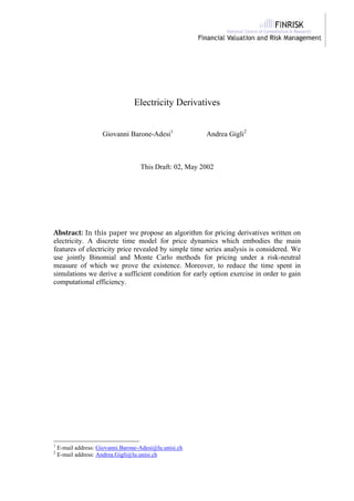
3. 0
40
80
120
160
200
240
280
320
360
99:01 99:07 00:01 00:07 01:01 01:07 02:01
Netherlands market
0
10
20
30
40
50
60
70
80
99:01 99:07 00:01 00:07 01:01 01:07 02:01
NORDPOOL market
Figure 1: Electricity spot prices from Netherland and NordPool markets.
Wt =
½
1 with probability qt
0 with probability 1 ¡ qt
Zt =
½
1 if t = Q(S¿ )
0 otherwise
The function f(Xt; t) may allow for seasonalities in the di¤usion, otherwise we
may choose f(Xt; t) = Xt. The probability qt is the probability that a spike is
realized at time t, provided t > Q(S¿ ). The duration of spike occurred at time
t(i)
, D(St(i) ), is assumed to be independent of spike magnitude and price level.
Equation (1) de…nes changes in electricity prices in an additive way. The
…rst component represents a di¤usion, the second allows for positive percentual
changes when a new spike happens and the third one models the collapsing of
electricity prices when a spike breaks down. The last two components a¤ect
prices only when the indicator functions Wt or Zt are equal to 1. The former
depends on the probability that a spike happens, which we assume to be zero if
the previous spike is still a¤ecting prices, the latter is equal to one only at the
time the previous spike breaks down.
For modeling purposes it is useful to de…ne pt = ¸(t)¢t as the unconditional
probability of spike arrivals in ¢t and to carry out the simulations using this
measure. Indeed, we may simply simulate spikes in t > Q(S¿ ) using pt. Another
advantage of using pt to simulate spike arrivals is that it is easier to include
seasonal dependence and dependence from previous spike realizations in the
spike frequency parameter.
For example, m multiple peridiodicities may be included de…ning the spike
frequency parameter like ¸(t) =
mP
i=1
!i sin
¡
2¼°iti
¢
, where time t is expressed
as a fraction of the year and !i and °i are parameters speci…ed to match peri-
odicities. Alternatively, dependence on the previous n realizations of the pure
spike process can be introduced de…ning ¸(t) = ¸+
nP
k=1
µt
¸(t¡k)I(t¡k), where
0 < µ < 1 and I(j ¡ k) is an indicator function which takes value 1 if a spike
has happened at time t ¡ k, and zero otherwise.
3

4. Another possible extension of our formulation regards the way the electricity
price reverts to the di¤usion process. If we call t(i)
the time of the i-th spike, it
would be not di¢cult to model the decline of the electricity price over the period
D(St(i) ) on a smoothed fashion rather than considering an istantaneous adjust-
ment toward the di¤usion process after Q(St(i) ). Anyway, in the remaining of
this paper we consider the simplest case, with pt = ¸¢t.
3 Derivative Pricing
In this section we show how it is possible to implement an algorithm that is
consistent with the model described in the previous section. The pricing of
contracts such as Forwards or Swaps is not very complicate given that we can
express the price in T of the former under a risk-adjusted measure as
FT = E
£
E(N¡1)¢t + ¢f(XN¢t; N¢t) + WN¢tSN¢tE(N¡1)¢t ¡ ZN¢tS¿ E(N¡1)¢t
¤
where T = N¢t. The price of the latter in 0 is
SW0 =
MX
i=1
(FTi ¡ L)e¡riTi
where ri is the discount rate for maturity Ti and L is the …xed price observed at
the inception of the swap. The current …xed price for maturity M is determined
solving SW0 = 0.
The pricing of options is not immediate and in the remaining of this section
we will show how to implement our model for them. We de…ne options as rights
to either buy or sell a given quantity of energy at the current spot price.
On the basis of the previous considerations and for the sake of clearness we
list below the speci…c assumptions used during the implementation.
² The distribution of the spike sizes follows a lognormal distribution. We
assume that the spiky behavior in electricity prices is governed by a ran-
dom positive percentage variation in the level of the di¤usion process with
mode SM and variance 0:04.
² Spikes happen ad random times but they cannot cumulate. We generate
spikes as realizations of a random processes driven by pt’s but we put
some constraints to get a simulation under qt’s. For example, considering
a binomial tree with period ¢t, number of levels N = T=¢t, we may use
the condition that draws from the uniform distribution over the interval
(0; 1) be smaller than ¸¢t to simulate N realizations of the variable It,
taking value 1 if a spike happens and zero otherwise. Here ¸ serves as
spike frequency, that is the expected number of spikes in a year under
pt’s. In practice, simulation under qt’s is possible imposing that a non-
zero realization of It be considered as a realization of a spike only if it
happens after the previous spike is broken down.
² Spike duration is independent of spike frequency. We use an exponential
random variable with parameter µ to draw spike durations, D(St). We set
time in terms of years, i.e. µ = 0:01 implies an expected duration of the
spike is about 3 days.
4

5. The pricing is based on a three-step procedure. Let ¢t = T=N, where N is
the number of intervals in which we discretize the time to maturity T:
1. In the …rst step we build a tree based on the di¤usion process with pa-
rameter ¹ and ¾;
2. In the second we simulate 1,000 pathways. Each pathway includes N spike
realizations along the tree according to
It =
½
1 if ut < ¸ £ ¢t
0 otherwise
where ut » U(0; 1). For each time interval in which a spike arrives we
draw the percentage change in Xt, St, from a lognormal distribution with
mode SM and variance 0:04. At the same time the duration of each spike
occurrence is drawn from an exponential distribution with parameter µ.
The process with spikes is obtained multiplying the nodes of the tree from
t(i)
to T(St(i) ) by 1+St(i) for the i-th spike, being careful to avoid multiple
spikes in the same periods. An example is shown in …gure (2).
3. The last step requires the computation of the option price along each of
the 1,000 trees.We then take their mean as a way to integrate over the
di¤erent spike process realizations.
European options prices are in‡uenced by the spike e¤ect only if a spike
arrives or is not yet broken down in the last period. The prices on each tree can
be computed by the binomial method as the discounted option payo¤s weighted
for the risk neutral probabilities, given the strike price K. The average price
across trees is the option price.
The American option case is computationally more intensive because it re-
quire to go forward and backward along 1,000 trees. To speed up the option
valuation procedure a su¢cient condition for option exercise can be used. In
fact it can be shown that if
Ete¡¾
p
¢t(N¢t¡t)
¡ K > 0 (2)
then it is rational to exercise the American call option in t, provided that no
other spike happens later. Obviously when this condition applies we do not need
to take into account nodes after t. The computational gain is greater especially
if spikes are huge and rare, time to maturity is low and the di¤usion coe¢cient
is small. In the section related to simulation results we show both the pricing
using this condition and the usual binomial tree pricing.
4 Simulation results
Following the model just described we compute American call option prices
assuming that the price of Electricity is 100$ at time 0 and the risk free rate
is 5%. In Table (1) we report American option prices under the usual Black-
Scholes di¤usion model for comparison. In Tables (3) - (14) we have computed
derivative prices considering di¤erent values for the time to maturity (1 year
and 6 months), strike (80, 100, 120), volatility (20% and 35%), spike magnitude
5

6. K = 80 K = 100 K = 120
T = 1:0 ¾ = 0:20 N = 100 20:6834 7:6466 2:0647
T = 1:0 ¾ = 0:20 N = 500 20:6797 7:6594 2:0546
T = 1:0 ¾ = 0:35 N = 100 24:1465 13:3365 7:0071
T = 1:0 ¾ = 0:35 N = 500 24:1413 13:3588 6:9810
T = 0:5 ¾ = 0:20 N = 100 20:1149 5:5126 0:7068
T = 0:5 ¾ = 0:20 N = 500 20:1168 5:5224 0:7046
T = 0:5 ¾ = 0:35 N = 100 21:8756 9:6306 3:5556
T = 0:5 ¾ = 0:35 N = 500 21:8630 9:6478 3:5445
Table 1: American call option prices obtained by standard binomial pricing for
some values of T, ¾, N and K. The starting value of the underlying price is 100
and it is assumed to follow a simple di¤usion.
(lognormal mode equal to 10% and 50%), frequency (1 and 3 expected number
of spikes each year) and duration (0.01 and 0.03 years). The last three columns
of the tables shows the call price computed using the su¢cient condition, C0, the
usual backward recursion on the binomial tree, C0 and a linear approximation
C¤
0 .
The number of periods in which we have divided the time to maturity is not
really important for pricing. In practice what really matter about the choice
of time steps is to avoid that several spikes with duration lower then ¢t be
excluded while valuation is carried out. In a more general setting, we may set
¢t for each replication only after having determined the shortest duration of
spikes for a given replication.
At …rst look, prices obtained under our model are much higher then those
reported in Table (1). The di¤erence is due to the inclusion of the spike process
and the di¤erences are particularly sensible to the degree of moneyness, time to
maturity, ¸ and SM . The di¤usion coe¢cient ¾ has little importance because
the risk it represents is overwhelmed by those implied by the spiky behavior of
the electricity prices.
Considering the prices obtained including the condition in Equation (2) it
appears that these are close to C0 when we refer to in-the-money options and
the bias increases as long as moneyness decreases, reaching the highest level
when we are pricing out-of-the-money options, spikes are big and relatively
frequent (¸ = 3). In these cases C0 is however signi…cantly greater than the
corresponding European value in Table (1) because of the possibility of spikes
occurring before the last period. That is di¤erent from the classical result in
…nancial markets, that out-of-the money American options have values close to
corresponding European options.
In the tables reporting pricing results there is evidence that the strategy
implied in Equation (2) sometimes leads to a signi…cant loss of value on early
exercise. Therefore Equation (2) is not always adequate for pricing options and
we need to correct the price in these cases. We have seen that our approximation
performs very well when T, ¸ and SM are small. In order to …nd a correction
for this bias in all the other cases and maintaining the gain in computational
e¢ciency using (2), we have expressed the bias standardized by the strike price
as a function of the spike intensity, the product of the frequency parameter and
6

7. t ¡ Statistic P ¡ values
^¯1 0:016370 0:004893 0:00111
^¯2 0:023631 0:000529 2:96E ¡ 45
^¯3 ¡0:018936 0:003423 5:65E ¡ 13
R2
95%
F ¡ statistic 1022:514 0:000000
AIC ¡5:780151
Table 2: Estimation result from model (3).
time to maturity and the moneyness degree. The simple linear model
µ
C0 ¡ C0
K
¶
i
= ¯1SM;i + ¯2Ti¸i + ¯3
µ
E0
K
¶
i
+ ui (3)
has been estimated for pricing settings with SM ¸ 0:5 and N = 100. Results in
Table (2) show that this simple speci…cation explains well the bias and it has
the feature to be quite general to avoid over…tting, which is crucial to …nd a
good correction. Now, using
C¤
0 = C0 + K
µ
^¯1SM + ^¯2T¸ + ^¯3
E0
K
¶
(4)
we have corrected C0 and obtained interesting results for several combina-
tions of the parameters1
. The Mean Absolute Error is 1:19$ when SM = 0:5
and 1:21$ when SM = 1 against 4:71$ and 6:26$ obtained without using the cor-
rection2
. The highest errors (4$) occur when spikes are very frequent (¸ = 5).
In our opinion this residual bias is due to the linear form of the correction in
(4). The complete backward recursion should be used in these cases. Detailed
results are shown in Tables (3) - (14).
5 Concluding Remarks
We present a procedure to price derivatives written on electricity. The appli-
cation proposed in detail is the pricing of American call options, assuming a
constant spike frequency, lognormally distributed spike magnitude and expo-
nentially distributed spike durations. The model can be generalized considering
time dependent parameters and include seasonalities and even multiple period-
icities as we have exempli…ed for ¸.
Simulations results have shown that prices obtained under our algorithm are
very di¤erent from those obtained by standard option pricing models. Moreover
using the condition in Equation (2) the time spent in computations can be
reduced. This condition works almost perfectly if no other spike occurs after
1 In testing the correction we have considered combinations of the following parameters:
¸ = 0:5; 1; 3; 5, T = 0:25; 0:5; 1; 1:5, SM = 0:5; 1,and K = 100; 105; 115; 120
2 We have we have not considered in-the-money options because their inclusion would have
biased toward zero the MAE estimate.
7

8. ITM SM = 0:1 C0 C0 C¤
0
T = 0:5 µ = 0:01 ¸ = 1 ¾ = 0:20 N = 100 29:8750 29:9848 29:0576
T = 0:5 µ = 0:01 ¸ = 1 ¾ = 0:20 N = 500 29:5986 29:7658 28:7812
T = 0:5 µ = 0:01 ¸ = 1 ¾ = 0:35 N = 100 30:5422 30:7317 29:7248
T = 0:5 µ = 0:01 ¸ = 1 ¾ = 0:35 N = 500 30:1514 30:3610 29:3340
T = 0:5 µ = 0:01 ¸ = 3 ¾ = 0:20 N = 100 37:6916 38:3850 38:7647
T = 0:5 µ = 0:01 ¸ = 3 ¾ = 0:20 N = 500 36:9241 38:0500 37:9972
T = 0:5 µ = 0:01 ¸ = 3 ¾ = 0:35 N = 100 37:8888 38:9504 38:9619
T = 0:5 µ = 0:01 ¸ = 3 ¾ = 0:35 N = 500 37:7231 38:9613 38:7962
T = 0:5 µ = 0:03 ¸ = 1 ¾ = 0:20 N = 100 29:5485 29:6705 28:7311
T = 0:5 µ = 0:03 ¸ = 1 ¾ = 0:20 N = 500 29:9932 30:1945 29:1758
T = 0:5 µ = 0:03 ¸ = 1 ¾ = 0:35 N = 100 30:5383 30:6589 29:7209
T = 0:5 µ = 0:03 ¸ = 1 ¾ = 0:35 N = 500 30:2876 30:5165 29:4702
T = 0:5 µ = 0:03 ¸ = 3 ¾ = 0:20 N = 100 37:7446 38:3995 38:8177
T = 0:5 µ = 0:03 ¸ = 3 ¾ = 0:20 N = 500 37:1316 38:1575 38:2047
T = 0:5 µ = 0:03 ¸ = 3 ¾ = 0:35 N = 100 37:8791 38:8375 38:9522
T = 0:5 µ = 0:03 ¸ = 3 ¾ = 0:35 N = 500 37:0842 38:2996 38:1573
Table 3: American call option prices obtained by the algorithm using 1,000
realizations of a spike process for some values of T, µ, ¸, ¾, N. The mode of
the distribution of spike intensities is SM and the strike is 80.
ITM SM = 0:1 C0 C0 C¤
0
T = 1:0 µ = 0:01 ¸ = 1 ¾ = 0:20 N = 100 36:1214 36:7029 36:2492
T = 1:0 µ = 0:01 ¸ = 1 ¾ = 0:20 N = 500 36:2104 36:8911 36:3382
T = 1:0 µ = 0:01 ¸ = 1 ¾ = 0:35 N = 100 37:2837 38:1680 37:4115
T = 1:0 µ = 0:01 ¸ = 1 ¾ = 0:35 N = 500 37:2801 38:2733 37:4079
T = 1:0 µ = 0:01 ¸ = 3 ¾ = 0:20 N = 100 42:3448 44:6130 46:2536
T = 1:0 µ = 0:01 ¸ = 3 ¾ = 0:20 N = 500 41:4840 44:7876 45:3928
T = 1:0 µ = 0:01 ¸ = 3 ¾ = 0:35 N = 100 42:1189 45:3512 46:0277
T = 1:0 µ = 0:01 ¸ = 3 ¾ = 0:35 N = 500 41:3902 45:5511 45:2990
T = 1:0 µ = 0:03 ¸ = 1 ¾ = 0:20 N = 100 36:0188 36:5551 36:1466
T = 1:0 µ = 0:03 ¸ = 1 ¾ = 0:20 N = 500 35:3979 36:1548 35:5257
T = 1:0 µ = 0:03 ¸ = 1 ¾ = 0:35 N = 100 36:8613 37:7634 36:9891
T = 1:0 µ = 0:03 ¸ = 1 ¾ = 0:35 N = 500 37:2322 38:2289 37:3600
T = 1:0 µ = 0:03 ¸ = 3 ¾ = 0:20 N = 100 42:1325 44:5772 46:0413
T = 1:0 µ = 0:03 ¸ = 3 ¾ = 0:20 N = 500 41:3921 44:4825 45:3009
T = 1:0 µ = 0:03 ¸ = 3 ¾ = 0:35 N = 100 42:0098 45:2732 45:9186
T = 1:0 µ = 0:03 ¸ = 3 ¾ = 0:35 N = 500 41:0580 45:2355 44:9668
Table 4: American call option prices obtained by the algorithm using 1,000
realizations of a spike process for some values of T, µ, ¸, ¾, N. The mode of
the distribution of spike intensities is SM and the strike is 80.
8

9. ITM SM = 0:5 C0 C0 C¤
0
T = 0:5 µ = 0:01 ¸ = 1 ¾ = 0:20 N = 100 46:3913 46:4801 46:0977
T = 0:5 µ = 0:01 ¸ = 1 ¾ = 0:20 N = 500 46:5027 46:9213 46:2091
T = 0:5 µ = 0:01 ¸ = 1 ¾ = 0:35 N = 100 46:8861 47:2384 46:5925
T = 0:5 µ = 0:01 ¸ = 1 ¾ = 0:35 N = 500 47:3166 47:9577 47:0230
T = 0:5 µ = 0:01 ¸ = 3 ¾ = 0:20 N = 100 71:5896 72:7866 73:1865
T = 0:5 µ = 0:01 ¸ = 3 ¾ = 0:20 N = 500 71:0383 73:5544 72:6352
T = 0:5 µ = 0:01 ¸ = 3 ¾ = 0:35 N = 100 71:3235 73:7031 72:9204
T = 0:5 µ = 0:01 ¸ = 3 ¾ = 0:35 N = 500 70:5442 73:9954 72:1411
T = 0:5 µ = 0:03 ¸ = 1 ¾ = 0:20 N = 100 45:7253 45:9190 45:4317
T = 0:5 µ = 0:03 ¸ = 1 ¾ = 0:20 N = 500 46:6874 47:0690 46:3938
T = 0:5 µ = 0:03 ¸ = 1 ¾ = 0:35 N = 100 47:2720 47:5610 46:9784
T = 0:5 µ = 0:03 ¸ = 1 ¾ = 0:35 N = 500 46:6034 47:2365 46:3098
T = 0:5 µ = 0:03 ¸ = 3 ¾ = 0:20 N = 100 73:7413 74:6968 75:3382
T = 0:5 µ = 0:03 ¸ = 3 ¾ = 0:20 N = 500 71:0943 73:3377 72:6912
T = 0:5 µ = 0:03 ¸ = 3 ¾ = 0:35 N = 100 71:5541 73:1945 73:1510
T = 0:5 µ = 0:03 ¸ = 3 ¾ = 0:35 N = 500 70:1634 73:0487 71:7603
Table 5: American call option prices obtained by the algorithm using 1,000
realizations of a spike process for some values of T, µ, ¸, ¾, N. The mode of
the distribution of spike intensities is SM and the strike is 80.
ITM SM = 0:5 C0 C0 C¤
0
T = 1:0 µ = 0:01 ¸ = 1 ¾ = 0:20 N = 100 62:5343 63:5429 63:1860
T = 1:0 µ = 0:01 ¸ = 1 ¾ = 0:20 N = 500 62:1316 63:5358 62:7833
T = 1:0 µ = 0:01 ¸ = 1 ¾ = 0:35 N = 100 62:2228 63:8457 62:8745
T = 1:0 µ = 0:01 ¸ = 1 ¾ = 0:35 N = 500 63:7876 65:6090 64:4393
T = 1:0 µ = 0:01 ¸ = 3 ¾ = 0:20 N = 100 84:9457 88:7413 89:3783
T = 1:0 µ = 0:01 ¸ = 3 ¾ = 0:20 N = 500 82:4418 89:0597 86:8744
T = 1:0 µ = 0:01 ¸ = 3 ¾ = 0:35 N = 100 83:5325 89:2921 87:9651
T = 1:0 µ = 0:01 ¸ = 3 ¾ = 0:35 N = 500 81:9741 89:6744 86:4067
T = 1:0 µ = 0:03 ¸ = 1 ¾ = 0:20 N = 100 64:3828 65:4066 65:0345
T = 1:0 µ = 0:03 ¸ = 1 ¾ = 0:20 N = 500 61:3676 63:4218 62:0193
T = 1:0 µ = 0:03 ¸ = 1 ¾ = 0:35 N = 100 62:4802 63:8345 63:1319
T = 1:0 µ = 0:03 ¸ = 1 ¾ = 0:35 N = 500 63:2104 65:3867 63:8621
T = 1:0 µ = 0:03 ¸ = 3 ¾ = 0:20 N = 100 85:6443 89:3603 90:0770
T = 1:0 µ = 0:03 ¸ = 3 ¾ = 0:20 N = 500 83:3663 89:9129 87:7990
T = 1:0 µ = 0:03 ¸ = 3 ¾ = 0:35 N = 100 82:9634 88:9521 87:3960
T = 1:0 µ = 0:03 ¸ = 3 ¾ = 0:35 N = 500 80:6769 89:0712 85:1095
Table 6: American call option prices obtained by the algorithm using 1,000
realizations of a spike process for some values of T, µ, ¸, ¾, N. The mode of
the distribution of spike intensities is SM and the strike is 80.
9

10. ATM SM = 0:1 C0 C0 C¤
0
T = 0:5 µ = 0:01 ¸ = 1 ¾ = 0:20 N = 100 12:9826 13:2223 12:4342
T = 0:5 µ = 0:01 ¸ = 1 ¾ = 0:20 N = 500 13:0809 13:2710 12:5325
T = 0:5 µ = 0:01 ¸ = 1 ¾ = 0:35 N = 100 15:9707 16:2493 15:4223
T = 0:5 µ = 0:01 ¸ = 1 ¾ = 0:35 N = 500 15:5470 15:9175 14:9986
T = 0:5 µ = 0:01 ¸ = 3 ¾ = 0:20 N = 100 18:6140 19:9391 20:4287
T = 0:5 µ = 0:01 ¸ = 3 ¾ = 0:20 N = 500 18:3560 19:7200 20:1707
T = 0:5 µ = 0:01 ¸ = 3 ¾ = 0:35 N = 100 20:1706 21:9318 21:9853
T = 0:5 µ = 0:01 ¸ = 3 ¾ = 0:35 N = 500 19:8078 21:4986 21:6225
T = 0:5 µ = 0:03 ¸ = 1 ¾ = 0:20 N = 100 12:7450 12:9948 12:1966
T = 0:5 µ = 0:03 ¸ = 1 ¾ = 0:20 N = 500 13:0198 13:2713 12:4714
T = 0:5 µ = 0:03 ¸ = 1 ¾ = 0:35 N = 100 15:5891 15:9733 15:0407
T = 0:5 µ = 0:03 ¸ = 1 ¾ = 0:35 N = 500 15:9066 16:3703 15:3582
T = 0:5 µ = 0:03 ¸ = 3 ¾ = 0:20 N = 100 18:5443 19:7896 20:3590
T = 0:5 µ = 0:03 ¸ = 3 ¾ = 0:20 N = 500 18:1380 19:4866 19:9527
T = 0:5 µ = 0:03 ¸ = 3 ¾ = 0:35 N = 100 19:9624 21:7101 21:7771
T = 0:5 µ = 0:03 ¸ = 3 ¾ = 0:35 N = 500 20:0721 21:9510 21:8868
Table 7: American call option prices obtained by the algorithm using 1,000
realizations of a spike process for some values of T, µ, ¸, ¾, N. The mode of
the distribution of spike intensities is SM and the strike is 100.
ATM SM = 0:1 C0 C0 C¤
0
T = 1:0 µ = 0:01 ¸ = 1 ¾ = 0:20 N = 100 18:5186 19:3222 19:1520
T = 1:0 µ = 0:01 ¸ = 1 ¾ = 0:20 N = 500 18:5474 19:4738 19:1806
T = 1:0 µ = 0:01 ¸ = 1 ¾ = 0:35 N = 100 22:0031 23:5042 22:6363
T = 1:0 µ = 0:01 ¸ = 1 ¾ = 0:35 N = 500 21:6968 23:3463 22:3300
T = 1:0 µ = 0:01 ¸ = 3 ¾ = 0:20 N = 100 21:8986 25:8139 27:2580
T = 1:0 µ = 0:01 ¸ = 3 ¾ = 0:20 N = 500 21:6284 25:9550 26:9878
T = 1:0 µ = 0:01 ¸ = 3 ¾ = 0:35 N = 100 23:4219 28:8784 28:7813
T = 1:0 µ = 0:01 ¸ = 3 ¾ = 0:35 N = 500 23:4479 29:0103 28:8073
T = 1:0 µ = 0:03 ¸ = 1 ¾ = 0:20 N = 100 18:6384 19:4981 19:2716
T = 1:0 µ = 0:03 ¸ = 1 ¾ = 0:20 N = 500 18:6182 19:7847 19:2514
T = 1:0 µ = 0:03 ¸ = 1 ¾ = 0:35 N = 100 21:9422 23:4627 22:5754
T = 1:0 µ = 0:03 ¸ = 1 ¾ = 0:35 N = 500 21:4499 23:0300 22:0831
T = 1:0 µ = 0:03 ¸ = 3 ¾ = 0:20 N = 100 22:2485 26:2281 27:6079
T = 1:0 µ = 0:03 ¸ = 3 ¾ = 0:20 N = 500 21:8104 25:7352 27:1698
T = 1:0 µ = 0:03 ¸ = 3 ¾ = 0:35 N = 100 23:7080 29:1479 29:0674
T = 1:0 µ = 0:03 ¸ = 3 ¾ = 0:35 N = 500 23:0125 28:8168 28:3719
Table 8: American call option prices obtained by the algorithm using 1,000
realizations of a spike process for some values of T, µ, ¸, ¾, N. The mode of
the distribution of spike intensities is SM and the strike is 100.
10

11. ATM SM = 0:5 C0 C0 C¤
0
T = 0:5 µ = 0:01 ¸ = 1 ¾ = 0:20 N = 100 29:2419 29:4422 29:3483
T = 0:5 µ = 0:01 ¸ = 1 ¾ = 0:20 N = 500 29:3349 29:8570 29:4413
T = 0:5 µ = 0:01 ¸ = 1 ¾ = 0:35 N = 100 31:2238 31:7673 31:3302
T = 0:5 µ = 0:01 ¸ = 1 ¾ = 0:35 N = 500 31:7474 32:4010 31:8538
T = 0:5 µ = 0:01 ¸ = 3 ¾ = 0:20 N = 100 52:0969 54:0428 54:5664
T = 0:5 µ = 0:01 ¸ = 3 ¾ = 0:20 N = 500 51:5843 54:7923 54:0538
T = 0:5 µ = 0:01 ¸ = 3 ¾ = 0:35 N = 100 52:5536 55:5433 55:0231
T = 0:5 µ = 0:01 ¸ = 3 ¾ = 0:35 N = 500 52:0156 55:8333 54:4851
T = 0:5 µ = 0:03 ¸ = 1 ¾ = 0:20 N = 100 28:6794 28:9403 28:7858
T = 0:5 µ = 0:03 ¸ = 1 ¾ = 0:20 N = 500 29:5670 29:9929 29:6734
T = 0:5 µ = 0:03 ¸ = 1 ¾ = 0:35 N = 100 31:5247 32:0603 31:6311
T = 0:5 µ = 0:03 ¸ = 1 ¾ = 0:35 N = 500 31:1372 31:8324 31:2436
T = 0:5 µ = 0:03 ¸ = 3 ¾ = 0:20 N = 100 54:1376 55:8021 56:6071
T = 0:5 µ = 0:03 ¸ = 3 ¾ = 0:20 N = 500 51:8601 54:5755 54:3296
T = 0:5 µ = 0:03 ¸ = 3 ¾ = 0:35 N = 100 52:8258 55:0459 55:2953
T = 0:5 µ = 0:03 ¸ = 3 ¾ = 0:35 N = 500 51:5920 54:9025 54:0615
Table 9: American call option prices obtained by the algorithm using 1,000
realizations of a spike process for some values of T, µ, ¸, ¾, N. The mode of
the distribution of spike intensities is SM and the strike is 100.
ATM SM = 0:5 C0 C0 C¤
0
T = 1:0 µ = 0:01 ¸ = 1 ¾ = 0:20 N = 100 44:6127 46:0056 45:9007
T = 1:0 µ = 0:01 ¸ = 1 ¾ = 0:20 N = 500 44:3551 46:0665 45:6431
T = 1:0 µ = 0:01 ¸ = 1 ¾ = 0:35 N = 100 45:8577 47:6927 47:1457
T = 1:0 µ = 0:01 ¸ = 1 ¾ = 0:35 N = 500 47:0810 49:1886 48:3690
T = 1:0 µ = 0:01 ¸ = 3 ¾ = 0:20 N = 100 64:4447 69:5363 70:4589
T = 1:0 µ = 0:01 ¸ = 3 ¾ = 0:20 N = 500 62:1149 69:8241 68:1291
T = 1:0 µ = 0:01 ¸ = 3 ¾ = 0:35 N = 100 63:4817 70:4774 69:4959
T = 1:0 µ = 0:01 ¸ = 3 ¾ = 0:35 N = 500 62:4178 70:8811 68:4320
T = 1:0 µ = 0:03 ¸ = 1 ¾ = 0:20 N = 100 46:3017 47:7776 47:5897
T = 1:0 µ = 0:03 ¸ = 1 ¾ = 0:20 N = 500 43:6654 45:9829 44:9534
T = 1:0 µ = 0:03 ¸ = 1 ¾ = 0:35 N = 100 45:9468 47:6148 47:2348
T = 1:0 µ = 0:03 ¸ = 1 ¾ = 0:35 N = 500 46:6011 48:9510 47:8891
T = 1:0 µ = 0:03 ¸ = 3 ¾ = 0:20 N = 100 64:3964 70:1050 70:4106
T = 1:0 µ = 0:03 ¸ = 3 ¾ = 0:20 N = 500 62:9806 70:6535 68:9948
T = 1:0 µ = 0:03 ¸ = 3 ¾ = 0:35 N = 100 62:7815 70:2011 68:7957
T = 1:0 µ = 0:03 ¸ = 3 ¾ = 0:35 N = 500 61:0449 70:3456 67:0591
Table 10: American call option prices obtained by the algorithm using 1,000
realizations of a spike process for some values of T, µ, ¸, ¾, N. The mode of
the distribution of spike intensities is SM and the strike is 100.
11

12. OTM SM = 0:1 C0 C0 C¤
0
T = 0:5 µ = 0:01 ¸ = 1 ¾ = 0:20 N = 100 2:7645 3:1451 2:4852
T = 0:5 µ = 0:01 ¸ = 1 ¾ = 0:20 N = 500 2:7800 3:1604 2:5007
T = 0:5 µ = 0:01 ¸ = 1 ¾ = 0:35 N = 100 6:0904 6:6743 5:8111
T = 0:5 µ = 0:01 ¸ = 1 ¾ = 0:35 N = 500 5:9745 6:6759 5:6952
T = 0:5 µ = 0:01 ¸ = 3 ¾ = 0:20 N = 100 4:1711 5:9766 6:7275
T = 0:5 µ = 0:01 ¸ = 3 ¾ = 0:20 N = 500 4:2016 6:0476 6:7580
T = 0:5 µ = 0:01 ¸ = 3 ¾ = 0:35 N = 100 7:0232 9:7962 9:5796
T = 0:5 µ = 0:01 ¸ = 3 ¾ = 0:35 N = 500 7:1634 9:8647 9:7198
T = 0:5 µ = 0:03 ¸ = 1 ¾ = 0:20 N = 100 2:8829 3:2678 2:6036
T = 0:5 µ = 0:03 ¸ = 1 ¾ = 0:20 N = 500 2:8327 3:2921 2:5534
T = 0:5 µ = 0:03 ¸ = 1 ¾ = 0:35 N = 100 6:0658 6:8635 5:7865
T = 0:5 µ = 0:03 ¸ = 1 ¾ = 0:35 N = 500 6:2296 6:9138 5:9503
T = 0:5 µ = 0:03 ¸ = 3 ¾ = 0:20 N = 100 4:2663 6:1963 6:8227
T = 0:5 µ = 0:03 ¸ = 3 ¾ = 0:20 N = 500 4:2507 6:2362 6:8071
T = 0:5 µ = 0:03 ¸ = 3 ¾ = 0:35 N = 100 7:2157 9:9773 9:7721
T = 0:5 µ = 0:03 ¸ = 3 ¾ = 0:35 N = 500 6:9814 9:8383 9:5378
Table 11: American call option prices obtained by the algorithm using 1,000
realizations of a spike process for some values of T, µ, ¸, ¾, N. The mode of
the distribution of spike intensities is SM and the strike is 120.
OTM SM = 0:1 C0 C0 C¤
0
T = 1:0 µ = 0:01 ¸ = 1 ¾ = 0:20 N = 100 5:8406 7:3510 6:9792
T = 1:0 µ = 0:01 ¸ = 1 ¾ = 0:20 N = 500 6:1324 7:5509 7:2710
T = 1:0 µ = 0:01 ¸ = 1 ¾ = 0:35 N = 100 10:6793 13:0845 11:8179
T = 1:0 µ = 0:01 ¸ = 1 ¾ = 0:35 N = 500 10:7492 13:0215 11:8878
T = 1:0 µ = 0:01 ¸ = 3 ¾ = 0:20 N = 100 5:9835 11:3237 12:7935
T = 1:0 µ = 0:01 ¸ = 3 ¾ = 0:20 N = 500 5:9308 11:0995 12:7408
T = 1:0 µ = 0:01 ¸ = 3 ¾ = 0:35 N = 100 9:4740 17:2252 16:2840
T = 1:0 µ = 0:01 ¸ = 3 ¾ = 0:35 N = 500 9:3099 17:0246 16:1199
T = 1:0 µ = 0:03 ¸ = 1 ¾ = 0:20 N = 100 6:1037 7:6047 7:2422
T = 1:0 µ = 0:03 ¸ = 1 ¾ = 0:20 N = 500 5:7246 7:4503 6:8631
T = 1:0 µ = 0:03 ¸ = 1 ¾ = 0:35 N = 100 10:7727 13:1104 11:9113
T = 1:0 µ = 0:03 ¸ = 1 ¾ = 0:35 N = 500 10:5357 13:3294 11:6743
T = 1:0 µ = 0:03 ¸ = 3 ¾ = 0:20 N = 100 5:9233 11:3846 12:7333
T = 1:0 µ = 0:03 ¸ = 3 ¾ = 0:20 N = 500 5:9878 11:3433 12:7978
T = 1:0 µ = 0:03 ¸ = 3 ¾ = 0:35 N = 100 9:3918 17:3599 16:2018
T = 1:0 µ = 0:03 ¸ = 3 ¾ = 0:35 N = 500 9:1443 17:2594 15:9543
Table 12: American call option prices obtained by the algorithm using 1,000
realizations of a spike process for some values of T, µ, ¸, ¾, N. The mode of
the distribution of spike intensities is SM and the strike is 120.
12

13. OTM SM = 0:5 C0 C0 C¤
0
T = 0:5 µ = 0:01 ¸ = 1 ¾ = 0:20 N = 100 17:6710 18:2194 18:1775
T = 0:5 µ = 0:01 ¸ = 1 ¾ = 0:20 N = 500 18:1478 18:7939 18:6545
T = 0:5 µ = 0:01 ¸ = 1 ¾ = 0:35 N = 100 19:7224 20:3172 20:2289
T = 0:5 µ = 0:01 ¸ = 1 ¾ = 0:35 N = 500 19:9204 20:7207 20:4269
T = 0:5 µ = 0:01 ¸ = 3 ¾ = 0:20 N = 100 34:6956 37:3718 38:0378
T = 0:5 µ = 0:01 ¸ = 3 ¾ = 0:20 N = 500 34:2901 38:0985 37:6323
T = 0:5 µ = 0:01 ¸ = 3 ¾ = 0:35 N = 100 35:2587 38:6438 38:6009
T = 0:5 µ = 0:01 ¸ = 3 ¾ = 0:35 N = 500 35:0963 38:8652 38:4385
T = 0:5 µ = 0:03 ¸ = 1 ¾ = 0:20 N = 100 17:8595 18:3396 18:3660
T = 0:5 µ = 0:03 ¸ = 1 ¾ = 0:20 N = 500 17:9709 18:4808 18:4774
T = 0:5 µ = 0:03 ¸ = 1 ¾ = 0:35 N = 100 19:8336 20:6625 20:3401
T = 0:5 µ = 0:03 ¸ = 1 ¾ = 0:35 N = 500 19:6689 20:4965 20:1754
T = 0:5 µ = 0:03 ¸ = 3 ¾ = 0:20 N = 100 35:1103 37:9307 38:4525
T = 0:5 µ = 0:03 ¸ = 3 ¾ = 0:20 N = 500 34:9616 38:3003 38:3038
T = 0:5 µ = 0:03 ¸ = 3 ¾ = 0:35 N = 100 35:0757 38:2893 38:4179
T = 0:5 µ = 0:03 ¸ = 3 ¾ = 0:35 N = 500 35:1366 38:8880 38:4788
Table 13: American call option prices obtained by the algorithm using 1,000
realizations of a spike process for some values of T, µ, ¸, ¾, N. The mode of
the distribution of spike intensities is SM and the strike is 120.
OTM SM = 0:5 C0 C0 C¤
0
T = 1:0 µ = 0:01 ¸ = 1 ¾ = 0:20 N = 100 29:7326 31:5437 31:6569
T = 1:0 µ = 0:01 ¸ = 1 ¾ = 0:20 N = 500 29:0364 31:1717 30:9607
T = 1:0 µ = 0:01 ¸ = 1 ¾ = 0:35 N = 100 32:2088 34:4994 34:1331
T = 1:0 µ = 0:01 ¸ = 1 ¾ = 0:35 N = 500 32:1511 34:3449 34:0754
T = 1:0 µ = 0:01 ¸ = 3 ¾ = 0:20 N = 100 44:4208 51:3083 52:0166
T = 1:0 µ = 0:01 ¸ = 3 ¾ = 0:20 N = 500 42:3072 51:2874 49:9030
T = 1:0 µ = 0:01 ¸ = 3 ¾ = 0:35 N = 100 43:8272 53:1472 51:4230
T = 1:0 µ = 0:01 ¸ = 3 ¾ = 0:35 N = 500 42:9827 52:8007 50:5785
T = 1:0 µ = 0:03 ¸ = 1 ¾ = 0:20 N = 100 30:5809 32:4505 32:5052
T = 1:0 µ = 0:03 ¸ = 1 ¾ = 0:20 N = 500 29:4335 31:3746 31:3578
T = 1:0 µ = 0:03 ¸ = 1 ¾ = 0:35 N = 100 32:1465 34:1942 34:0708
T = 1:0 µ = 0:03 ¸ = 1 ¾ = 0:35 N = 500 32:4565 35:1242 34:3808
T = 1:0 µ = 0:03 ¸ = 3 ¾ = 0:20 N = 100 43:6222 51:7772 51:2180
T = 1:0 µ = 0:03 ¸ = 3 ¾ = 0:20 N = 500 42:4879 51:3064 50:0837
T = 1:0 µ = 0:03 ¸ = 3 ¾ = 0:35 N = 100 43:2047 51:8437 50:8005
T = 1:0 µ = 0:03 ¸ = 3 ¾ = 0:35 N = 500 42:5801 52:9565 50:1759
Table 14: American call option prices obtained by the algorithm using 1,000
realizations of a spike process for some values of T, µ, ¸, ¾, N. The mode of
the distribution of spike intensities is SM and the strike is 120.
13

14. the time of exercise. In practice we cannot forecast if the spike which veri…es
Equation (2) is really the last one before the maturity. Therefore we need to
correct prices obtained under this condition using Equation (4) when spikes are
frequent, their intensity is high and option time to maturity is long. However
prices from model (1) still remain valid and further studies should be addressed
toward improving computational aspects.
It is clear from the results that the most relevant determinants of the option
price level are the parameters of the spike process. It would be useful to enrich
the model in this direction, adding seasonalities and stylized facts to this compo-
nent. Moreover, our pricing models have been computed under the risk-neutral
measure. The existence of this measure is discussed in the appendix but the
relationship between the physical and the risk-neutral measures is an important
topic for future research. We believe that spike risk is largely idiosyncratic and
this justi…es the binomial pricing method as advocated by Merton (Merton R.,
1992), but only long series of market data may cast light on this issue.
6 Appendix
Let F be the forward price for delivery at T, where T is any relevant time.
De…ne F¤
as the forward price of a contract that delivers electricity if no spike
is in progress at T. If a spike is in progress F¤
delivers against an additional
payment equal to the spike intensity3
. Let M be the expected intensity of the
spike at T. De…ne
¼ =
(F ¡ F¤
)
M
then a risk-neutral measure exists if and only if 0 < ¼ < 1.
PROOF: From the de…nition of ¼.
F¤
= ¼M + (1 ¡ ¼)0 +
Z
Xd eP
where X is the spot price at time T and eP is the risk neutral measure for the
di¤usion process without spikes.
3 Capped forwards, traded in the United States, have prices similar to F¤.
14

15. SM = 0:1 SM = 0:5
K = 120 K = 100 K = 120 K = 100
T = 0:5 µ = 0:01 ¸ = 1 ¾ = 0:20 1:1375 7:0594 1:9645 7:3608
T = 0:5 µ = 0:01 ¸ = 1 ¾ = 0:35 4:3546 11:2197 4:7711 11:4557
T = 0:5 µ = 0:01 ¸ = 3 ¾ = 0:20 1:3416 7:3741 2:3670 8:1194
T = 0:5 µ = 0:01 ¸ = 3 ¾ = 0:35 4:5267 11:6207 5:4795 12:8859
T = 0:5 µ = 0:03 ¸ = 1 ¾ = 0:20 1:2208 7:4976 2:0696 8:8299
T = 0:5 µ = 0:03 ¸ = 1 ¾ = 0:35 4:6356 11:5720 5:4623 12:6670
T = 0:5 µ = 0:03 ¸ = 3 ¾ = 0:20 1:6977 8:1432 4:9431 11:9138
T = 0:5 µ = 0:03 ¸ = 3 ¾ = 0:35 4:9571 12:0864 7:9667 15:0492
T = 1:0 µ = 0:01 ¸ = 1 ¾ = 0:20 3:3493 10:5975 3:7466 11:2411
T = 1:0 µ = 0:01 ¸ = 1 ¾ = 0:35 9:0318 16:2801 9:6239 17:0490
T = 1:0 µ = 0:01 ¸ = 3 ¾ = 0:20 3:6694 11:1631 5:2833 13:1754
T = 1:0 µ = 0:01 ¸ = 3 ¾ = 0:35 9:3584 16:7175 10:6889 17:9083
T = 1:0 µ = 0:03 ¸ = 1 ¾ = 0:20 3:6148 11:0441 5:0901 12:4233
T = 1:0 µ = 0:03 ¸ = 1 ¾ = 0:35 9:2296 16:5490 10:6972 17:9176
T = 1:0 µ = 0:03 ¸ = 3 ¾ = 0:20 4:0952 11:6818 7:8177 14:4743
T = 1:0 µ = 0:03 ¸ = 3 ¾ = 0:35 9:6601 17:4878 12:6447 20:9894
Table 15: European call option prices obtained by the algorithm using 1,000
realizations of a spike process for some values of T, µ, ¸, ¾. The mode of the
distribution of spike intensities is SM and N = 100.
7 Bibliography
References
[1] H. Geman and O. Vasiceck (2001) Forward and future contracts on non
storable commodities: the case of electricity, Preprint.
[2] H. Geman and A. Roncoroni (2001) A class of marked point processes for
modeling electricity prices, ESSEC working paper.
[3] L. Julio and E. Schwartz (2002) Electricity prices and power derivatives:
evidence from the Nordic Power Exchange, Review of Derivatives Research
5, 5-50.
[4] R. Merton (1992), Continuous time …nance, Blackwell, Cambridge, USA.
15

16. Figure 2: The …gure show three examples of spike processes realizations over
binomial trees. The number of levels a¤ected by the spike is random, as well as
the intensity of the spike magnitude.
16