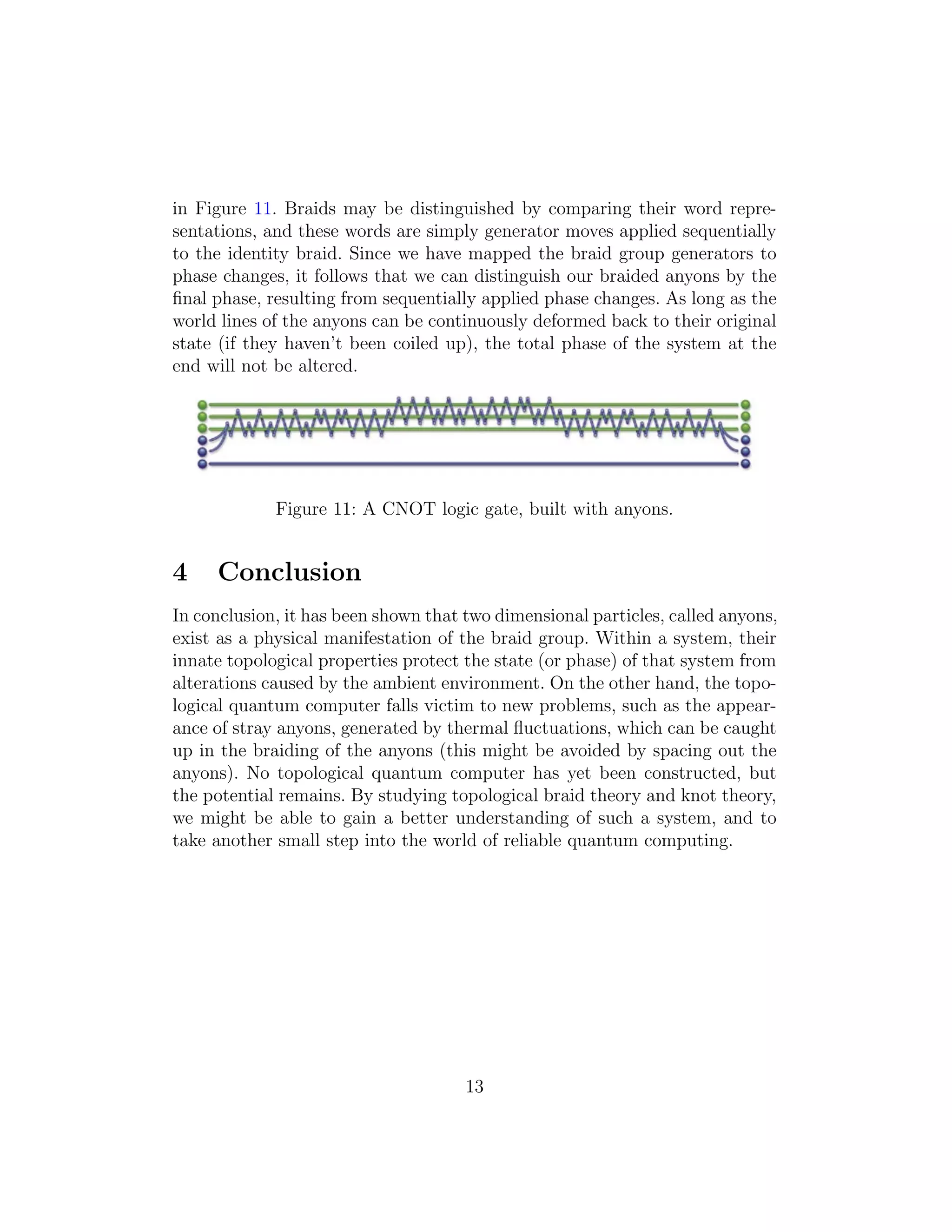
This document provides an overview of topological quantum computing using anyons. It first discusses motivations for alternative computing approaches due to limitations of traditional computing. It then introduces braid theory, including definitions of braids and their equivalence. Braids form a braid group that can represent any braid as a word. Anyons are quasiparticles that emerge in 2D systems and can represent quantum bits in a way that is robust to environmental perturbations. Braids representing the trajectories of anyons over time can encode quantum information and computations in a topological manner.

1. u
Topological Quantum Computing
AN BRIEF OVERVIEW
u
Zach Forster
©December 15, 2015
1

2. Contents
1 Motivations 3
2 Braid Theory 5
2.0.1 What is a Braid? . . . . . . . . . . . . . . . . . . . . . . 5
2.0.2 Equivalence of Braids . . . . . . . . . . . . . . . . . . . 6
2.0.3 The Braid Group . . . . . . . . . . . . . . . . . . . . . . 9
3 Quantum Computing with Anyons 11
4 Conclusion 13
2

3. 1 Motivations
The free lunch is over. This is a sort of slogan which has become quite com-
mon in the world of computing during recent years, but what does it mean?
What it does not mean is that Moore’s Law is dead. It does mean that, to
take advantage of emerging information processing technology, programmers
must learn to be increasingly clever. Hardware designers have been banging
their heads against a few physical “walls” for over a decade now. Heat is-
sues, power constraints, and a shortage of low hanging fruit with respect to
instruction level processing optimizations have stopped the advance of the
single-processor machine dead in its tracks [7].
Figure 1: Processing power no longer increases at the same rate as transistor
count [7].
Designers have since turned to parallel computing in order to maintain the
expected annual exponential increases in processing power. However, due to
the sequential nature of many (perhaps most) programming problems, dou-
bling the number of cores or processors does not double the processing power.
In response, we are seeing the slow death of the personal computer. Many
are investing in massive distributed networks, to which small, lightweight
personal computers can connect and unload most of their work. This is an
interesting reversal of the move from mainframes and timeshare computing
to personal computers in the 1980’s, but it is certainly not an ideal solution.
Many believe that computing power must be kept in the hands of individuals.
3

4. With this in mind, one of the most hyped technologies on the horizon seems
to be quantum computing.
Although some “large” strides (many of which are of debatable significance)
have been made by researchers of quantum computing techniques, many ma-
jor issues continue to persist. One of these is the incredible fragility of a
quantum system. Quantum computers make use of the fact that quantum
bits may hold both of their two possible states simultaneously, with each
state’s complex amplitude expressing its probability of being observed. We
can call these two states 0 and 1, as we do when discussing classical comput-
ing bits. A simpler way of visualizing this is to imagine that a qubit may hold
only one state at each instant, but that that state is a superposition of both 0
and 1. In other words, we can imagine the states as points along the complex
sphere, where the north pole maps to the state 1, the south pole maps to the
state 0, and everything else is a superposition of the two, each weighted by
its amplitude [3]. These superpositions are written as α|0 ą `β|1 ą, where
α and β are complex numbers (the amplitudes of 0 and 1).
Figure 2: A spherical representation of a quantum bit.
The issue is that minute fluctuations in temperature, magnetic field, etc.
can easily disrupt the states of the qubits [3]. This requires incredibly well-
controlled environments to be created, making the personal/portable quan-
tum computer quite impractical. However, a topological approach to quan-
tum computing yields a possible solution.
4

5. 2 Braid Theory
In order to understand how the qubits in a topological quantum computer
can be impervious to environmental perturbations, we must first discuss the
topological structure that they represent. We will therefore give a brief intro-
duction of a subfield of topology called braid theory, a close cousin of knot
theory.
2.0.1 What is a Braid?
One common way to define a braid is by viewing it as a collection of non-
intersecting paths in R3
, each of which connects a point in tpx,0,1q|x P Zu
with a point in tpx,0,0q|x P Zu [4]. Recall that a path from x to y, where
x,y P X is a continuous function f : r0,1s Ñ X, such that fp0q “ x and
fp1q “ y. It may be helpful to point out that, since the paths may not inter-
sect, neither may their endpoints intersect. Figure 3 depicts a braid. Notice
that the endpoints are lined up and evenly spaced, since they are fixed in a
vertical, two-dimensional plane. Conversely, the paths connecting them are
free to travel anywhere in R3
, with two restrictions. First, no point along any
path may have a z-coordinate greater than 1, or less than 0 (i.e. the paths
must stay between the endpoints). Second, the paths must move in the neg-
ative z-direction at all times [1]. Figure 4 shows an example of a braid which
breaks the second rule.
Figure 3: A braid.
5

6. Figure 4: Not a braid.
Instead of imagining braids as a series of paths embedded within R3
, it is
often convenient to project them onto the plane. This is typically done in such
a way as to guarantee that there are finitely many points on the projection
which correspond to two points on the braid, and none which correspond to
more than two points on the braid. This is called a regular projection, and
guarantees that we do not lose information by projecting the braid into a
lower dimensional space [2]. The method of projection is obvious, as we have
already done it by displaying Figure 3 on a two-dimensional sheet of paper.
To project a braid onto the x-z plane, we simply remove the y-coordinate
from every point in path. In order to avoid losing important topological
information, when two paths intersect, we draw the intersection in such a
way that it is obvious which path was at a higher y-value (which path crossed
in front of the other).
Of course, one might imagine that two paths could run for a while with
the same position in the x-z plane (the y-values must differ), so that one
would be hidden behind the other after projection, thus violating our rules.
It turns out that we can always manipulate our paths in such a way that,
after projection, they only intersect at a finite number of points, and that at
most two paths intersect at any point. This deformation does not change the
braid topologically, which brings us to our next section.
2.0.2 Equivalence of Braids
Topological spaces are identified, not by any specific representation, nor by
their appearance when viewed by any specific perspective. Instead, they are
identified by a special topological properties which are preserved by home-
omorphisms. Such topological properties are aptly named invariants [2]. We
give an example with knots before discussing braids, so as to form a connec-
tion with a more familiar subject. The connections will continue to emerge
as we discuss ambient isotopies and words. Such connections arise because
every knot is actually the closure of some braid, formed by connecting the
endpoints of the braid as shown in Figure 5.
6

7. Figure 5: A Knot as the Closure of a Braid.
Imagine knotting up a piece of string, and then fusing the ends together.
Invariants between knots may be (extremely) loosely defined as loops, coils,
ties, etc. which cannot be removed from the knot without cutting it at some
point, unraveling it, and gluing the severed ends back together. Any features
of a knot which are not invariants, may be removed from the knot, so that two
knots with the same invariant features, but with any number of non-invariant
features, may be uncoiled back into identical states. These knots would then
be considered equivalent. Figure 6 shows two such equivalent knots.
Figure 6: Equivalent Knots.
Braids, being very closely related to knots, have a very similar equivalence
relation. Here, it helps to imagine that your braid consists of a series of
strings, tied to two boards. The endpoints of the strings cannot move and
you cannot spin the boards around, but you can otherwise wiggle the strings
around to your heart’s content without changing the identity of the braid.
Figure 7 shows pairs of equivalent braids.
7

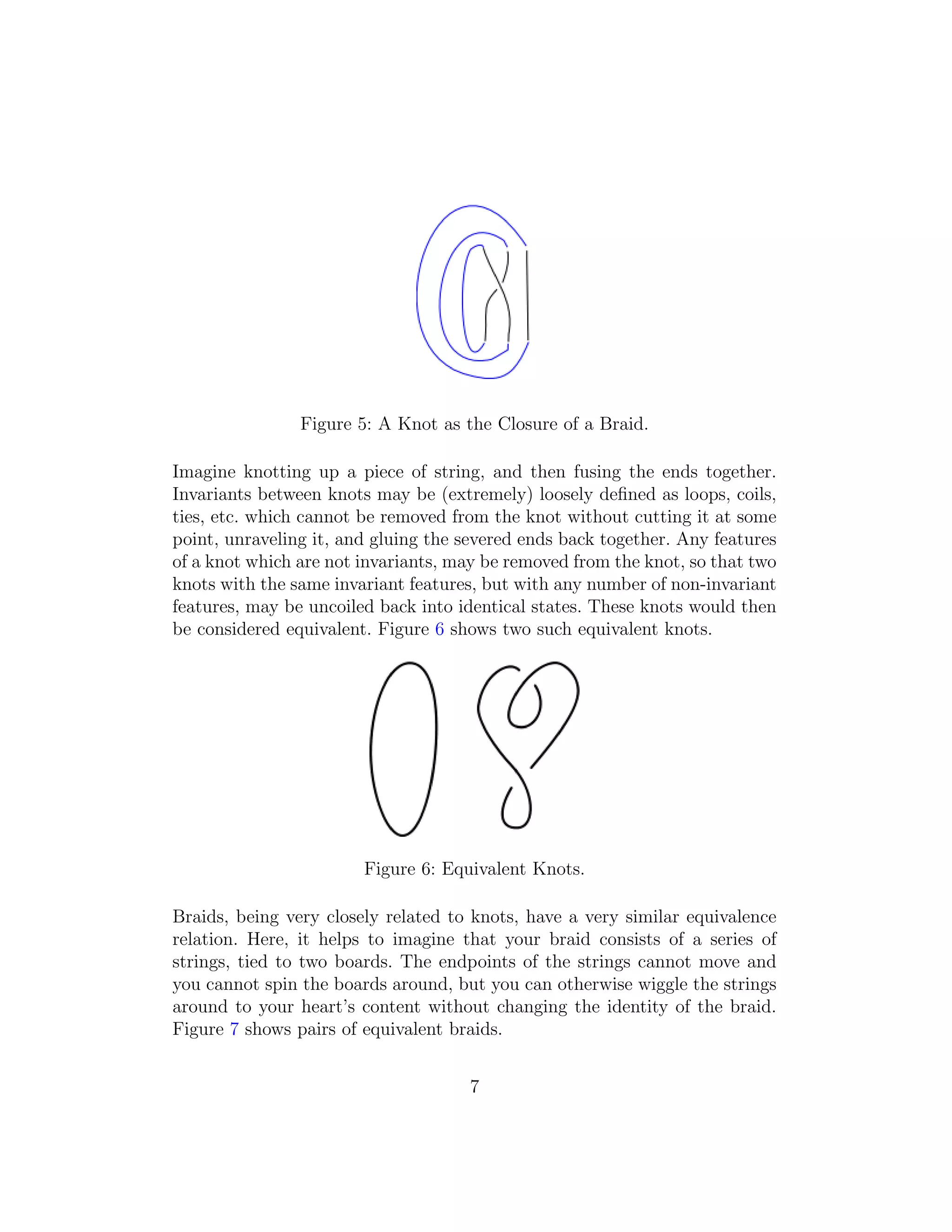
8. Figure 7: Equivalent Braids.
A much more formal definition of this equivalence relation is that any two
braids which are ambient isotopic are equivalent. An isotopy is a path in a
space of continuous functions mapping X to Y , connecting two such functions
f : X Ñ Y and g : X Ñ Y in such a way that every point on the path is
a homeomorphism from X to Y . An isotopy may also be thought of as a
continuous deformation of the aforementioned space X. This deformation
does not change the topology on X. An ambient isotopy is an isotopy on
the space of continuous functions from X to itself, acting as a path from the
identity function on X to a function linking two embeddings of another space
in X [2]. What this means is that two braids are equivalent if they can be
continuously deformed to one another. In addition, this definition shows why
the strings of a braid cannot pass through each other during this deformation
(if they could, all braids would be equivalent). At the point of intersection
during such a deformation, our isotopy would not be a homeomorphism.
Now we know that the set of all braids can actually be compressed into a set
of equivalence classes, but finding ambient isotopies between braids would
not be a very practical way to establish equivalence. Before finishing our
discussion of braid equivalence, we will need to discuss the braid group.
8

9. 2.0.3 The Braid Group
It turns out that braids form a very simple group, which will help us to
understand braid equivalence. Recall that a group is a set of elements, along
with an associative binary operation ‹, for which an identity element exists,
along with an inverse for every element in the group. In the braid group, the
binary operation is simply concatenation of braids, as shown in Figure 8.
Figure 8: Braid Concatenation.
It is clear that concatenation is associative, and that it results in another
element of the braid group. It should also be clear that the identity element
is the trivial braid, represented by a series of vertical lines (i.e. none of the
lines are coiled around each other).
Suppose that we are working with the group of all braids with n paths/strings.
To see that every braid has an inverse, we should first point out that the
entire group is generated from a set of basic braids, and so is denoted
ă σ1,σ2,...,σn´1 ą. If we assign our paths the numbers 1 to n in order,
each σi represents path i crossing over path i ` 1. The inverse of σi, denoted
σ´1
i , represents path i crossing under path i ` 1. It is not difficult to con-
vince ourselves that all possible n-braids may be formed from combinations
of these elements and their inverses, and it follows that every such braid has
an inverse composed of the inverses of the generators from which it is made
(in reverse sequence) [1]. Figure 9 depicts the generators (and their inverses)
of the 3-braid group.
9

10. Figure 9: 3-Braid Group Generators and their Inverses.
Although we have described each σi or σ´1
i as a distinct braid, all of which are
concatenated together by the group operation to form more complex braids,
it is just as easy to imagine that we have only one braid, and that the σi’s
and their inverses are operations that we apply to this braid to modify it.
Whichever visualization style you prefer, the point is that we can represent
any braid with a string of these crossings. Such a string is formally called a
word, and we will use them to easily establish equivalence between braids [1].
In order to compare the word representations of braids, we must compile a
list of relations, and moves which do not change a braid’s identity. The list
is as follows:
1. Adding or removing σiσ´1
i or σ´1
i σi does not change that word.
2. σi`1σiσi`1 “ σiσi`1σi
3. σiσj “ σjσi when |i ´ j| ě 2
The first rule comes from the existence of an element’s inverse in a group.
The second relation comes from the third Reidemeister move, an ambient
isotopy preserving operation on knots which passes a strand over a crossing
of two other strands. When performed on the closure of a braid (which is
a knot), it actually is a Type III Reidemeister move [1]. Using the 3-braid
group as an example, we can imagine starting with the identity and applying
σ2 (reference Figure 9). Then the application of σ1σ2 has the effect of sliding
strand 1 over the crossing of strands 2 and 3. On the other hand, the sequence
σ1σ2σ1 has the effect of simultaneously crossing strands 2 and 3, and sliding
them underneath strand 1.
10

11. If we imagine that the σis are moves applied sequentially to a single braid,
the third rule simply states that two moves which do not affect the same
paths may be applied in any order. Be careful not to forget that, in general,
the braid group is not abelian. We are now able to determine whether or not
two braids are topologically equivalent algorithmically, by comparing their
word representations. This allows us to finally begin to discuss the physical
manifestation of a braid that can be used to simulate a quantum computer.
3 Quantum Computing with Anyons
The first breakthrough in forming a topological approach to quantum com-
puting was the discovery of anyons. Anyons are quasiparticles with a frac-
tional charge, restricted to movement in two dimensions. Although quantum
particles living in three dimensions are required to be either fermions or
bosons, anyons may take on a complex phase which falls into neither cate-
gory. This property emerges from the two dimensional world in which anyons
live.
In order to produce anyons, we must create an environment which restricts
movement to two dimensions. Incredibly, this can be done by pairing gallium
arsenide semiconductors, creating what is called a two dimensional electron
gas. Essentially, the semiconductors prevent electrons between them from
moving in the third dimension. Such conditions produce what is called the
fractional quantum Hall effect, in which quasiparticles appear to be anyons
[3].
Recall that numbers of the form eiα
are typically taken to represent a rotation
by α in two complex dimensions, because the group formed by the members
of the complex unit circle has the map θ Ñ z “ eiθ
“ cosθ ` isinθ [8]. As
it turns out, identical anyons can only accumulate phase as they are rotated
around each other. Each time two identical anyons are swapped in a clockwise
direction, the phase factor added to the system takes the form eiα
for some
0 ă α ă π. A counterclockwise swapping results in half the phase factor.
Notice that eiˆπ
“ ´1 by Euler’s formula, and that eiˆ0
“ 1. Traditionally,
interchanging bosons can only add a phase factor of 1, and interchanging
fermions adds a phase factor of -1 [5].
What is absolutely amazing about all of this is that the phase of a sys-
11

12. tem where anyons are used to represent qubits cannot be affected by small
deformations in the trajectories of the particles caused by the ambient envi-
ronment. In this way, anyons can be considered to be a topological state of
matter.
Recall that a braid is constructed from a collection of paths. We know that
a path connecting two points, a and b, is typically expressed with the pa-
rameterized formula fptq “ p1 ´ tq ˆ a ` t ˆ b. If we take t to represent
time (fitting, since a braid’s paths must make forward progress at all times,
and cannot loop back on themselves), we can imagine that a braid repre-
sents the movement of a collection of particles over time. This representation
of spatial movement over time is referred to as a particle’s world line. An
anyon’s world line would therefore be imagined as a 2 ` 1 dimensional line
[3]. However, since the two dimensional movement of anyons has no effect
on the total phase of the system unless two anyons are interchanged, such a
representation is actually quite simple. We can imagine that the crossing of
braid path i over path i ` 1 represents a clockwise interchanging of the two
anyons represented by those paths. Likewise, a counterclockwise interchang-
ing of anyons can be represented by path i crossing under path j. This gives
us the relations σj “ eiθ
and σ´1
j “ epiθq{2
, where θ is the phase factor added
by such an interchanging [6].
Figure 10: The interchanging of anyons represented as a braid.
Due to the inherent topological properties of these anyons, we can be sure
that none of the slight deformations which threaten the stability of most
quantum computers will have any effect on this one. Logic gates can be con-
structed by sequentially interchanging the positions of a collection of anyons,
and measuring the resultant phase of the system. This sequence of inter-
changes could be represented by the anyons’ braided world lines, as seen
12

13. in Figure 11. Braids may be distinguished by comparing their word repre-
sentations, and these words are simply generator moves applied sequentially
to the identity braid. Since we have mapped the braid group generators to
phase changes, it follows that we can distinguish our braided anyons by the
final phase, resulting from sequentially applied phase changes. As long as the
world lines of the anyons can be continuously deformed back to their original
state (if they haven’t been coiled up), the total phase of the system at the
end will not be altered.
Figure 11: A CNOT logic gate, built with anyons.
4 Conclusion
In conclusion, it has been shown that two dimensional particles, called anyons,
exist as a physical manifestation of the braid group. Within a system, their
innate topological properties protect the state (or phase) of that system from
alterations caused by the ambient environment. On the other hand, the topo-
logical quantum computer falls victim to new problems, such as the appear-
ance of stray anyons, generated by thermal fluctuations, which can be caught
up in the braiding of the anyons (this might be avoided by spacing out the
anyons). No topological quantum computer has yet been constructed, but
the potential remains. By studying topological braid theory and knot theory,
we might be able to gain a better understanding of such a system, and to
take another small step into the world of reliable quantum computing.
13

14. References
[1] Colin C. Adams. The Knot Book: An Elementary Introduction to the
Mathematical Theory of Knots. American Mathematical Society, 2001.
[2] Colin C. Adams and Robert Franzosa. Introduction to Topology: Pure
and Applied. Pearson Education, Inc., 2008.
[3] Graham P. Collins. Computing with quantum knots. Scientific American,
2006.
[4] Rebecca Hoberg. Knots and braids, 2011.
[5] Sankar D. Sarma, Michael Freedman, and Chetan Nayak. Topological
quantum computing. American Institute of Physics, 2006.
[6] Michael K. Spillane. An introduction to the theory of topological quan-
tum computing.
[7] Herb Sutter. The free lunch is over: A fundamental turn toward concur-
rency in software. Dr. Dobb’s Journal, 30(3), 2005.
[8] Wikipedia. Circle group.
14