1. Optimal Strategy for a Card Game
Wenhao (Winston) Du
Mathematics, Vanderbilt University, Nashville TN 37240
Objectives: To analyze a simple card game using Expected Value and Variance
I. INTRODUCTION
A small requirement of one of the author’s classes here
at Vanderbilt University involves participating as a sub-
ject in market research studies conducted by Vanderbilt’s
Owen Graduate School of Management. These studies
asked participants a broad array of questions, from ad-
vertising reactions to music preferences. One particularly
interesting question, posed near the end, was the follow-
ing:
You are to play a game: Given the following set of
facedown cards, you are to select however many you’d
like to flip. Out of the 32 cards, there are 3 bad cards and
29 good cards. Flipping a good card gives you $3, while
flipping a bad card results in a $15 loss and immediately
ends the game. The game ends when the player decides
to stop flipping cards or when the player has flipped a
bad card.
Figure 1: Game Layout
Study participants were notified that each $1 they
earned inside game gave them one lottery entry to win
a $10 gift-card in real-life (i.e. they had an incentive
to do well in this game). In this paper, we will seek to
analyze the optimal number of card flips for this game,
making the sole assumption that the cards were arranged
uniformly at random.
II. SPECIFIC CASE
The intuitive way to quantify “optimal” in this
case is Expected Value. Using standard probability
calculations, we find the expected earnings of trying to
flip n cards (En) for n = 1, 2, ..., 32:
E1 = −15(
3
32
) + 3(
29
32
)
E2 = −15(
3
32
) + (3 − 15)(
29
32
)(
3
31
) + 6(
29
32
)(
28
31
)
...
...
En = −15(
3
32
)
bad 1st flip
+... + (3(n − 1) − 15)
3
33 − n
n−2
i=0
29 − i
32 − i
bad nth flip, if n≥2
+ (3n)(
n−1
i=0
29 − i
32 − i
)
A quick piece of Python code easily generates the ex-
pected returns:
Number of
cards flipped
Expected Return ($)
1 1.312500
2 2.452621
3 3.434879
4 4.273185
5 4.980847
6 5.570565
7 6.054435
8 6.443952
9 6.750000
10 6.982863
11 7.152218
12 7.267137
13 7.336089
14 7.366935
15 7.366935
16 7.342742
17 7.300403
18 7.245363
19 7.182460
20 7.115927
21 7.049395
22 6.985887
23 6.927823
24 6.877016
25 6.834677
26 6.801411
2. 2
Figure 2: Expected Value Plot
While illustrative, going through all the calculations is
unnecessary for determining the optimal number of cards
to flip. This is because the difference between En and
En+1 is just switching the (3n)(
n−1
i=0
29−i
32−i ) term with
(3n−15)( 3
32−n )(
n−1
i=0
29−i
32−i )+3(n+1)(
n
i=0
29−i
32−i ) (Note
the common
n−1
i=0
29−i
32−i term). To find the n that opti-
mizes expected value, we just need to find n where the
difference stops being positive. Thus all we have to do is
solve the following inequality for n:
(3n − 15)
3
32 − n
+ (3n + 3)
29 − n
32 − n
≤ 3n
This is actually quite easy to solve. We know 32 − n
is positive (we can’t flip more than n cards), so we can
multiply both sides by that. After a few more manipula-
tions, we get 14 ≤ n (i.e. after 14 the change stops being
positive). This means the optimal strategy is to (try to)
flip 14 cards (as confirmed by our calculations).
III. GENERAL CASE
Our solution for finding the optimal number of
flips for maximizing expected value can be generalized.
Let r = return on each good card
s = loss on the bad cards
b = number of bad cards
n = total number of cards
In the same manner as before, we can get the following
inequality on the change in expected return going from
x card flips to x + 1 flips:
(rx − s)
b
n − x
+ r(x + 1)
n − b − x
n − x
≤ rx
Surprising, this inequality can be nicely simplified into:
n − b −
bs
r
≤ x
Thus the optimal number of flips a player should aim for
here is max(0, n − b − bs
r ).
IV. INCORPORATING VARIANCE
In the former sections, we defined optimal in terms
of highest possible expected value. However, expected
value (while good for quantifying reward) does not quan-
tify risk. A lottery ticket may yield a positive expected
value (when the jackpot is high enough), but may not
necessarily be a good investment.
Thus, we redefine optimal as the choice that maximizes
reward and minimizes risk. For risk, a common quantifier
(often used in finance) is the standard deviation(σ). It is
defined as Pi(Oi − E)2, where Pi is the probability
of a particular outcome Oi, and E the expected value.
We will apply it in our analysis. In our original example,
the strategy of flipping just one card gives :
σ = (
3
32
)(−15 − 1.3125)2 + (
29
32
)(3 − 1.3125)2
≈ 5.246651
Calculations on our original example yield the following:
Number of
cards flipped
Std Deviation Expected Return ($)
1 5.246651 1.312500
2 7.561427 2.452621
3 9.392913 3.434879
4 10.951992 4.273185
5 12.313047 4.980847
6 13.510773 5.570565
7 14.564258 6.054435
8 15.485532 6.443952
9 16.283254 6.750000
10 16.964500 6.982863
11 17.535713 7.152218
12 18.003231 7.267137
13 18.373602 7.336089
14 18.653765 7.366935
15 18.851158 7.366935
16 18.973779 7.342742
17 19.030199 7.300403
18 19.029542 7.245363
19 18.981431 7.182460
20 18.895886 7.115927
21 18.783169 7.049395
22 18.653575 6.985887
23 18.517146 6.927823
24 18.383323 6.877016
25 18.260516 6.834677
26 18.155630 6.801411
27 18.073544 6.777218
28 18.016597 6.761492
29 17.984090 6.753024
30 17.971853 6.750000
3. 3
Figure 3: Plot of different choices
We can easily see that flipping more than 15 is not
desirable due to the decreasing expected value. Thus, we
can characterize the flipping of up to 14 cards as points
on an efficiency frontier.
From new definition of optimal, the optimal number
of flips would thus be the one that yields the best Re-
turn/Risk ratio (we can graph it as a line). Thus in this
case the desired number of flips would be 8 flips . 1
Figure 4: Tangency with best-fit parabola
V. CONCLUSION
A simple card game, and the desire to optimize it, has
led to an interesting mathematical analysis incorporating
statistical ideas and economic themes. We have offered
a good analysis of a specific case of the problem, finding
both the strategy for maximizing expected value as well
as the strategy for getting the best risk/reward trade-
off. Moreover, we were able to find a general formula for
strategically optimizing the expected value.
1 As my colleague Benjamin Lanier noted, this is similar to finding
the tangency portfolio using Modern Portfolio Theory out of our
number of flip choices, with the no risk alternative being not
flipping any cards at all.
Acknowledgments
I thank the Vanderbilt Owen Graduate School of Man-
agement for providing me with this interesting math
problem. I would also like to thank a close friend and
colleague Benjamin Lanier (University of Chicago, B.A.
Economics Class of 2019) for reviewing the paper and
providing finance-related thoughts. Finally, I would like
to cite the following reference(s):
1. Investopedia: http://www.investopedia.
com/walkthrough/corporate-finance/4/
return-risk/expected-return.aspx