AI.pdf

1
AI, is one of the oldest fields of computer science and very broad, involving different aspects of
mimicking cognitive functions for real-world problem solving and building computer systems that
learn and think like people. Accordingly, AI is often called machine intelligence to contrast it to human
intelligence.
AI, and particularly machine learning (ML), is the machine’s ability to keep improving its performance
without humans having to explain exactly how to accomplish all the tasks it’s given. Within the past
few years, machine learning has become far more effective and widely available. We can now build
systems that learn how to perform tasks on their own.
Machine learning is a subfield of AI. The core principle of machine learning is that a machine uses
data to “learn” based on it. Hence, machine learning systems can quickly apply knowledge and
training from large data sets to excel at people recognition, speech recognition, object detection,
translation, and many other tasks. Unlike developing and coding a software program with specific
instructions to complete a task, ML allows a system to learn to recognize patterns on its own and
make predictions, moreover Machine Learning is a very practical field of artificial intelligence with the
aim to develop software that can automatically learn from previous data to gain knowledge from
experience and to gradually improve its learning behavior to make predictions based on new data.
Machine Learning can be seen as the “workhorse of AI” and the adoption of data-intensive machine
learning methods for decision-making under uncertainty.
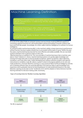
Types of Learning Styles for Machine Learning Algorithms
Wy ML Is important?

2
1. Machine learning applications can be found everywhere, throughout science, engineering, and
business, leading to more evidence-based decision-making.
2. Various automated AI recommendation systems are created using machine learning.
3. The enormous progress in machine learning has been driven by the development of novel
statistical learning algorithms along with the availability of big data (large data sets) and low-
cost computation.
What is the Deep Learning?
Deep Learning is a subset of Machine Learning.
It uses some ML techniques to solve real-world problems by tapping into neural networks that
simulate human decision-making.
Hence, Deep Learning trains the machine to do what the human brain does naturally.
What is semi-supervised learning?
Semi-supervised learning is a branch of machine learning that attempts to solve problems that require
or include both labelled and unlabelled data to train AI models. Semi-supervised learning employs
concepts of mathematics, such as characteristics of both clustering and classification methods.
Semi-supervised learning is an employable method due to the high availability of unlabelled samples
and the caveats of labelling large datasets with the utmost accuracy.
Furthermore, semi-supervised learning methods allow extending contextual information given by
labelled samples to a larger unlabelled dataset without significant accuracy loss.
Semi-supervised machine learning is useful in a variety of scenarios where labelled data is scarce or
expensive to obtain. For example, in medical imaging, manually annotating a large dataset can be
time-consuming and costly. In such cases, using a smaller set of labelled data in combination with a
larger set of unlabelled data can lead to improved model performance compared to using only
labelled data.

3
Supervised Learning / Predictive models:
Predictive model as the name suggests is used to predict the future outcome based on the historical
data. Predictive models are normally given clear instructions right from the beginning as in what needs
to be learnt and how it needs to be learnt. These class of learning algorithms are termed as Supervised
Learning.
For example: Supervised Learning is used when a marketing company is trying to find out which
customers are likely to churn. We can also use it to predict the likelihood of occurrence of perils like
earthquakes, tornadoes etc. with an aim to determine the Total Insurance Value. Some examples of
algorithms used are: Nearest neighbour, Naïve Bayes, Decision Trees, Regression etc.
Unsupervised learning / Descriptive models:
It is used to train descriptive models where no target is set and no single feature is important than the
other. The case of unsupervised learning can be: When a retailer wishes to find out what are the
combination of products, customers tends to buy more frequently. Furthermore, in pharmaceutical
industry, unsupervised learning may be used to predict which diseases are likely to occur along with
diabetes. Example of algorithm used here is: K- means Clustering Algorithm
Reinforcement learning (RL):
It is an example of machine learning where the machine is trained to take specific decisions based on
the business requirement with the sole motto to maximize efficiency (performance). The idea involved
in reinforcement learning is: The machine/ software agent trains itself on a continual basis based on
the environment it is exposed to, and applies it’s enriched knowledge to solve business problems. This

4
continual learning process ensures less involvement of human expertise which in turn saves a lot of
time!
An example of algorithm used in RL is Markov Decision Process.
Important Note: There is a subtle difference between Supervised Learning and Reinforcement
Learning (RL). RL essentially involves learning by interacting with an environment. An RL agent learns
from its past experience, rather from its continual trial and error learning process as against supervised
learning where an external supervisor provides examples.
A good example to understand the difference is self driving cars. Self driving cars use Reinforcement
learning to make decisions continuously – which route to take? what speed to drive on? are some of
the questions which are decided after interacting with the environment. A simple manifestation for
supervised learning would be to predict fare from a cab going from one place to another.
What are the applications of Machine Learning?
It is very interesting to know the applications of machine learning. Google and Facebook uses ML
extensively to push their respective ads to the relevant users. Here are a few applications that you
should know:
• Banking & Financial services: ML can be used to predict the customers who are likely to
default from paying loans or credit card bills. This is of paramount importance as machine
learning would help the banks to identify the customers who can be granted loans and credit
cards.
• Healthcare: It is used to diagnose deadly diseases (e.g. cancer) based on the symptoms of
patients and tallying them with the past data of similar kind of patients.
• Retail: It is used to identify products which sell more frequently (fast moving) and the slow
moving products which help the retailers to decide what kind of products to introduce or
remove from the shelf. Also, machine learning algorithms can be used to find which two /
three or more products sell together. This is done to design customer loyalty initiatives which
in turn helps the retailers to develop and maintain loyal customers.
These examples are just the tip of the iceberg. Machine learning has extensive applications practically
in every domain. You can check out a few Kaggle problems to get further flavor. The examples
included above are easy to understand and at least give a taste of the omnipotence of machine
learning.

6
Errors in Machine Learning?
if the machine learning model is not accurate, it can make predictions errors, and these prediction
errors are usually known as Bias and Variance. In machine learning, these errors will always be present
as there is always a slight difference between the model predictions and actual predictions. The main
aim of ML/data science analysts is to reduce these errors in order to get more accurate results.
Errors in Machine Learning?

7
In machine learning, an error is a measure of how accurately an algorithm can make predictions for
the previously unknown dataset. On the basis of these errors, the machine learning model is selected
that can perform best on the particular dataset. There are mainly two types of errors in machine
learning, which are:
o Reducible errors: These errors can be reduced to improve the model accuracy. Such errors
can further be classified into bias and Variance.
o Irreducible errors: These errors will always be present in the model
regardless of which algorithm has been used. The cause of these errors is unknown variables whose
value can't be reduced.
What is Bias?
In general, a machine learning model analyses the data, find patterns in it and make predictions. While
training, the model learns these patterns in the dataset and applies them to test data for
prediction. While making predictions, a difference occurs between prediction values made by the
model and actual values/expected values, and this difference is known as bias errors or Errors
due to bias. It can be defined as an inability of machine learning algorithms such as Linear Regression
to capture the true relationship between the data points. Each algorithm begins with some amount of
bias because bias occurs from assumptions in the model, which makes the target function simple to
learn. A model has either:
o Low Bias: A low bias model will make fewer assumptions about the form of the target
function.
o High Bias: A model with a high bias makes more assumptions, and the model becomes
unable to capture the important features of our dataset.
o A high bias model also cannot perform well on new data.
AD
Generally, a linear algorithm has a high bias, as it makes them learn fast. The simpler the algorithm,
the higher the bias it has likely to be introduced. Whereas a nonlinear algorithm often has low bias.
Some examples of machine learning algorithms with low bias are Decision Trees, k-Nearest
Neighbours and Support Vector Machines. At the same time, an algorithm with high bias is Linear
Regression, Linear Discriminant Analysis and Logistic Regression.

8
Ways to reduce High Bias:
High bias mainly occurs due to a much simple model. Below are some ways to reduce the high bias:
o Increase the input features as the model is underfitted.
o Decrease the regularization term.
o Use more complex models, such as including some polynomial features.
What is a Variance Error?
The variance would specify the amount of variation in the prediction if the different training data was
used. In simple words, variance tells that how much a random variable is different from its
expected value. Ideally, a model should not vary too much from one training dataset to another,
which means the algorithm should be good in understanding the hidden mapping between inputs
and output variables. Variance errors are either of low variance or high variance.
Low variance means there is a small variation in the prediction of the target function with changes in
the training data set. At the same time, High variance shows a large variation in the prediction of the
target function with changes in the training dataset.
A model that shows high variance learns a lot and perform well with the training dataset, and does not
generalize well with the unseen dataset. As a result, such a model gives good results with the training
dataset but shows high error rates on the test dataset.
Since, with high variance, the model learns too much from the dataset, it leads to overfitting of the
model. A model with high variance has the below problems:
o A high variance model leads to overfitting.
o Increase model complexities.
Usually, nonlinear algorithms have a lot of flexibility to fit the model, have high variance.
Some examples of machine learning algorithms with low variance are, Linear Regression, Logistic
Regression, and Linear discriminant analysis. At the same time, algorithms with high variance
are decision tree, Support Vector Machine, and K-nearest neighbours.
Ways to Reduce High Variance:
o Reduce the input features or number of parameters as a model is overfitted.
o Do not use a much complex model.
o Increase the training data.
o Increase the Regularization term.
Bias-Variance Trade-Off

9
While building the machine learning model, it is really important to take care of bias and variance in
order to avoid overfitting and underfitting in the model. If the model is very simple with fewer
parameters, it may have low variance and high bias. Whereas, if the model has a large number of
parameters, it will have high variance and low bias. So, it is required to make a balance between bias
and variance errors, and this balance between the bias error and variance error is known as the Bias-
Variance trade-off.
For an accurate prediction of the model, algorithms need a low variance and low bias. But this is not
possible because bias and variance are related to each other:
o If we decrease the variance, it will increase the bias.
o If we decrease the bias, it will increase the variance.
Bias-Variance trade-off is a central issue in supervised learning. Ideally, we need a model that
accurately captures the regularities in training data and simultaneously generalizes well with the
unseen dataset. Unfortunately, doing this is not possible simultaneously. Because a high variance
algorithm may perform well with training data, but it may lead to overfitting to noisy data. Whereas,
high bias algorithm generates a much simple model that may not even capture important regularities
in the data. So, we need to find a sweet spot between bias and variance to make an optimal model.
Hence, the Bias-Variance trade-off is about finding the sweet spot to make a balance between
bias and variance errors.
What is Bias?
The bias is known as the difference between the prediction of the values by the Machine
Learning model and the correct value. Being high in biasing gives a large error in training as well
as testing data. It recommended that an algorithm should always be low-biased to avoid the
problem of underfitting. By high bias, the data predicted is in a straight line format, thus not fitting
accurately in the data in the data set. Such fitting is known as the Underfitting of Data. This
happens when the hypothesis is too simple or linear in nature. Refer to the graph given below for
an example of such a situation.

10
High Bias in the Model
In such a problem, a hypothesis looks like follows.
What is Variance?
The variability of model prediction for a given data point which tells us the spread of our data is
called the variance of the model. The model with high variance has a very complex fit to the
training data and thus is not able to fit accurately on the data which it hasn’t seen before. As a
result, such models perform very well on training data but have high error rates on test data.
When a model is high on variance, it is then said to as Overfitting of Data. Overfitting is fitting the
training set accurately via complex curve and high order hypothesis but is not the solution as the
error with unseen data is high. While training a data model variance should be kept low. The high
variance data looks as follows.
High Variance in the Model
In such a problem, a hypothesis looks like follows.

11
Bias Variance Tradeoff
If the algorithm is too simple (hypothesis with linear equation) then it may be on high bias and low
variance condition and thus is error-prone. If algorithms fit too complex (hypothesis with high
degree equation) then it may be on high variance and low bias. In the latter condition, the new
entries will not perform well. Well, there is something between both of these conditions, known
as a Trade-off or Bias Variance Trade-off. This tradeoff in complexity is why there is a tradeoff
between bias and variance. An algorithm can’t be more complex and less complex at the same
time. For the graph, the perfect tradeoff will be like this.
We try to optimize the value of the total error for the model by using the Bias-Variance Tradeoff.
The best fit will be given by the hypothesis on the tradeoff point. The error to complexity graph to
show trade-off is given as –

12
Regarding general Scientific Theory, Occam's Razor states: Given two different explanations which
offer the same hypothesis, preference should be given to the simpler explanation. This is to reduce the
number of falsifiable assumptions for which your hypothesis relies, thereby keeping the hypothesis
robust.
Applied to Machine Learning this involves simplifying the algorithm on your training dataset to a less
complex model so that the testing sample is optimised for lowest prediction error. In fact one should
optimise the average of several testing datasets by way of a cross-validation applied to multiple train-
test splits.
This is because an overly complicated pattern may produce impressive results on the trained dataset
but does not generalise well; producing noise rather than the underlying predictive pattern. Data
Scientists call this "Overfitting" and can be a trap for a novice due to what may initially look like many
micro trends actually being just noise in the training data.
This is summarised as "the bias-variance trade-off" for the prediction error and is mathematically
expressed as:

13
Reducible error = Bias^2 + Var
Of course, the exact model chosen depends on the task you are undertaking, however for any given
model, the critical omnipresent principle is that increasing complexity will give a lower bias but higher
variance. For a robust algorithm which can be generalised these must be balanced.
Underfitting and Overfitting in Various Scenarios
Region for the Least Value of Total Error
This is referred to as the best point chosen for the training of the algorithm which gives low error
in training as well as testing data.
These Three Theories Help Us Understand Overfitting and Underfitting in Machine Learning Models
Occam’s Razor, VC Dimension, and the No-Free Lunch Theorem can help us think about overfitting
and underfitting in ML solutions.
Underfitting and overfitting are omnipresent challenges in modern machine learning(ML) solutions.
Both challenges are related to the capacity of a machine learning model to build relevant knowledge
based on an initial set of training examples. Conceptually, underfitting is associated with the inability of
a Machine Learning algorithm to infer valid knowledge from the initial training data. Contrary to that,
overfitting is associated with models that create hypotheses that are way too generic or abstract to
result in practical. Putting it in simpler terms, underfitting models are sort of dumb while overfitting
models tend to hallucinate(imagine things that don’t exist ) :).

14
One of the best ways to quantify the propensity to overfit or underfit in an ML model is to understand
its capabilities. Conceptually, Capacity represents the number of functions that a machine learning
model can select as a possible solution. for instance, a linear regression model can have all degree 1
polynomials of the form y = w*x + b as a Capacity (meaning all the potential solutions). Capacity is an
incredibly relevant concept in Machine Learning models. Technically, a machine learning algorithm
performs best when it has a capacity that is proportional to the complexity of its task and the input of
the training data set. Machine learning models with low Capacity are impractical when comes to
solving complex tasks and tend to…

19
“All models are wrong, but some are useful”
Neil Mason

20
CDAO | Value Hunter
18 articles Follow
November 12, 2014
Open Immersive Reader
So said the statistician George Box. Just to clarify what he meant, Box went on say:
“Remember that all models are wrong; the practical question is how wrong do they have to be, to not
be useful?”
The increased use of data mining and predictive analytical techniques within organisations means that
executives will be exposed more and more often to the results of these approaches. They will be
increasingly using them to make recommendations or to decide on courses of action. So, how you
know how wrong the model is and whether it can be useful or not?
All models are wrong...
This is a statement of fact really rather than a controversial opinion. After all the best model of a
house is the house itself. A scale model of the house is one representation of the real thing and will
give you a 3D perspective but possibly not some of the detail that you’re looking for. The set of
architect’s drawings will potentially have the detail you’re looking for but it may be difficult to visualize
what the finished house might look like. A painting of the house set in its landscape will give you a
different context. If you’re building a house you may end using all three approaches to made
decisions about how the build should go.
It’s the same with analytical models as well. They are all representations of the real thing, simplified to
a greater or lesser degree. All of them are ‘wrong’ to a greater or lesser extent. So how can you tell
how wrong they are?
Most models have measures of error of one type or another. For example, in simple linear regression,
which probably most people are familiar with, the Correlation Coefficient is one basic measure of the
goodness of the fit of the model. It broadly explains how much of the variation in the data can be
explained by the model. But it’s only one measure of how good the model is and modelers will be
balancing that measure with other measures to come up with the 'best' model. That’s the art in the
science of statistical modelling.
...but some are useful.
We can get some idea of how ‘wrong’ a model is from metrics and statistics, but how do we know if
it’s ‘useful’? Whereas ‘wrong’ in this case is essentially an analytical concept, the notion of ‘useful’ is
really a commercial or business concept.
A model is probably useful if it helps me make better decisions and to reduce risks. But the 'best'
models are not necessarily the most useful. Here’s a couple of examples.
Cluster analysis is one technique for creating customer segments. These segments may be required to
drive some type of targeted marketing activity. Cluster analysis is what is known as an unsupervised
learning technique which broadly means you give it some data, it does its own thing and then gives
an answer. You then have to figure out what the answer is actually telling you.
The technique will give the best model it can from an algorithmic point of view but it may not be that
useful. For example, the segments may not add to your existing body of knowledge or they may not

21
be actionable. It may be then that a slightly poorer model may be more useful because you can
translate the segmentation into a marketing program you can execute on.
Another example is in econometric modelling. This technique is often used for demand forecasting or
marketing mix analysis. It’s possible to build quite elaborate models that explain a great deal about
what drives sales from marketing factors, to competitive factors, to macro-economic factors.
However the elaborate model can be difficult to use when you want to look at different scenarios or
forecast the impact of a change because there’s so much data that needs to be inputted into it that it
becomes a time-consuming and laborious process. In this case a simpler model may actually be more
effective because it’s easier to deploy.
So, if you’re reviewing some outputs from a piece of modelling work that’s been done, it’s always
useful to keep George Box in mind and ask yourself (or the modeler) a couple of questions:
1. “How wrong is it?” i.e. is the model robust enough and fit for purpose?
2. “What can I do with it?” i.e. is it useful? Will it help me make better decisions?
Model Complexity & Overfitting in Machine Learning
May 29, 2022 by Ajitesh Kumar · Leave a comment
In machine learning, model complexity and overfitting are related in a manner that the model
overfitting is a problem that can occur when a model is too complex due to different reasons. This can
cause the model to fit the noise in the data rather than the underlying pattern. As a result, the model
will perform poorly when applied to new and unseen data. In this blog post, we will discuss what
model complexity is and how you can avoid overfitting in your machine learning models by handling
the model complexity. As data scientists, it is of utmost importance to understand the concepts related
to model complexity and how it impacts the model overfitting.
Table of Contents
• What is model complexity & why it’s important?
• What’s model overfitting & how it’s related to model complexity?
• How to avoid model complexity and overfitting?
What is model complexity & why it’s important?
Model complexity is a key consideration in machine learning. Simply put, it refers to the number of
predictor or independent variables or features that a model needs to take into account in order to
make accurate predictions. For example, a linear regression model with just one independent variable
is relatively simple, while the model with multiple variables or non-linear relationships is more
complex. A model with a high degree of complexity may be able to capture more variations in the data,
but it will also be more difficult to train and may be more prone to overfitting. On the other hand, a
model with a low degree of complexity may be easier to train but may not be able to capture all the
relevant information in the data. Finding the right balance between model complexity and predictive
power is crucial for successful machine learning. The picture below represents a complex model
(extreme right) vis-a-vis a simple model (extreme left). Note the aspect of a number of parameters vis-
a-vis model complexity.

22
Model complexity is a measure of how accurately a machine learning model can predict unseen data,
as well as how much data the model needs to see in order to make good predictions. Model complexity
is important because it determines how generalizable a model is – that is, how well the model can be
used to make predictions on new, unseen data. With simple models and abundant data, the
generalization error is expected to be similar to the training error. With more complex models and
fewer examples, the training error is expected to go down but the generalization gap grows which can
also be termed model overfitting.
The following are key factors that govern the model complexity and impact the model accuracy with
unseen data:
• The number of parameters: When there is a large number of tunable parameters,
which is also sometimes called the degrees of freedom, the models tend to be more
susceptible to overfitting.
• The range of values taken by the parameters: When the parameters can take a
wider range of values, models can become more susceptible to overfitting.
• The number of training examples: With a fewer or smaller number of datasets, it
becomes easier for models to overfit a dataset even if the model is simpler. Overfitting a
dataset with millions of training examples requires an extremely complex model.
Why is model complexity important? Because as models become more complex, they are more likely
to overfit the training data. This means that they may perform well on the training set but fail to
generalize to new data. In other words, the model has learned too much about the specific training set
and has not been able to learn the underlying patterns. As a result, it is essential to strike the right
balance between model complexity and overfitting when developing machine learning models.
What’s model overfitting & how it’s related to model complexity?
Model overfitting occurs when a machine learning model is too complex, captures noise in the training
data instead of the underlying signal, and therefore does not generalize well to new data. This is
usually due to the model having been trained on too small of a dataset, or on a dataset that is too
similar to the test dataset. The picture below represents the relationship between model complexity
and training/test (generalization) prediction error.

23
Note some of the following in the above picture:
• As the model complexity increases (x-direction), the training error decreases, and the
test error increases.
• When the model is very complex, the gap between training and generalization/test error
is very high. This is the state of overfitting
• When the model is very simple (less complex), the model will have a sufficiently high
training error. The model is said to be underfitting.
In the case of the neural networks, model complexity can be increased by adding more hidden layers
to the model, or by increasing the number of neurons in each layer. Model overfitting can be
prevented by using regularization techniques such as dropout or weight decay. When using these
techniques, it is important to carefully choose the appropriate level of regularization, as too much
regularization can lead to underfitting.
How to avoid model complexity and overfitting?
In machine learning, one of the main goals is to find a model that accurately predicts the output for
new input data. However, it is also important to avoid both model complexity and overfitting. When
models are too complex, they tend to overfit the training data and perform poorly on new, unseen
data. This is because they have learned the noise in the training data rather than the underlying signal.
Model complexity can also lead to longer training times and decreased accuracy, while overfitting can
cause the model to perform well on the training data but poorly on new data. There are a few ways to
prevent these problems.
• Use simpler models: This may seem counterintuitive, but simpler models are often
more robust and generalize better to new data. One way to create simpler models is by
avoiding too many features. If a model has too many features, it may start to overfit the
data. It is important to select only the most relevant features for the model.
• Use regularization techniques, which help to avoid creating overly complex models
by penalizing excessive parameter values. It adds a penalty to the loss function that is
proportional to the size of the weights. Common regularization techniques include L1
(Lasso) and L2 (Ridge) regularization. For example, Lasso regression is a type of linear
regression that uses regularization to reduce model complexity and prevent overfitting.
• Split the data into a training set and a test set, which allows the model to be
trained on one set of data and then tested on another. This can help prevent overfitting
by ensuring that the model generalizes well to new data.
• Use early stopping: Early stopping is another technique that can be used to prevent
overfitting. It involves training the model until the validation error starts to increase and
then stopping the training process. This ensures that the model does not continue to fit
the training data after it has started to overfit.
• Use cross-validation: Cross-validation is a technique that can be used to reduce
overfitting by splitting the data into multiple sets and training on each set in turn. This
allows the model to be trained on different data and prevents it from being overfitted to a
particular set of data.
• Monitor the performance of the model as it is trained and adjust the parameters
accordingly.
Model complexity and overfitting are two of the main problems that can occur in machine learning.
Model complexity can lead to a model that is too complex and does not generalize well to new data,
while overfitting can cause the model to perform well on the training data but poorly on new data.
There are several ways to prevent these problems, including using simpler models, using
regularization techniques, splitting the data into a training set and a test set, early stopping, and cross-
validation. It is important to monitor the performance of the model as it is being trained and adjust
the parameters accordingly.
1.2. Mathematical Modeling
Any branch of science, as it progresses from qualitative to quantitative, is likely to reach the
point where the use of mathematics to connect experiment and theory is essential.
Mathematical modeling consists of the following steps [44]:
1. Definitions;
2. Systems analysis;
3. Modeling;
4. Simulation;
5. Validation.

24
Mathematical models can be classified into mechanistic (white box), empirical (black box), and
hybrid (gray box). These, in turn, have sub-classifications, as shown in Figure 1 [36].
Figure 1. Classification of mathematical models. The diagram shows the three main classifications of
the white box, black box and gray box models, and their sub-classifications of the white box or
mechanistic, and black box or empirical models. Mechanistic and empirical models can be
deterministic or stochastic; and in turn, they can be continuous or discrete.
Empirical models, also called black box models, mainly described a system’s responses by
using mathematical or statistical equations without any scientific content, restrictions, or scientific
principle. Depending on particular goals, this may be the best type of model to build [44]. Its
construction is based only on experimental data and does not explain dynamic mechanisms; this
refers to the fact that the system’s process is unknown [40]. Estimating an unknown function from the
observations of its values is a problem. The basic advice in this aspect is to estimate models of
different complexity and evaluate them using validation data. A good way to restrict certain classes of
models’ flexibility is to use a regularized fit criterion. A key issue is finding a sufficiently flexible
parameterization model. Another key is to find a suitable “close approach “to the model structure [45].
Researchers usually employ methods for predicting physiological parameters by using intelligent
algorithms, such as Support Vector Machines (SVM), Back-Propagation Neural Network (BPNN),
Artificial Neural Network (ANN), Deep Neural Network (DNN), and the combination of Wide and Deep
Neural Network (WDNN) [46].
Mechanistic models, also called white box models, provide a degree of understanding or
explanation of the modeled phenomena. The term “understanding” implies a causal relationship
between quantities and mechanisms (processes). A well-built mechanistic model is transparent and
open to modifications and extensions, more or less without limits. A mechanistic model is based on
our ideas about how the system works, the important elements, and how they are related [44]. These
models allow knowing the input or output variables and the variables involved during the modeling
process [40,47]. Mechanistic models are more research-oriented than application-oriented, although
this is changing as our mechanistic models become more reliable. Evaluation of such models is
essential, although it is often, and inevitably, rather subjective. Conventional mechanistic models are
complex, and unfriendly [44].
Figure 1 shows that both mechanistic and empirical models can be deterministic or stochastic.
Determinists make definite quantitative predictions (plant dry-matter or animal intake) without any
associated probability distribution. This can be acceptable in many cases; however, it may not be
satisfactory for quite changeful quantities or processes (e.g., rain or the migration of diseases, pests,
or predators). On the other hand, stochastic models include a random element as a part of the model
so that the predictions have a distribution. One problem with stochastic models is that they can be
technically difficult to build and complex to test or falsify [44].
In turn, the deterministic and stochastic models can be continuous or discrete. A mathematical
model that describes the relationship between continuous signals in time is called time-continuous.
Differential equations are frequently used to describe such relationships. A model that directly relates

25
the values of the signals at the sampling times is called a discrete or sampled time model. Such a
model is typically described by differential equations [48].
The continuous models are classified as dynamic since they predict how quantities vary with
time, so a dynamic model is generally presented as a set of ordinary differential equations with time
(t), the independent variable. On the other hand, the continuous models can also be static; they do
not contain time as a variable and do not make time-dependent predictions [44].
Finally, dynamic models can be grouped or distributed. Partial differential equations
mathematically describe many physical phenomena. The events in the system are, so to speak,
scattered over the spatial variables. This description is called the distributed parameter model. If a
finite number of changing variables describes the events, we speak of grouped models. These models
are usually expressed by ordinary differential equations [48].
An intermediate model is classified as the semi-empirical or semi-mechanistic model between
the black box and white box models. These models are also called gray box or hybrid models; they
consist of a combination of empirical and mechanistic models [40].
The practical use of a mathematical model classification lies in understanding “where you are” in
the mathematical model space and what types of models might apply to the problem. To understand
the nature of mathematical models, they can be defined by the chronological order in which the
model’s constituents usually appear. Usually, a system is given first, then there is a question regarding
that system, and only then is a mathematical model developed. This process is denoted as SQM,
where S is a system, Q is a question relative to S, and M is a set of mathematical states M = (σ1, σ2,
…, Σn) which can be used to answer Q. Based on this definition, it is natural to classify mathematical
models in an SQM space [36]. Figure 2 shows an approach to visualize this SQM space of
mathematical models based on the white box and black box models classification. At the black box, at
the beginning of the spectrum, models can perform reliable predictions based on data. At the white
box end of the spectrum, mathematical models can be applied to the design, testing, and optimization
of computer processes before they are physically carried out. On each of the S, Q, and M axes
in Figure 2b, the mathematical models are classified based on a series of criteria compiled from
various classification attempts in the literature [36].
Figure 2. The three dimensions of an SQM mathematical model, where the (S) systems are ranked at
the top of the bar; immediately below the bar, there is a list of objectives that the mathematical models
in each of the segments can have (which is Q); at the lower end are the corresponding mathematical
structures (M) ranging from algebraic equations (Aes) to differential equations (Des). (a) Classification
of mathematical models between black and white box models. (b) Classification of mathematical
models in the SQM space. Modified from [36].

26
There are different mathematical models related to biochemical, physical, and agroecological
variables that estimate photosynthesis at the leaf, plant, or group of plant levels. Therefore, the study
of mathematical modeling focused on the photosynthetic process becomes important in the
agricultural sector. Since it is a direct indicator of a plant’s health. It also makes it possible to assess
the consequences of global climate change on crop growth, since the high concentration of CO2, the
increase in temperature and altered rainfall patterns can have serious effects on crop production in
the near future [44].
However, to the best of the authors’ knowledge, a study on the diversity of mathematical
modeling in the field of scientific research has not been approached nor focused on: the mathematical
formulation, the complexity of the model, the validation, the type of crop (at the leaf, plant or canopy
level), the analysis of the diversity of variables used with their respective units, as well as the
invasiveness in their measurements. Hence, this manuscript presents a selective review of
mathematical modeling to estimate photosynthesis.
In the literature, there is a review of the mathematical modeling of photosynthesis developed by
Susanne Von Caemmerer. However, here only several models derived from the C3 model by
Farquhar, von Caemmerer, and Berry are discussed and compared. The models described and
reviewed here describe the assimilation rates of CO2 in a steady state and provide a set of
hypotheses collected in a quantitative way that can be used as research tools to interpret experiments
both in the field and in the laboratory. Additionally, it also provides tools for reflective experiments [49].
Conversely, the present paper provides a new vision of the state of the art in mathematical models
with certain specifications. This information can be used to develop new mathematical models to
estimate photosynthesis with new variables related to the plant’s habitat and with greater relevance to
be implemented in electronic systems during the development of photosynthesis estimation
equipment.
Politics
Election Update: The Case For And Against Democratic Panic
Election Update: The Case For And Against Democratic Panic
By Nate Silver
Filed under 2016 Election
BETHANY HECK
Want these election updates emailed to you right when they’re published? Sign up here.
Last Friday, I wrote an article titled “Democrats Should Panic … If The Polls Still Look Like This In A
Week.” Well, it’s been a week — actually eight days — since that was published. So: Should Democrats
panic?
The verdict is … I don’t know. As of a few days ago, the case for panic looked pretty good. But Hillary
Clinton has since had some stronger polls and improved her position in our forecast. In our polls-only
model, Clinton’s chances of winning are 61 percent, up from a low of 56 percent earlier this week, but
below the 70 percent chance she had on Sept. 9, before her “bad weekend.”
The polls-plus forecast has followed a similar trajectory. Clinton’s chances of winning are now 60
percent, up from a low of 55 percent but worse than the 68 percent chance she had two weeks ago.

27
I’d love to give the polls another week to see how these dynamics play out. Even with a fairly
aggressive model like FiveThirtyEight’s, there’s a lag between when news occurs and when its impact
is fully reflected in the polls and the forecast. But instead, Monday’s presidential debate is likely to
sway the polls in one direction or another — and will probably have a larger impact on the race than
whatever shifts we’ve seen this week.
There’s also not much consensus among pollsters about where the race stands. On the one hand, you
can cite several national polls this week that show Clinton ahead by 5 or 6 percentage points, the first
time we’ve consistently seen numbers like that in a few weeks. She also got mostly favorable numbers
in “must-win states,” such as New Hampshire. But Clinton also got some pretty awful polls this
week in other swing states: surveys from high-quality pollsters showing her 7 points behind Donald
Trump in Iowa, or 5 points behind him in Ohio, only tied with him in Maine, for instance. The
differences are hard to reconcile: It’s almost inconceivable that Clinton is both winning nationally by 6
points and losing Ohio (for example) by 5 points.
I usually tell people not to sweat disagreements like these all that much. In fact, most observers
probably underestimate the degree of disagreement that occurs naturally and unavoidably between
polls because of sampling error, along with legitimate methodological differences over techniques
such as demographic weighting and likely-voter modeling.1 If anything, there’s usually
too little disagreement between pollsters because of herding, which is the tendency to suppress
seeming “outlier” results that don’t match the consensus.
Still, the disagreement between polls this week was on the high end, and that makes it harder to know
exactly what the baseline is heading into Monday’s debate. The polls-only model suggests that Clinton
is now ahead by 2 to 3 percentage points, up slightly from a 1- or 2-point lead last week. But I wouldn’t
spend a lot of time arguing with people who claim her lead is slightly larger or smaller than that. It
may also be that both Clinton and Trump are gaining ground thanks to undecided and third-party
voters, a trend that could accelerate after the debate because Gary Johnson and Jill Stein won’t appear
on stage.
In football terms, we’re probably still in the equivalent of a one-score game. If the next break goes in
Trump’s direction, he could tie or pull ahead of Clinton. A reasonable benchmark for how much the
debates might move the polls is 3 or 4 percentage points. If that shift works in Clinton’s favor, she
could re-establish a lead of 6 or 7 percentage points, close to her early-summer and post-convention
peaks. If the debates cut in Trump’s direction instead, he could easily emerge with the lead. I’m not
sure where that ought to put Democrats on the spectrum between mild unease and full-blown panic.
The point is really just that the degree of uncertainty remains high.
WBUR
LOCAL COVERAGE
LISTEN LIVE: On Point
DONATE
Home//Local Coverage

28
Is 'Google Flu Trends' Prescient Or Wrong?
Google
in blue, CDC in red. Note the dramatic divergence toward 2013. (Keith Winstein, MIT)
Has Google’s much-celebrated flu estimator, Google Flu Trends, gotten a bit, shall we say, over-enthusiastic?
Last week, a friend commented to Keith Winstein, an MIT computer science graduate student and former
health care reporter at The Wall Street Journal: “Whoa. This flu season seems to be the worst ever. Check out
Google Flu Trends.”
WBUR is a nonprofit news organization. Our coverage relies on your financial support. If you value
articles like the one you're reading right now, give today.
Hmmm, Winstein responded. When he checked, he saw that the official CDC numbers showed the flu getting
worse, but not nearly at Google’s level. (See the graph above.) The dramatic divergence between the Google
data and the official CDC numbers struck him: Was Google, he wondered, prescient or wrong?
He began to explore — as much as a heavy grad-student schedule allows — and shares his thoughts here. Our
conversation, lightly edited:
I accept the caveat that these predictive algorithms are not your speciality, but still, from highly informed,
casual observation, what are you seeing, in a highly preliminary sort of way?
Well, I'm certainly not an expert on the flu. The issue that’s interesting from the computer science perspective
is this: Google Flu Trends launched to much fanfare in 2008 — it was even on the front page of the New York
Times — with this idea that, as the head of Google.org said at the time, they could out-perform the CDC’s very
expensive surveillance system, just by looking at the words that people were Googling for and running them
through some statistical tools.
It’s a provocative claim and if true, it bodes well for being able to track all kinds of things that might be relevant
to public health. Google has since launched Flu Trends sites for countries around the world, and a dengue fever
site.
So this is an interesting idea, that you could do public health surveillance and out-perform the public health
authorities [which use lab tests and reports from ‘sentinel’ medical sites] just by looking at what people were
searching for.
'It is often a problem with computers that they only tell us things we already know.'
Google was very clear that it wouldn’t replace the CDC, but they have said they would out-perform the CDC.
And because they’re about 10 days earlier than the CDC, they might be able to save lives by directing anti-viral
drugs and vaccines to afflicted regions.
And their initial paper in the journal Nature said the Google Flu Trends predictions were 97% accurate...

29
That was astounding. However, it is often a problem with computers that they only tell us things we already
know. When you give a computer something unexpected, it does not handle it as well as a person would.
Shortly after that report of 97% accuracy, we had that unexpected swine flu, which was a different time of year
from the normal flu season, and it was different symptoms from normal, and so Google’s site didn’t work very
well.
And the accuracy went down to 20-something percent?
To a 29 percent correlation, and it had just been 97 percent. So it was not accurate. And what Google is
predicting is not the most important measure of flu intensity. What they predict is the easiest measure, which
is the percentage of people who go to the doctor and have an “influenza-like illness.” You can imagine that’s
related to people who search for things like fever on the Internet. But generally what public health agencies
consider more important are measurements on lab tests to determine who actually has the flu.
Google had tried and so far has not been successful at predicting the real flu. This is another illustration of how
computers can tell us things that are not always what we want to know.
In 2009, Google retooled their algorithm, and did what they called their first annual update to correct the
under-estimate they had during swine flu. They brought the accuracy back up again, based on new evidence
about what people searched for during swine flu. And that was the last annual update, in the fall of 2009. They
say further annual updates have not been necessary.
And now we are in early 2013, and they’re predicting super-high levels. The CDC reported Friday [Jan. 11] that
for the week of December 30, 2012, through January 5, 2013, 4.3% of doctor visits were by patients with
influenza like illness, down from 5.6% the previous week. By contrast, on Jan. 6 Google finalized its prediction
for the same statistic at 8.6%, up from 7.9% the previous week. This difference is larger than has ever occurred
before. The current Google estimate (for the week of 1/6) is 9.6%, with no sign of a decline yet.
So what do you think is going on, that they’re so different?
It is too soon to tell whether Google is wrong or just prescient. because both Google and the CDC’s numbers
have been going up rapidly. It’s true that Google has been high, but maybe they’re just early. If next week the
CDC says, ‘Hey, flu just went up to 9 percent,” we’ll say Google was great, they were early, they gave good
warnings.
'This could be a cautionary tale about the perils of relying on these "Big Data" predictive models in
situations where accuracy is important.'
One person at Google said in an email that because this is such an early flu season, they suspect people’s
behavior going to the doctor around the week of Christmas might be different. They think the worried well,
people who are ultimately not sick but just worried about it, are going to be less likely to go to the doctor over
Christmas, so though they might search for symptoms they won’t go to the doctor, and that might explain why
the search numbers are high but the actual doctor numbers are lower.
But the actual virological numbers are even lower, and Google has never trained the algorithm on a Christmas
flu season. So its not something the computer would necessarily know to expect.
Another possibility is, just as the 2008 algorithm under-estimated the 2009 flu, the retooled 2009 algorithm is
overestimating the 2012-2013 flu. It will be hard to render a definitive judgment until we have the benefit of
hindsight. But depending on how it shakes out, this could be a cautionary tale about the perils of relying on
these "Big Data" predictive models in situations where accuracy is important.
We plan a follow-up as we get more information, and we asked Google for comment. In an email, Kelly Mason
of Google.org's Global Communications and Public Affairs team, responded:
I think the most important point is that data is still coming in, with some regions reporting flu activity more
quickly than others. (The disclaimer the CDC uses is below). Basically - it's still early.
In past years, CDC reports are updated as new information comes in. We validate the FluTrends model each
year. Since a 2009 update, we've seen the model perform well each flu season with no additional updates
required. If you have more specific questions, please do let me know.
From the CDC:
"As a result of the end of year holidays and elevated influenza activity, some sites may be experiencing longer
than normal reporting delays and data in previous weeks are likely to change as additional reports are
received."
http://www.cdc.gov/flu/weekly/
Readers, thoughts? Anybody placing any bets on whose estimates will prove most accurate?
(Updated at 3:06 p.m. with Google comment. Updated 6:20, changing Google flu "predictor" to "estimator." )
This program aired on January 13, 2013. The audio for this program is not available
Baseline models for machine learning
By Christina Ellis / August 23, 2021 / Machine learning, Soft skills / 1 Comment

30
Share this article
Are you wondering why you should use baseline models for machine learning? Or maybe you are
more interested in hearing more about how to build baseline models for machine learning? Either
way, we’ve got you covered! In this article we tell you everything you need to know about building
baseline models for machine learning.
In the beginning of this article, we discuss what a baseline model for a machine learning project is.
After that, we talk about why you should build a baseline model for each of your machine learning
projects. Finally, we provide examples of different kinds of baseline models you can use in your
machine learning projects.
What is a baseline model?
What is a baseline model in a machine learning project? A baseline model is a very simple model that
you can create in a short amount of time. Your baseline model should be created using the same data
and outcome variable that will be used to create your actual model. Baseline modes can be simple
stochastic models or they can be built on rule-based logic.
Generally speaking, if your actual model is a complex, highly parameterized model then a simple
stochastic model would be an appropriate baseline. If your actual model is a fairly simple stochastic
model, then a simple baseline that uses easy to implement business logic may be more appropriate.
Why use a baseline model for machine learning
Why should you use a baseline model for your machine learning projects? In the following section we
will go over some of the main reasons that you should use a baseline model in your machine learning
projects.
Understand your data faster
The first high level reason that you should use a baseline model in your machine learning projects is
because it helps you understand your data faster. Here are a few examples of how baseline models
help you to understand your data.
• Identify difficult to classify observations. By looking at the results of a baseline
model, you can get a sneak peak at which observations are the most difficult to
classify. You might see, for example, that one subset of your data was easy to classify
using simple business logic, but another subset was not so easily classified. This kind
of information can help inform the data you use in your model as well as your choice
of model.

31
• Identify different classes to classify. Similarly, if you are working on a multi-class
regression problem, using a baseline model can give you a preview of which classes
are easy to classify and which classes are difficult to classify. You might see, for
example, that two classes are very hard to distinguish from each other and decide to
group those classes together moving forward.
• Identify low signal data. If you create a baseline model and find that your model has
little to no prediction power, that might be an indicator that there is little signal in
your data. It is much better to find this out early on after building just a simple model
than later on after you have spent weeks building a highly complex model.
Compare your actual model to a benchmark
The next reason you should consider using a baseline mode for your machine learning projects is
because baseline models give a good benchmark to compare your actual models against.
• Utilize relative performance metrics. Some performance metrics such as log loss
are easier to use to compare one model to another than to evaluate on their own. This
is because many performance metrics do not have a defined scale and rather take on
different values depending on the range of the outcome variable. If you have a simple
baseline model, you now have a built in benchmark to measure your actual model
against. This can help you distinguish cases where a complex model is needed for
cases where simple business logic is sufficient.
• Estimate the potential impact on business metrics. Building out a simple baseline
model can also give you an idea of what kind of impact you might be able to have on
business metrics. This is especially true if your baseline model is also a stochastic
model.
Iterate with speed
Building baseline models also increases the speed with which you are able to develop models and
their downstream processes.
• Iterate on your model more quickly. Once you have a simple baseline model build
out, you have a good benchmark that you can build off of. This makes it easier to
determine whether the modifications you are making to your model actually improve
metrics or not, which allows you to identify and cease efforts that are not providing
value faster. This allows you to identify efforts that will improve your metrics faster.
• Unblock downstream processes. If you have a simple baseline model built out, this
also unblocks people who are working on downstream processes that depend on
your model and allows them to get to their work faster. For example, if an engineer is
helping you with your model deployment, they might be able to start their work using
your baseline model as a template while you iterate on the actual model.
• Progress to other projects faster. Building simple baseline models can also help you
complete your current project and move on to other projects faster. Why is that?
Because sometimes you will build a baseline model then realize that the baseline
model is sufficient for your use case. If you find that a quick simple model can get you
to the point you need to be at, there is no point in spending weeks or months
developing a more complex model.
How to create a baseline model
How do you create a baseline model? In this section, we will give you some examples of common
baseline models that are used in machine learning. Most of these models apply to structured tabular
data, but the concept of building a baseline model can certainly be extended to problems involving
unstructured data.
Baseline regression models
First we will discuss a few simple examples of baselines that can be used for regression problems. You
will notice that many of these examples do not involve any stochastic modeling at all.

32
• Mean or median. The first example of a baseline model we will provide is simply the
mean or median of your outcome variable. This just means that you would predict the
median value of the outcome variable for every single observation in the dataset. This
is an extremely simple benchmark that you can use as a baseline if your actual model
is a set of rules or business logic.
• Conditional mean or business logic. The next example is still a simple, deterministic
model. Simply choose a variable or two that you believe to be most strongly
associated with the outcome and build out some business logic that conditions on
those variables. For example, if you are trying to predict the height of a child,
you might condition on their age group and weight class that child falls into. You
might, for example, see that the median height for a child in the 5 – 8 year old age
group and 50 – 60 pound weight class is 4′ 2″ and decide to use that value for all
observations in that age group and weight class. This is a great avenue to pursue if
your main model is a relatively simple stochastic model like a linear regression.
• Linear regression. Finally, if you are using a complex model with a lot of features as
your main model then a simple linear regression model with a few features is a great
baseline model.
Baseline classification models
Now we will discuss baseline models that you can use for classification problems. If you pay close
attention, you will see that the models we suggest for classification problems are very similar to the
models we suggest for regression problems.
• Mode. For binary classification problems, the simplest baseline model you could think
of is just predicting the mode (or the most common class) of the outcome variable for
all observations. This is the analog to predicting the mean or median in regression
and is a great baseline model to use if your main model is a set of deterministic rules
or business logic.
• Conditional mode or business logic. If your actual model is a simple stochastic
model such as a logistic regression model, then it might be more appropriate to use a
conditional mode or simple business logic as your baseline model. For example, if you
are predicting whether a dog will eat more or less than 2 cups of food per day then
you might want to condition on the size of the dog. If, for example, you see that most
large dogs eat more than 2 cups of food then you should just classify all large dogs as
eating more than 2 cups.
• Logistic regression. Finally, if your actual classification model is a complex model
with a lot of features, then a simple stochastic model such as a logistic regression
model serves as a great baseline
How do I know this model will succeed? How will it perform in production?
To answer this important question, we need to understand how to evaluate a machine learning model.
This is one of the core tasks in a machine learning workflow, and predicting and planning for a model’s
success in production can be a daunting task.
What is Model Evaluation?
Model Evaluation is the process through which we quantify the quality of a system’s predictions. To do
this, we measure the newly trained model performance on a new and independent dataset. This model
will compare labeled data with it’s own predictions.
Model evaluation performance metrics teach us:
• How well our model is performing
• Is our model accurate enough to put into production
• Will a larger training set improve my model’s performance?
• Is my model under-fitting or over-fitting?
There are four different outcomes that can occur when your model performs classification predictions:
• True positives occur when your system predicts that an observation belongs to a class
and it actually does belong to that class.

33
• True negatives occur when your system predicts that an observation does not belong to
a class and it does not belong to that class.
• False positives occur when you predict an observation belongs to a class when in reality
it does not. Also known as a type 2 error.
• False negatives occur when you predict an observation does not belong to a class when
in fact it does. Also known as a type 1 error.
From the outcomes listed above, we can evaluate a model using various performance metrics.
Metrics for classification models
The following metrics are reported when evaluating classification models:
• Accuracy measures the proportion of true results to total cases. Aim for a high accuracy
rate.
accuracy = # correct predictions / # total data points
• Log loss is a single score that represents the advantage of the classifier over a random
prediction. The log loss measures the uncertainty of your model by comparing the
probabilities of it’s outputs to the known values (ground truth).. You want to minimize log
loss for the model as a whole.
• Precision is the proportion of true results over all positive results.
• Recall is the fraction of all correct results returned by the model.
• F1-score is the weighted average of precision and recall between 0 and 1, where the ideal
F-score value is 1.
• AUC measures the area under the curve plotted with true positives on the y axis and false
positives on the x axis. This metric is useful because it provides a single number that lets
you compare models of different types.
Confusion Matrix the correlation between the label and the model’s classification. One axis of a confusion
matrix is the label that the model predicted, and the other axis is the
ROC Chart
The ROC chart is similar to the gain or lift charts in that they provide a means of comparison between classification
models. The ROC chart shows false positive rate (1-specificity) on X-axis, the probability of target=1 when its true
value is 0, against true positive rate (sensitivity) on Y-axis, the probability of target=1 when its true value is
1. Ideally, the curve will climb quickly toward the top-left meaning the model correctly predicted the cases. The
diagonal red line is for a random model (ROC101).
Area Under the Curve (AUC)
Area under ROC curve is often used as a measure of quality of the classification models.
A random classifier has an area under the curve of 0.5, while AUC for a perfect classifier is equal to 1.
In practice, most of the classification models have an AUC between 0.5 and 1.

34
An area under the ROC curve of 0.8, for example, means that a randomly selected case from the group with the
target equals 1 has a score larger than that for a randomly chosen case from the group with the target equals 0 in
80% of the time. When a classifier cannot distinguish between the two groups, the area will be equal to 0.5 (the ROC
curve will coincide with the diagonal). When there is a perfect separation of the two groups, i.e., no overlapping of
the distributions, the area under the ROC curve reaches to 1 (the ROC curve will reach the upper left corner of the
plot
F1 Score [Image 9] (Image courtesy: My Photoshopped Collection)
It is difficult to compare two models with low precision and high recall or vice versa. So to make them
comparable, we use F-Score. F-score helps to measure Recall and Precision at the same time. It uses
Harmonic Mean in place of Arithmetic Mean by punishing the extreme values more.
How To Estimate FP, FN, TP, TN, TPR, TNR, FPR, FNR & Accuracy for Multi-Class Data in Python in 5
minutes
In this post, I explain how someone can read a confusion matrix and how to extract several
performance metrics for a multi-class classification problem from the confusion matrix in 5 minutes
1. Introduction
In one of my previous posts, “ROC Curve explained using a COVID-19 hypothetical example: Binary &
Multi-Class Classification tutorial”, I clearly explained what a ROC curve is and how it is connected
to the famous Confusion Matrix. If you are not familiar with the term Confusion Matrix and True
Positives, True Negatives, etc., refer to the above article and learn everything in 5
minutes or continue reading for a quick 2 minutes recap.

35
2. A quick recap: what do TP
, TN, FP, and FN mean?
Let’s imagine that we have a test that is able within seconds to tell us if one individual is affected by
the virus or not. So the output of the test can be either Positive (affected) or Negative (not
affected). So, in this hypothetical case, we have a binary classification case.
Handmade sketch made by the author. An example of 2 populations, one affected by covid-19 and the other
not affected, assuming that we really know the ground truth. Additionally, based on the output of the test, we
can denote a person as affected (blue population) or not affected (red population).
• True Positives (TP, blue distribution) are the people that truly have the virus.
• True Negatives (TN, red distribution) are the people that truly DO NOT have the
virus.
• False Positives (FP) are the people that are truly NOT sick, but based on the test,
they were falsely (False) denoted as sick (Positives).
• False Negatives (FN) are the people that are truly sick, but based on the test, they
were falsely (False) denoted as NOT sick (Negative).
To store all these measures of performance, the confusion matrix is usually used.
If you want to learn Data Science by yourself with the support of interactive roadmaps and an active
learning community have a look at this resource: https://aigents.co/learn
3. The Confusion Matrix: Getting the TPR, TNR, FPR, FNR.

36
Classification: ROC Curve and
AUC

38
What is a confusion matrix?·
Everything you Should Know about Confusion Matrix for Machine Learning

39
A Confusion matrix is an N x N matrix used for evaluating the performance of a classification
model, where N is the number of target classes. The matrix compares the actual target values with
those predicted by the machine learning model.
Binary Classification Problem (2x2 matrix)
1. A good model is one which has high TP and TN rates, while low FP and FN rates.
2. If you have an imbalanced dataset to work with, it’s always better to use confusion
matrix as your evaluation criteria for your machine learning model.
A confusion matrix is a tabular summary of the number of correct and incorrect
predictions made by a classifier. It is used to measure the performance of a classification model. It
can be used to evaluate the performance of a classification model through the calculation of
performance metrics like accuracy, precision, recall, and F1-score.

40
Confusion matrices are widely used because they give a better idea of a model’s performance than
classification accuracy does. For example, in classification accuracy, there is no information about the
number of misclassified instances. Imagine that your data has two classes where 85% of the data
belongs to class A, and 15% belongs to class B. Also, assume that your classification model
correctly classifies all the instances of class A, and misclassifies all the instances of class B. In this case,
the model is 85% accurate. However, class B is misclassified, which is undesirable. The confusion
matrix, on the other hand, displays the correctly and incorrectly classified instances for all the classes
and will, therefore, give a better insight into the performance of your classifier.
We can measure model accuracy by two methods. Accuracy simply means the number of values
correctly predicted.
1. Confusion Matrix
2. Classification Measure
1. Confusion Matrix
a. Understanding Confusion Matrix:
The following 4 are the basic terminology which will help us in determining the metrics we are looking
for.
• True Positives (TP): when the actual value is Positive and predicted is also Positive.
• True negatives (TN): when the actual value is Negative and prediction is also Negative.
• False positives (FP): When the actual is negative but prediction is Positive. Also known
as the Type 1 error
• False negatives (FN): When the actual is Positive but the prediction is Negative. Also
known as the Type 2 error
For a binary classification problem, we would have a 2 x 2 matrix as shown below with 4 values:

41
Confusion Matrix for the Binary Classification
• The target variable has two values: Positive or Negative
• The columns represent the actual values of the target variable
• The rows represent the predicted values of the target variable
b. Understanding Confusion Matrix in an easier way:
Let’s take an example:
We have a total of 20 cats and dogs and our model predicts whether it is a cat or not.
True Positive (TP) = 6
You predicted positive and it’s true. You predicted that an animal is a cat and it actually is.
True Negative (TN) = 11

42
You predicted negative and it’s true. You predicted that animal is not a cat and it actually is not (it’s a
dog).
False Positive (Type 1 Error) (FP) = 2
You predicted positive and it’s false. You predicted that animal is a cat but it actually is not (it’s a dog).
False Negative (Type 2 Error) (FN) = 1
You predicted negative and it’s false. You predicted that animal is not a cat but it actually is.
2. Classification Measure
Basically, it is an extended version of the confusion matrix. There are measures other than the
confusion matrix which can help achieve better understanding and analysis of our model and its
performance.
a. Accuracy
b. Precision
c. Recall (TPR, Sensitivity)
d. F1-Score
e. FPR (Type I Error)
f. FNR (Type II Error)
a. Accuracy:
Accuracy simply measures how often the classifier makes the correct prediction. It’s the ratio between
the number of correct predictions and the total number of predictions.
The accuracy metric is not suited for imbalanced classes. Accuracy has its own disadvantages,
for imbalanced data, when the model predicts that each point belongs to the majority class label, the
accuracy will be high. But, the model is not accurate.
It is a measure of correctness that is achieved in true prediction. In simple words, it tells us how
many predictions are actually positive out of all the total positive predicted.
Accuracy is a valid choice of evaluation for classification problems which are well
balanced and not skewed or there is no class imbalance.

43
b. Precision:
It is a measure of correctness that is achieved in true prediction. In simple words, it tells us how
many predictions are actually positive out of all the total positive predicted.
Precision is defined as the ratio of the total number of correctly classified positive classes divided by
the total number of predicted positive classes. Or, out of all the predictive positive classes, how much
we predicted correctly. Precision should be high(ideally 1).
“Precision is a useful metric in cases where False Positive is a higher concern than False
Negatives”
Ex 1:- In Spam Detection : Need to focus on precision
Suppose mail is not a spam but model is predicted as spam : FP (False Positive). We always try to
reduce FP.
Ex 2:- Precision is important in music or video recommendation systems, e-commerce
websites, etc. Wrong results could lead to customer churn and be harmful to the business.
c. Recall:
It is a measure of actual observations which are predicted correctly, i.e. how many observations of
positive class are actually predicted as positive. It is also known as Sensitivity. Recall is a valid choice
of evaluation metric when we want to capture as many positives as possible.
Recall is defined as the ratio of the total number of correctly classified positive classes divide by
the total number of positive classes. Or, out of all the positive classes, how much we have predicted
correctly. Recall should be high(ideally 1).
“Recall is a useful metric in cases where False Negative trumps False Positive”

44
Ex 1:- suppose person having cancer (or) not? He is suffering from cancer but model predicted
as not suffering from cancer
Ex 2:- Recall is important in medical cases where it doesn’t matter whether we raise a false alarm
but the actual positive cases should not go undetected!
Recall would be a better metric because we don’t want to accidentally discharge an infected
person and let them mix with the healthy population thereby spreading contagious virus. Now
you can understand why accuracy was a bad metric for our model.
Trick to remember : Precision has Predictive Results in the denominator.
4. F-measure / F1-Score
The F1 score is a number between 0 and 1 and is the harmonic mean of precision and recall.
We use harmonic mean because it is not sensitive to extremely large values, unlike simple averages.
F1 score sort of maintains a balance between the precision and recall for your classifier. If
your precision is low, the F1 is low and if the recall is low again your F1 score is low.
There will be cases where there is no clear distinction between whether Precision is more important or
Recall. We combine them!
In practice, when we try to increase the precision of our model, the recall goes down and vice-versa.
The F1-score captures both the trends in a single value.
F1 score is a harmonic mean of Precision and Recall. As compared to Arithmetic Mean, Harmonic
Mean punishes the extreme values more. F-score should be high(ideally 1).
5. Sensitivity & Specificity

45
3. Is it necessary to check for recall (or) precision if you already have a high accuracy?
We can not rely on a single value of accuracy in classification when the classes are imbalanced. For
example, we have a dataset of 100 patients in which 5 have diabetes and 95 are healthy. However, if our
model only predicts the majority class i.e. all 100 people are healthy even though we have a
classification accuracy of 95%.
4. When to use Accuracy / Precision / Recall / F1-Score?
a. Accuracy is used when the True Positives and True Negatives are more
important. Accuracy is a better metric for Balanced Data.
b. Whenever False Positive is much more important use Precision.
c. Whenever False Negative is much more important use Recall.
d. F1-Score is used when the False Negatives and False Positives are important. F1-Score is a
better metric for Imbalanced Data.
5. Create a confusion matrix in Python
To explain with python code, considered dataset “predict if someone has heart disease” based on
their sex, age, blood pressure and a variety of other metrics. Dataset has columns of
14 and rows of 303.

46
MeanSquaredError(MSE)
A function that measures how well a predicted value Ŷ matches some ground-
truth value Y.
MSE is often used as a loss function for regression problems. For example,
estimating the price of an apartment based on its properties.
Detailed formula explanation
The Mean Squared Error formula can be written as:
The error is defined as the difference between the predicted value Ŷ and some
ground-truth value Y. For example, if you are predicting house prices, the error
could be the difference between the predicted and the actual price.

47
Subtracting the prediction from the label won't work. The error may be negative
or positive, which is a problem when summing up samples. Imagine your
pediction for the price of two houses is like this:
• House 1: actual 120K, predicted 100K -> error 20K
• House 2: actual 60K, predicted 80K -> error -20K
If you sum these up the error will be 0, which is obviously wrong. To solve this,
you can take the absolute value or the square of the error. The square has the
property that it punished bigger errors more. Using the absolute value will give
us another popular formula - the Mean Absolute Error.
We usually compute the error over multiple samples (in our example - houses).
This is a typicall case when training a machine learning model - you will have
many samples in your batch. We need to calculate the error for each one and
sum it up. Again, having the error be always ≥ 0 is important here.

48
You are good to go how! However, if you want to compare the errors of batches
of different sizes, you need to normalize for the number of samples - you take
the average. For example, you may want to see which batch size produces a
lower error.
Root Mean Square Error (RMSE)
What is Root Mean Square Error (RMSE)?
Root mean square error or root mean square deviation is one of the most commonly used
measures for evaluating the quality of predictions. It shows how far predictions fall from
measured true values using Euclidean distance.
To compute RMSE, calculate the residual (difference between prediction and truth) for each
data point, compute the norm of residual for each data point, compute the mean of residuals
and take the square root of that mean. RMSE is commonly used in supervised learning
applications, as RMSE uses and needs true measurements at each predicted data point.
Root mean square error can be expressed as

49
where N is the number of data points, y(i) is the i-th measurement, and y ̂(i) is its
corresponding prediction.
Note: RMSE is NOT scale invariant and hence comparison of models using this measure is
affected by the scale of the data. For this reason, RMSE is commonly used over
standardized data.
Why is Root Mean Square Error (RMSE)
Important?
In machine learning, it is extremely helpful to have a single number to judge a model’s
performance, whether it be during training, cross-validation, or monitoring after deployment.
Root mean square error is one of the most widely used measures for this. It is a proper
scoring rule that is intuitive to understand and compatible with some of the most common
statistical assumptions.
Note: By squaring errors and calculating a mean, RMSE can be heavily affected by a few
predictions which are much worse than the rest. If this is undesirable, using the absolute
value of residuals and/or calculating median can give a better idea of how a model performs
on most predictions, without extra influence from unusually poor predictions.
How C3 AI Helps Organizations Use Root Mean
Square Error (RMSE)
The C3 AI platform provides an easy way to automatically calculate RMSE and other
evaluation metrics as part of a machine learning model pipeline. This extends into
automated machine learning, where C3 AI®
MLAutoTuner can automatically optimize
hyperparameters and select model based on RMSE or other measures.
The formula is:
Where:
• f = forecasts (expected values or unknown results),
• o = observed values (known results).
The bar above the squared differences is the mean (similar to x
̄ ). The same formula can be
written with the following, slightly different, notation (Barnston, 1992):
Where:
• Σ = summation (“add up”)
• (zfi – Zoi)2
= differences, squared

50
• N = sample size.
You can use whichever formula you feel most comfortable with, as they both do the same
thing. If you don’t like formulas, you can find the RMSE by:
1. Squaring the residuals.
2. Finding the average of the residuals.
3. Taking the square root of the result.
That said, this can be a lot of calculation, depending on how large your data set it. A shortcut to
finding the root mean square error is:
Where SDy is the standard deviation of Y.
When standardized observations and forecasts are used as RMSE inputs, there is a direct
relationship with the correlation coefficient. For example, if the correlation coefficient is 1, the
RMSE will be 0, because all of the points lie on the regression line (and therefore there are no
errors).
Root-Mean-Square-Error or RMSE is one of the most popular
measures to estimate the accuracy of our forecasting model’s

51
predicted values versus the actual or observed values while training
the regression models or time series models.
It measures the error in our predicted values when the target or
response variable is a continuous number. For example, when using
regression models to predict a quantity like income, sales
value/volumes, demand volumes, scores, height or weight etc.
Thus, RMSE is a standard deviation of prediction errors or
residuals. It indicates how spread out the data is around the line of
best fit.
It is also an essential criterion in shortlisting the best performing
model among different forecasting models that you may have
trained on one particular dataset. To do so, simply compare the

52
RMSE values across all models and select the one with the lowest
value on RMSE.
Such a shortlisted model produces the lowest error in predicting
values for the Target variable.
RMSE also has the useful property of being on the same scale/units
as the Target variable. Hence it is very intuitive to understand as
well.
But how exactly is this measure calculated?
As the name suggests, it is the square root of average squared errors
between observed and predicted values for the target variable.
Therefore, to calculate RMSE, the formula is as follows:
Where:
• ∑ is the summation of all values
• f is the predicted value
• o is observed or actual value

53
• (fi — oi) 2 are the differences between predicted and
observed values and squared
• N is the total sample size
Although the above formula may look a bit daunting, all it
is doing is simplified in below steps:
1. For every predicted value, calculate the difference from
corresponding observed value
2. Square the difference arrived at step 1. Repeat for all
differences i.e (Predicted — Observed)2 for every
observation in the sample
3. Sum all the “squared differences” calculated in step 2
4. Calculate the average of “sum of squared differences”
derived in step 3. This value is called MSE or Mean Squared
Error
5. Finally take the square root of the value derived in step 4.
This value is RMSE
Therefore, to summarize our learnings on RMSE:
• RMSE is the standard deviation of the residuals
• RMSE indicates average model prediction error
• The lower values indicate a better fit
• It is measured in same units as the Target variable

54
What is Mean Squared Error (MSE)?
The Mean squared error (MSE) represents the error of the estimator or predictive
model created based on the given set of observations in the sample. It measures
the average squared difference between the predicted values and the actual
values, quantifying the discrepancy between the model’s predictions and the true
observations. Intuitively, the MSE is used to measure the quality of the model based on
the predictions made on the entire training dataset vis-a-vis the true label/output value.
In other words, it can be used to represent the cost associated with the predictions or the
loss incurred in the predictions. In 1805, the French mathematician Adrien-Marie
Legendre, who first published the sum of squares method for gauging the quality of the
model stated that squaring the error before summing all of the errors to find the total
loss is convenient.
Two or more regression models created using a given sample of data can be compared
based on their MSE. The lower the MSE, the better the model predictive
accuracy, and, the better the regression model is. When the linear regression
model is trained using a given set of observations, the model with the least mean sum of
squares error (MSE) is selected as the best model. The Python or R packages select the
best-fit model as the model with the lowest MSE or lowest RMSE when training the
linear regression models.
What use mean squared error loss function?
Here are some of the reasons why MSE can be used as the loss function:
• Ease of interpretation: MSE provides a single, aggregated value that
quantifies a model’s overall prediction error, making it easy to compare the
performance of different models.

55
• Squared terms emphasizes larger errors: By squaring the differences
between predicted and observed values, MSE emphasizes larger errors,
penalizing models that make significant mistakes more heavily. This property
encourages the development of models that provide accurate predictions
across the entire dataset.
• Differentiability: MSE is a continuous and differentiable function, which
makes it well-suited for optimization techniques such as gradient descent.
The question that may be asked is why not calculate the error as the absolute
value of loss (difference between y and y_hat in the following formula) and
sum up all the errors to find the total loss. The absolute value of error is not
convenient, because it doesn’t have a continuous derivative, which does not
make the function smooth. And, the functions that are not smooth are
difficult to work with when trying to find closed-form solutions to the
optimization problems by employing linear algebra concepts.
Despite its advantages, MSE has some limitations, such as its sensitivity to
outliers and the absence of an upper bound on its values. However, it remains a
popular choice for evaluating regression models due to its simplicity, interpretability,
and suitability for optimization.
What’s the formula for MSE?
Mathematically, the MSE can be calculated as the average sum of the squared difference
between the actual value and the predicted or estimated value represented by the
regression model (line or plane). It is also termed as mean squared deviation
(MSD). This is how it is represented mathematically:
Fig 1. Mean
Squared Error
The value of MSE is always positive. A value close to zero will represent better quality of
the estimator/predictor (regression model).
An MSE of zero (0) represents the fact that the predictor is a
perfect predictor.
When you take a square root of MSE value, it becomes root mean squared error
(RMSE). RMSE has also been termed root mean square deviation (RMSD). In the
above equation, Y represents the actual value and the Y_hat represents the predicted
value that could be found on the regression line or plane. Here is the diagrammatic
representation of MSE for a simple linear or univariate regression model:

56
Fig 2.
Mean Squared Error Representation
What is R-Squared?
R-Squared, also known as the coefficient of determination, is another statistical
metric used to evaluate the performance of regression models. It measures the
proportion of the total variation in the dependent variable (output) that can be explained
by the independent variables (inputs) in the model. Mathematically, that can be
represented as the ratio of the sum of squares regression (SSR) and the sum of
squares total (SST). Sum of Squares Regression (SSR) represents the total variation of
all the predicted values found on the regression line or plane from the mean value of all
the values of response variables. The sum of squares total (SST) represents the total
variation of actual values from the mean value of all the values of response variables.
R-squared value is used to measure the goodness of fit or best-fit line. The greater
the value of R-Squared, the better is the regression model as most of the variation of
actual values from the mean value get explained by the regression model.
However, we need to take caution while relying on R-squared to assess the performance
of the regression model. This is where the adjusted R-squared concept comes into the
picture. This would be discussed in one of the later posts. For the training dataset, the
value of R-squared is bounded between 0 and 1, but it can become negative for the test
dataset if the SSE is greater than SST. Greater the value of R-squared would also mean a
smaller value of MSE. If the value of R-Squared becomes 1 (ideal world scenario), the
model fits the data perfectly with a corresponding MSE = 0. As the value of R-squared
increases and become close to 1, the value of MSE becomes close to 0.
Here is a visual representation to understand the concepts of R-Squared in a better
manner.

57
Fig 4. Diagrammatic representation for understanding R-
Squared
Pay attention to the diagram and note that the greater the value of SSR, the more is the
variance covered by the regression / best fit line out of total variance (SST). R-Squared
can also be represented using the following formula:
R-Squared = 1 – (SSE/SST)
Pay attention to the diagram and note that the smaller the value of SSE, the smaller is
the value of (SSE/SST), and hence greater will be the value of R-Squared. Read further
details on R-squared in this blog – R-squared/R2 in linear regression: Concepts,
Examples
R-Squared can also be expressed as a function of mean squared error (MSE). The
following equation represents the same. You may notice that as MSE increases, the value
of R2 will decrease owing to the fact that the ratio of MSE and Var(y) will increase
resulting in the decrease in the value of R2.

58
Why use R-Squared?
The purpose of using R-squared is to assess the model’s explanatory power and
determine how well the model fits the data. Some key reasons for using R-squared are:
• Model interpretability: R-squared is easy to understand, as it represents
the proportion of the total variation in the data that the model can explain.
For example, an R-squared value of 0.8 indicates that 80% of the variation in
the dependent variable can be explained by the independent variables in the
model.
• Model comparability: R-squared provides a standardized metric to
compare the performance of different models or the same model with
different sets of independent variables. It allows for an objective evaluation
of which model best captures the underlying patterns in the data.
• Model selection: R-squared can help in selecting the most appropriate
model when multiple regression models are available. A higher R-squared
value generally indicates a better fit, although other factors, such as the
complexity of the model and the risk of overfitting, should also be
considered.
However, R-squared has some limitations. It can be misleading in cases where the model
is too complex or when there is a high degree of multicollinearity among the
independent variables. Additionally, a high R-squared value does not necessarily mean
the model is accurate in its predictions or suitable for all purposes. In these cases, other
performance metrics, such as Mean Squared Error (MSE) or adjusted R-squared, may be
more appropriate for evaluating model performance.
Differences: Mean Square Error vs R-Squared
Mean Squared Error (MSE) and R-squared are both metrics used to evaluate the
performance of regression models, but they serve different purposes and convey
different information about the model’s accuracy and goodness of fit. Here’s a summary
of their differences:
• Interpretation: MSE measures the average squared difference between the
predicted and actual values, quantifying the model’s prediction error. Lower
MSE values indicate better model accuracy. On the other hand, R-squared
measures the proportion of the total variation in the dependent variable that

59
can be explained by the independent variables in the model. Higher R-
squared values indicate a better fit between the model’s predictions and the
actual observations.
• Scale: MSE is expressed in squared units of the dependent variable, which
can make it challenging to compare across different datasets or units of
measurement. MSE gets pronounced based on whether the data is scaled or
not. For example, if the response variable is housing price in the multiple of
10K, MSE will be different (lower) than when the response variable such as
housing pricing is not scaled (actual values). This is where R-Squared comes
to the rescue. R-squared is a dimensionless value ranging from 0 to 1, which
allows for easy comparison across different models or datasets.
• Sensitivity to outliers: MSE is sensitive to outliers because it squares the
differences between predicted and observed values. This means that a model
with a few large errors may have a high MSE even if it fits the majority of the
data well. On the other hand, R-squared is less sensitive to outliers, as it
measures the proportion of the total variation explained by the model, rather
than the size of individual errors.
• Purpose: MSE is primarily used to assess the model’s prediction accuracy
and is suitable for optimization techniques like gradient descent. On the
other hand, R-squared is used to evaluate the model’s goodness of fit and
explanatory power, providing insight into how well the model captures the
underlying patterns in the data.
MSE or R-Squared – Which one to Use?
It is recommended to use R-Squared or rather adjusted R-Squared for evaluating the
model performance of the regression models. This is primarily because R-Squared
captures the fraction of variance of actual values captured by the regression model and
tends to give a better picture of the quality of the regression model. Also, MSE values
differ based on whether the values of the response variable are scaled or not. A better
measure instead of MSE is the root mean squared error (RMSE) which takes
care of the fact related to whether the values of the response variable are scaled or not.
One can alternatively use MSE or R-Squared based on what is appropriate and the need
of the hour. However, the disadvantage of using MSE than R-squared is that it will be
difficult to gauge the performance of the model using MSE as the value of MSE can vary
from 0 to any larger number. However, in the case of R-squared, the value is bounded
between 0 and 1. A value of R-squared closer to 1 would mean that the regression model
covers most part of the variance of the values of the response variable and can be termed
as a good model. However, with the MSE value, depending on the scale of values of the
response variable, the value will be different and hence, it would be difficult to assess for
certain whether the regression model is good or otherwise.
If the dataset contains outliers or extreme values that might disproportionately
affect the model’s performance, you may prefer R-squared, which is less sensitive to
outliers. MSE, on the other hand, is sensitive to outliers because it squares the
differences between predicted and observed values.
When comparing multiple models or selecting the most appropriate
model for a specific purpose, R-squared can be useful as it provides a standardized
metric that ranges from 0 to 1. However, it’s essential to consider other factors, such as
model complexity, risk of overfitting, and the purpose of the analysis, when selecting the
best model.
MSE decomposition to Variance and Bias Squared
Ask Question

60
In showing that MSE can be decomposed into variance plus the square of Bias, the proof in
Wikipedia has a step, highlighted in the picture. How does this work? How is the
expectation pushed in to the product from the 3rd step to the 4th step? If the two terms are
independent, shouldn't the expectation be applied to both the terms? and if they aren't, is
this step
valid?
decomposition
As I was going through some great Machine Learning books
like ISL, ESL, DL I got very confused with how they explain MSE
(Mean Squared Error) and its bias-variance decomposition. Bias-
variance decomposition is extremely important if you want to get a
really good grasp of things like overfitting, underfitting, and model
capacity. Unfortunately, these books either drop the derivation or
give it in different contexts, which is confusing. Here I’ll give a full
derivation of the bias-variance decomposition for the two most
common contexts: MSE for estimator and MSE for predictor.

61
MSE for estimator
Estimator is any function on a sample of the data that usually tries
to estimate some useful qualities of the original data from which the
sample is drawn. Formally, estimator is a function on a sample S:
where x(i) is a random variable drawn from a distribution D,
i.e. x(i) ~ D.
In books on statistics, it is often convenient to imagine that the data
we are working with is a sample drawn from some distribution.
Think of the stock market, in practice we can only monitor stock
prices every ~10ms, but there is actually a hidden economic
machinery which generates this data which we cannot observe due
to its enormous complexity. This machinery describes the
distribution and the data we observe is a sample.
Examples
We would like to use this sample to estimate some useful qualities of
the original data. For example, we may want to know the mean value
of AAPL stock, but since we cannot get our hands on the entire
economic machinery that generates the AAPL price we resort to
computing the mean of the observed prices only:

AI.pdf

Recommended

Recommended

More Related Content

Similar to AI.pdf

Similar to AI.pdf (20)

Recently uploaded

Recently uploaded (20)

AI.pdf