Introduction to Principle Component Analysis

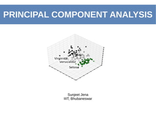
PRINCIPAL COMPONENT ANALYSIS
Sunjeet Jena
IIIT, Bhubaneswar

● What is PCA?
● Application to Different Fields
● Why PCA?
● Intuition
● Mathematics behind it
● Application to IRIS-Dataset
● Some Limitations of PCA
CONTENTS

● Principal component analysis (PCA) is a statistical
procedure that uses an orthogonal transformation to
convert a set of observations of possibly correlated
variables into a set of values of linearly uncorrelated
variables called principal components. (Source: Wikipedia)
● PCA was invented in 1901 by Karl Pearson, as an
analogue of the principal axis theorem in mechanics; it
was later independently developed (and named) by
Harold Hotelling in the 1930s.
WHAT IS PCA?

● Machine Learning and Image Recognition.
● Image Processing
● Data Clustering
● Dimentionality Reduction
● Data Visualization
APPLICATIONS to VARIOUS FIELDS

● PCA is mostly used as a tool in exploratory data
analysis and for making predictive models.
● It lessens the variables while computing the data and
therefore saves alot of computational power and time
without hampering the actual data much.
● It reduces the dimentionality of data for visualization.
● One of the efficient methods used for clustering of
similar data points.
WHY PCA?

INTUITION
Key Points:
➔ The 'x' represents a 2-dimensional data.
x1
x2

INTUITION
Cluster 1Cluster 1
Cluster 2
Key Points:
➔ The 'x' represents a 2-dimensional data.
➔ There are two clusters 1 and 2
➔ We want to reduce it to a one-dimensional sub-space

INTUITION
Key Points:
➔ The Straight Line Represents a Unit Vector 'U1'.
➔ The Data is projected on the Unit Vector 'U1'.
➔ The projected data has a large variance.
Cluster 1
Cluster 2
U1

INTUITION
Key Points:
➔ The Straight Line Represents a Unit Vector 'U1'.
➔ The Data is projected on the Unit Vector 'U1'.
➔ The projected data has a large variance.
Cluster 1 of
Original
Dimensionality
Cluster 2 of
Original
Dimensionality
Cluster 2 of reduced dimensionality
Cluster 1 of reduced dimensionality
U1

INTUITION
Key Points:
➔ The Straight Line represents a unit vector 'U2'.
➔ The data is projected on the Unit Vector.
➔ The variance of the projected data is small compared
to the previous slide.
Cluster 1 of
Original
Dimensionality
Cluster 2 of
Original
Dimensionality
U2

INTUITION
Key Points:
Cluster 1 of
Original
Dimensionality
Cluster 2 of
Original
Dimensionality
Cluster 2 of
Reduced
Dimensionality
Cluster 1 of
Reduced
Dimensionality
U2

INTUITION
Key Points:
So how do we find the Unit Vector where we can get
the highest variance of the projected data with?
Cluster 1 of
Original
Dimensionality
Cluster 2 of
Original
Dimensionality
Cluster 2 of
Reduced
Dimensionality
Cluster 1 of
Reduced
Dimensionality
U2

● Suppose we are given dataset {x (i) ; i = 1, . . . , m} with m
examples.
● There are n features/attributes for the each of the examples.
● So, x (i) R(n) for each i (n<<m)∈
● We want to reduce it to a one-dimensional sub-space with
largest variance of the data-set.
MATHEMATICS BEHIND IT

Before we apply PCA we need to pre-process the data to normalize its
mean and variance. The steps followed are:
Zero Out The Mean
Rescale each coordinate
to have unit variance.
So after we have normalized the data, whats next?

● Now, we need to find the Unit Vector along which the data can
be projected having the highest variance.
● Let 'u' be a unit vector.
● So given a Unit vector 'u' and a point 'x', the length of the
projection of x onto u is given by x(T)u {Meaning x Transpose
multiplied with u}.
● If x(i) is a point in our dataset (one of the crosses in the plot),
then its projection onto u (the corresponding circle in the figure)
is distance x(T)u from the origin.

Now to Maximize the variance of the projections, we would like to choose a unit-
length 'u' so as to maximize:
Average Distance of projected data from the origin
We know that we want to maximize the above eqauation and the only variable in it is
Unit Vector 'U' and therefore we need to maxmize it w.r.t to 'U'. So how do we do that?

● We have to keep in mind that one of the constraints we have is 'U' has be a Unit
Vector thus its magnitude should always be 1 i.e. ||u||=1.
● We need to maximize our equation based on this constraint.
● A quick reminder that of EigenValues and EigenVectors:
If A is a square matrix and if it satisfies the following equation:
AxU=LxU
then L is the eigenvalue of A and U is the eigenvector of A.
● There can be multiple solutions to the above equation and the Principle Eigenvector
of A would be corresponding to the highest Eigenvalue.

● Taking the Largangian we get:
L=Lagrange Multiplier
E
● Apply Lagrange Method of Optimization to find the solution(Maximizing the
distance of projected points from origin).

● Now when we equate above equation to zero we get:
Taking Derivative With Respect to 'u.'
This equation looks similar to what we had seen while we
revised EigenValues and Eigen Vectors.
● If we compare the above equation with what we got while we revised EigenVector and
Eigen Value, then it is seen that 'U' has to be the Eigen Vector of 'E' with a constraint
that ||u||=1.
● We also need to keep in mind that for dimensionality reduction of data to one-
dimension we need to consider the principle EigenVector of 'E'.
Solve this a an EigenValue Problem

● So, to summarize, we have found that if we wish to find a 1-
dimensional subspace with to approximate the data, we should
choose 'u' to be the principal eigenvector of E.
● So the Steps are:
1.Normalize the given data.
2.Maximize the distance of projected data onto the Unit Vector using Lagrangian
Optimization.
3.Find the Principle EigenVector which would satisfy the gradient of Lagrangian with
respect to 'u'.
4.The new data can be represented as:

● More generally, if we wish to project our data into a k-
dimensional subspace (k < n), we should choose u1, . . . ,
uk to be the top k eigenvectors of E.
● By top k Eigenvectors we mean the EigenVector
corresponding to the 'k' largest EigenValues.
● The new data therefore corresponds to:
● The vectors u1 , . . . , uk are called the first
k principal components of the data.

1.Normalize the given data.
2.Maximize the distance of projected data onto the Unit Vector using Lagrangian
Optimization.
3.Find the top 'k' EigenVector which would satisfy the gradient of Lagrangian with
respect to 'u'.
4.The new data can be represented as:
● So to get the dimensionality reduction to a k-dimensional
sub-space:

● What is IRIS Dataset?
The Iris flower data set or Fisher's Iris data set is a multivariate data set
introduced by Ronald Fisher in his 1936 paper The use of multiple
measurements in taxonomic problem.The data set consists of 50 samples
from each of three species of Iris (Iris setosa, Iris virginica and Iris
versicolor). Four features were measured from each sample: the length
and the width of the sepals and petals, in centimetres.(Source:Wikipidia)
APPLICATION TO IRIS DATA SET
IRIS SETOSA IRIS VERSICOLOR IRIS VIRGINICA

DATA SET
Sepal length Sepal Width Petal Length Petal Width Species
4.3 3.0 1.1 0.1 I. setosa
4.5 2.3 1.3 0.3 I. setosa
4.7 3.2 1.3 0.2 I. setosa
4.9 2.4 3.3 1.0 I. versicolor
5.0 2.0 3.5 1.0 I. versicolor
5.0 2.3 3.3 1.0 I. versicolor
5.8 2.7 5.1 1.9 I. virginica
6.0 2.2 5.0 1.5 I. virginica
6.2 3.4 5.4 2.3 I. virginica
Source:Wikipedia

Applying Principle Component Analysis using all features:
The above clustering diagram has been obtained using the Python library
“scikit-learn” which is an open-source library used for modelling PCA.
Source: http://scikit-learn.org/stable/auto_examples/decomposition/plot_pca_iris.html

Applying Principle Component Analysis using only two features:
Source: http://scikit-learn.org/stable/auto_examples/datasets/plot_iris_dataset.html

● Dimension reduction can only be achieved if the original
variables were correlated. If the original variables were
uncorrelated, PCA does nothing, except for ordering them
according to their variance.
● The directions with largest variance are assumed to be of most
interest.
● PCA is based only on the mean vector and the covariance
matrix of the data. Some distributions are completely
characterized by this, but others are not.
SOME LIMITATIONS Of PCA

SOME LIMITATIONS OF PCA
● Limitation of PCA can be seen with MNIST Dataset.
● So what is MNIST Dataset?
The MNIST database (Mixed National Institute of Standards and
Technology database) is a large database of handwritten digits that is
commonly used for training various image processing systems.The
database is also widely used for training and testing in the field of
machine learning. (Source: Wikipedia)
➔ The MNIST database contains 60,000 training images and 10,000 testing images.
➔ Each data is a 28x28 Pixel Image.
● PCA is applied to the MNIST Dataset considereing each pixel value as a
dimension and therefore each data is represented in 784 dimensional graph .
PCA reduces it to a 2-dimensional sub-space.

SOME LIMITATIONS Of PCA
We can't figure
out the
clusters if the
labels are
removed.

Introduction to Principle Component Analysis

Recommended

Recommended

More Related Content

What's hot

What's hot (20)

Similar to Introduction to Principle Component Analysis

Similar to Introduction to Principle Component Analysis (20)

Recently uploaded

Recently uploaded (20)

Introduction to Principle Component Analysis