20_Baxter pompei ref

239
Archeologia e Calcolatori
19, 2008, 239-256
NOTES ON THE STATISTICAL ANALYSIS
OF SOME LOOMWEIGHTS FROM POMPEII
1. Introduction
Within the archaeological record there are many types of artefacts that
attract very little attention even in the specialist literature. Generally this is
because they are utilitarian items whose basic forms remain unchanged for
centuries. As such they are neither useful for dating purposes, nor suf�ciently
attractive in themselves to generate interest from an art historical point of
view.Yet even these apparently mundane items can provide useful information
about the people who made and used them if analysed appropriately. It is the
aim of the present paper to take just such an apparently unpromising item,
and show how statistical analysis can provide useful information. The type
chosen to illustrate this here is the loomweight, using data derived from the
excavations in Insula VI.I, Pompeii, but the methodological approach could
be applied to many other apparently mundane and “uninteresting” types.
Initial statistical analysis on the weights of the loomweights was under-
taken in the �eld. Somewhat to our surprise the distribution of the weights
appeared to be distinctly bi-modal.Subsequent analysis,reported here,appears
to con�rm this and, additionally, suggested patterns in the data associated with
the shapes of the base and top of the loomweights. Full interpretation of the
results in cultural and archaeological terms has to await the full analysis of
the stratigraphy, but it is possible to advance some preliminary conclusions
and these are offered in our concluding discussion. The focus of the present
paper is on the statistical methods used to reach our conclusions about the
loomweights. The aims of the paper may be summarised as follows:
a) The use of simple, and not so simple, statistical techniques is illustrated on
a body of material that many might regard as unpromising, with the aim of
showing what can sometimes be “teased out” of such data.
b) Rather more analyses than are strictly necessary to make our case are
shown.This is deliberate.Apart from illustrating how our thinking progressed
we want to illustrate different methods in suf�cient detail to provide ideas
for other researchers faced with similar data for other classes of object. This
is related to the next aim.
c) All our analyses were undertaken using the powerful open source R system.
This will be familiar to many readers of «Archeologia e Calcolatori», but per-
haps not all. For the bene�t of the latter, the appendix discusses the functions
used in suf�cient detail to allow interested readers to emulate our analyses.
Mathematical detail is deliberately avoided, but references are provided that
direct the reader to the necessary statistical theory.

M.J. Baxter, H.E.M. Cool
240
d) Finally some preliminary interpretations are offered,some rather specu-
lative. This paper is mainly about identifying patterns for a particular class of
artefact.We are not aware that loomweights have been studied in the detail we
go into before, so the paper may be of interest for this reason alone. Ultimately,
however, it is the interpretation of the patterns observed that is important.
2. Data
Loomweights were used on warp-weighted looms to hold the warp
thread under tension (Wild 1970, 61-65; Ciarallo, De Carolis 1999, 146,
n. 140). Functionally their most important feature is their weight, as the front
and back threads need to be kept under the same tension (Hoffman 1964,42).
In the archaeological literature there is a tendency to describe any weight with
a perforation near the apex as a loomweight. Some authorities have argued
against this, noting that they could have been used for other purposes and
that much stricter criteria need to be in place before such an identi�cation can
be made (see for example Castro Curel 1985). Fortunately the examples in
this study can be identi�ed as loomweights with some degree of certainty as
they are of the same type as those found in situ with the carbonised remains
of what was interpreted as a loom in a portico of a house at Herculaneum
(Maiuri 1958, 430).Whilst noting that some could have had other purposes,
in this paper the objects will be referred to as loomweights for convenience
so that the term“weight”may be reserved for use when aspects of how much
the items weighed are being discussed.
The data in this paper are derived from examples recovered during the
excavation of Insula VI.1 by the Anglo-American Project in Pompeii. This
insula lies by the Herculaneum Gate and was one of the earliest areas stripped
of volcanic debris in the late eighteenth century. It includes the famous House
of the Surgeon (Casa del Chirurgo) as well as the House of the Vestals (Casa
delle Vestali). Some of the wall and �oor decorations were removed when
it was originally excavated. The erosion it has suffered in the two centuries
since then, including damage caused during the Second World War when it
was hit by a bomb dropped by the Allies, means that very few of the original
�oor surfaces present at the time of the eruption in AD 79 now survive. This
has enabled the project to excavate the insula within and around the stand-
ing walls to uncover its history from the fourth century BC when occupa-
tion commenced, up to the eruption (for a general account of the project see
Jones, Robinson 2004a; Jones, Robinson 2004b provide a more detailed
consideration of one area of the insula).
The excavations were concluded in 2006 and post-excavation analysis is
now ongoing. During the 2007 season of work, 150 complete and fragmentary
�red clay weights were recorded from the insula together with four from trial

Notes on the statistical analysis of some loomweights from Pompeii
241
excavations undertaken by the project in Insula V.2 in 2005. Most of the loom-
weights were of the typical truncated pyramidal form with a perforation run-
ning through the upper part (Fig. 1, n. 142).A small number had a pronounced
square outline with a rectangular cross-section (Fig. 1, n. 116).A minority had
been decorated generally with one or more circular dimples impressed or cut
into the upper surface, but cross patterns and stamps were also present. The
decoration on the upper part was always made before �ring.Occasionally there
were hollows on the bases but these had been cut after the item had been �red.
Loomweights such as these were very common in the Mediterranean area for
a long period. In Greece they are recorded from at least the eighth century BC
(Davidson, Thompson 1943, 73), in Iberia they are recorded from the sixth
century BC onwards (Castro Curel 1985, 232, �g. 3) whilst in Languedoc
examples have been found from the fourth century BC (de Chazelles 2000,
121). Their use continued into the Roman Imperial period (Fig. 1).
Though loomweights were found throughout the insula, they showed
a marked concentration in the area occupied by the Casa del Chirurgo.
Stratigraphic information is not yet available for all parts of the insula, but
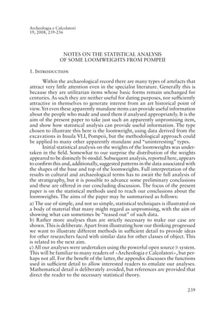
Fig. 1 – Examples of the ceramic loomweights discussed. Diagram A (not
to scale) shows how the height was measured using the offset method.

242
fortunately the analysis for the Casa del Chirurgo is almost complete. This
indicates that the loomweights were being regularly recovered throughout
the stratigraphic sequence, from the earliest contexts up to those of the mid
�rst century AD.
The protocol followed in recording them was that the loomweight was
measured on scales that were accurate within 2 grams. The height and the
measurements of the base and top were recorded to the nearest millimetre.
Some of the tops and bottoms had rounded junctions with the sides rather
than the edge being sharp. In such cases it was not always easy to see precisely
where the edge should be measured. This problem was most marked on the
tops of the smaller weights with the larger ones tending to have more sharply
marked edges; but sharp edges did occur on small weights and rounded ones
on larger. Given this uncertainty, if the top (or bottom) appeared to be square
only one measurement was taken. If the section appeared to deviate from the
square two measurements were taken.
After the initial recording when preliminary analysis suggested the weight
of the pieces was bimodal, the height of all the complete loomweights was re-
measured using an offset method (Fig. 1,A) to ensure consistency.Again it was
not always possible to be entirely accurate as some bases were slightly rounded
and did not sit �at. It will be appreciated that there is measurement error on all
aspects of the data, but in the worst case scenario we estimate that this should
be no greater than approximately 3 millimetres or grams. In what follows
only the 95 complete loomweights are discussed. They were considered to be
complete if they retained all of their edges. Minor chipping was ignored.
3. Statistical Analysis: results
3.1 One-dimensional analyses of weights
The histogram is a common choice for initial exploration of continu-
ous data. The left-hand panel Fig. 2 shows our �rst attempt at this. There is
apparently nothing unusual about the data, apart from some untypical small
and large weights.
Default interval widths (bin-widths) were used giving rise to eight bins
of equal width, 100 g. Our experience is that defaults in software often tend
to over-smooth data. The right-hand panel of Fig. 2 shows a histogram using
subjectively determined bin-widths of 25 g, with a kernel density estimate
(KDE) superimposed.
This �gure suggests that the data are bimodal. Before seeking an ar-
chaeological interpretation for this, con�rmation of the“reality”of the effect
was sought. There are six unusual weights, one very small and �ve greater
than 400 g. For some subsequent analyses these are removed, and we shall
refer to this as the “modi�ed” data set.

243
The KDE suggests that the modi�ed data, excluding the six extreme
values, can be approximated well by a mixture of two normal distributions.
The software used to do this allows for a test of the number of normal com-
ponents in the mixture, and provides estimates of the means and standard
deviations of the components as well as the graphical representation shown
in Fig. 3, which is based on the modi�ed data.
The analysis con�rms that a two-component normal mixture is optimal,
and that these can be taken to have equal standard deviations, estimated as
41.5. The estimated means are 166.0 and 300.7, with 45 and 44 cases clas-
si�ed to the two groups. Cases with weights 230 g or less are assigned to the
�rst group and cases with 239 g or more to the second group; the anti-mode
in Fig. 3 is at about 235 g. This gives groups of size 46 and 49 if the rule is
used to classify all the weights.
3.2 Two-dimensional analyses: weight and height
A quick way to look at the data (using all the loomweights) is to look at
all possible bivariate plots, as in Fig. 4. In general the variables are positively
correlated,as we would expect,though not strongly so in some cases.The largest
correlation in the plots shown,of r = 0.82,is between weight and height,and for
further analysis this will be the initial focus of attention (base area has a higher
correlation which we discuss later). The patterns evident in the maximum and
minimum dimensions of the top and bottom are also discussed later.
Fig. 2 – Two histograms using different bin-widths that show the distribution of weights of loom-
weights from Pompeii. That to the right suggests the distribution is bimodal.
1
0 200 400 600 800
0.0000.0010.0020.003
weight
0 200 400 6000.0000.0010.0020.0030.0040.005
weight
Fig. 2 – Two histograms using different bin-widths that show the distribution of weights of
loomweights from Pompeii. That to the right suggests the distribution is bimodal.
100 150 200 250 300 350
0.0010.0020.0030.0040.005
density
Density
Fig. 3 – An estimated two-component normal mixture for the weights of the loomweights.

244
Fig. 5 is similar to the right-hand panel of Fig. 2 but for height (using
bin-width 5 and bandwidth 18). This also shows bimodality. Fig. 6 is a plot
of height against weight using the modi�ed data, labelled according to the
classi�cation suggested by the mixture analysis for weight. Some weights could
be reclassi�ed to group 2 on the visual evidence. We return to this later.
It is possible to �t two-dimensional KDEs to the modi�ed data and
display the results in various ways, as in Fig. 7, which all suggest two main
concentrations of data. Usually only one of these plots would be needed, but
they are all shown for illustration. The plot of choice can be customised if
desired. In Fig. 8, for the contour plot, the limits of the axes have been changed;
the number of contour levels has been modi�ed and labelling of the levels
removed; and the contours have been overlaid on the plot of the data.
Visually the plots suggest a mixture of two bivariate normal distribu-
tions. Two (ellipsoidal) normal distributions of equal volume and shape, but
different orientations, are adequate to describe the data. Different methods
of displaying the results are shown in Fig. 9.
The upper left plot is of the Bayesian Information Criterion for different
possible models, and is used to select the number and type of normal distribu-
tions �tted. The classi�cation plot suggests, visually, that there are possibly
three points allocated to the lower-left group that might better sit with the
upper-right group.The larger dots in the classi�cation uncertainty plot identify
cases for which the classi�cation is least certain; there are �ve “intermediate”
cases here. The ellipses on the two plots correspond to the covariances of the
components. By comparison with Fig. 6, there is a slight change (three cases)
from the classi�cation obtained when only weight is used.
1
0 200 400 600 800
0.00
weight
0 200 400 600
0.00
weight
Fig. 2 – Two histograms using different bin-widths that show the distribution of weights of
loomweights from Pompeii. That to the right suggests the distribution is bimodal.
100 150 200 250 300 350
0.0010.0020.0030.0040.005
density
Density
Fig. 3 – An estimated two-component normal mixture for the weights of the loomweights.
Fig. 3 – An estimated two-component normal mixture
for the weights of the loomweights.

245
2
weight
40 80 120 10 30 20 40 60
0400
4080120
height
Topmax
2040
1030
Topmin
Bottommax
20406080
0 400
204060
20 40 20 40 60 80
Bottommin
Fig. 4 – A “pairs” plot for six variables that characterise the loomweights, showing all
possible bivariate plots. The upper triangle of plots is the same as the lower triangle, except
that axes are interchanged. Treating the base and apex of the weights as rectangular, Topmax
is the length of the larger sides of the rectangle at the apex and Topmin relates to the smaller
side. Bottommax and Bottommin refer to similar dimensions for the base.
Fig. 4 – A “pairs” plot for six variables that characterise the loomweights, showing all possible
bivariate plots. The upper triangle of plots is the same as the lower triangle, except that axes are
interchanged. Treating the base and apex of the weights as rectangular, Topmax is the length of the
larger sides of the rectangle at the apex and Topmin relates to the smaller side. Bottommax and
Bottommin refer to similar dimensions for the base.
40 60 80 100 120
0.0000.0050.0100.0150.0200.025
height
ig. 5 – A histogram for the heights of the loomweights with a kernel density estimate
uperimposed.
0100110120
x
x
x
x
x
xx x
x
x
x
x
x
x
x
x xx
xx
x
x
x
x
x
x
x
x
x
x
o
x
x
x
x
o
x
xo
x
x
x
o
40 60 80 100 120
0.0000.0050.0100.0150.0200.025
height
Fig. 5 – A histogram for the heights of the loomweights with a kernel density estimate
superimposed.
100 150 200 250 300 350
60708090100110120
weight
height
o
x
x
x
o
x
x
xx
o
x
x
x
x
x
x
o
x
o
x
o
o
x
x
o
x
x x
o
x
xx
x
x
x
o
o
o
o
o
o
x
o
o
o
x
x
x
x
o
x
x
x
x
o
o
o
o
x
x
o
o x
x
o
x
o
o
o
o
x
o
o o
o
x
o
o
o
o
o
o
o
o
x
o
o
x
o
Fig. 6 – A plot of height against weight, with cases labelled by the classification sug
the mixture analysis.Fig. 5 – A histogram for the heights of the
loomweights with a kernel density estimate
superimposed.
Fig. 6 – A plot of height against weight, with
cases labelled by the classi�cation suggested by
the mixture analysis.

246
100 200 300
6080100120
weight
height
150 200 250 300 350
6080100
weight
height
kdeest
Y
Z
weight
height
100 200 300
6080100120
Fig. 7 – Different ways of displaying the relationship between height and weight. The raw
data is to the upper-left; an image plot is to the upper-right; a perspective plot is to the lower
left; a contour plot is to the lower-right.
100 200 300 400
406080100120
weight
height
Fig. 8 – A customised version of the contour plot shown in Fig. 7.
Fig. 7 – Different ways of displaying the relationship between height and weight.
The raw data is to the upper-left; an image plot is to the upper-right; a perspective
plot is to the lower left; a contour plot is to the lower-right.
100 200 300
6080100120
weight
height
150 200 250 300 3506080100
weight
height
kdeest
Y
Z
weight
height
100 200 300
6080100120
Fig. 7 – Different ways of displaying the relationship between height and weight. The raw
data is to the upper-left; an image plot is to the upper-right; a perspective plot is to the lower
left; a contour plot is to the lower-right.
100 200 300 400
406080100120
weight
height
Fig. 8 – A customised version of the contour plot shown in Fig. 7.
Fig. 8 – A customised version of the contour plot
shown in Fig. 7.

247
5
2 4 6 8
-1950-1850-1750
number of components
BIC
100 200 300
6080100120
Classification
100 200 300
6080100120
Classification Uncertainty
100 200 300
6080100120
Density Contour Plot
Fig. 9 – Assuming that the height/weight data can be modelled using a mixture of bivariate
normal distributions, this figure shows different ways of displaying the results.
1.0 1.5 2.0 2.5
1.01.21.41.61.82.02.2
bottom (max/min)
top(max/min)
ooo
o
o
o
o
o
o
o
o
o
o oo
o
oo oo
o
o
o
o o
o
o
o
oo oo
o
oooo
o
o
o
o
o
o o
o
o
o
o
o
oooooooooooooooooooooooooooooooooooo
o
o
o
o
o
o
o o
oo
Fig. 9 – Assuming that the height/weight data can be modelled using a
mixture of bivariate normal distributions, this �gure shows different ways
of displaying the results.
3.3 Other dimensions
Returning to Fig. 4 it can be seen that the plots of the maximum and
minimum dimensions for the bottoms and tops of the loomweights show
distinctive linear features. These correspond to loomweights where the top
or bottom was square. For non-square bottoms the minimum difference be-
tween the two sides was 2 mm – in two cases – but usually exceeded 5 mm.
For non-square tops, which are smaller than the bottoms, there were more
instances of small differences in the dimensions, including one of 1 mm.
Fig. 10 shows a plot of the maximum to minimum ratios for the tops
against those for the bottoms.The plot has been jittered – that is each point is
displaced by a small random amount – so that the“blob”in the (1, 1) position
corresponds to the 52 of the sample with square tops and bottoms.
The 8 cases vertically above the (1, 1) position have square bottoms and
rectangular tops, with the reverse the situation for the 13 cases horizontally
along from the (1, 1) co-ordinate. The dashed line is that on which points
would fall (ignoring jittering) if the ratios were the same for both top and
bottom. There are 22 loomweights that have neither a square bottom nor

248
top. More than half are close enough to this line to suggest that a deliberate
attempt might have been made to have the tops and bottoms exactly identical
in shape. The dotted line corresponds to the situation where the ratio for the
bottom is 1.5 times that for the top. Most of the remaining cases lie close to
this line (we emphasize that, given the numbers involved, these observations
are tentative).
If the ratio of the ratios is computed it should be close to 1 if the tops
and bottoms have (almost) the same shape; 65/95 lie between 0.95 and 1.05,
which implies that 13/22 of the loomweights noted above are close to having
rectangular tops and bottoms of exactly the same shape.
Analyses so far suggest that, on the basis of weight and height, it is
possible to divide the loomweights into two size classes. To relate this, if
possible, to the shape information discussed above a tentative typology can
be suggested which is:
Type 1 = square bottom and top (e.g., Fig. 1, n. 142);
Type 2 = rectangular (non-square) bottom and top of similar relative dimen-
sions;
Type 3 = square bottom and rectangular top;
Type 4 = square top and rectangular bottom (e.g., Fig. 1, n. 116);
Type 0 = other.
There is some suggestion in Fig. 11 that the heaviest of the weights (about >
375 g) tend to be of Type 1.
An alternative way to look at the data is to cross classify by size. For
the present purposes we slightly modify the classi�cations suggested by the
mixture models, to take into account visual evidence, and do not separate
out the unusual values. Call these classes “Small” and “Large”; the modi�ed
classi�cation is shown in Fig. 12. The cross classi�cation gives the Tab. 1.
A conventional chi-squared test gives X2
= 15.28 on 4 D.F. with a p-value
of 0.0041 (using Monte Carlo simulation give a p-value of 0.001).There is thus
a clear association between the size-based and type-based classi�cations.
The type-based classi�cation was derived on the basis of aspects of shape
(of bottoms and tops) using ratios that eliminate size effects. That is, the two
classi�cations, while related, were derived independently. The most obvious
feature of the table is that all but one of the Type 4 loomweights (square top,
rectangular bottom) is“large”.Type 0 tends to be“small”but there are relatively
few of them.There are more largeType 1 weights than small ones,but given the
different groups sizes this is not unexpected; under the hypothesis of no associa-
tion about 30 would be expected, which differs little from the observed 32.
The chi-squared test can be insensitive to interesting features of the
data. As noted from Fig. 11, a disproportionate number of the larger weights
are of Type 1 (and possibly 4). This can be seen graphically in Fig. 13. The
horizontal dashed line, at 0.55, is the proportion of loomweights with square

249
5
100 200 300 100 200 300
Fig. 9 – Assuming that the height/weight data can be modelled using a mixture of bivariate
normal distributions, this figure shows different ways of displaying the results.
1.0 1.5 2.0 2.5
1.01.21.41.61.82.02.2
bottom (max/min)
top(max/min)
ooo
o
o
o
o
o
o
o
o
o
o oo
o
oo oo
o
o
o
o o
o
o
o
oo oo
o
oooo
o
o
o
o
o
o o
o
o
o
o
o
oooooooooooooooooooooooooooooooooooo
o
o
o
o
o
o
o o
oo
Fig. 10 – A plot of the maximum to minimum ratio of
the tops of the loomweights against a similar ratio for
the bottom of the loomweights.
Fig. 10 – A plot of the maximum to minimum ratio of the tops of the loomweights against a
similar ratio for the bottom of the loomweights.
0 200 400 600
406080100120
weight
height
4
1
1
3
0
0
4
01
2
4
3
4
4
4
3
1
1
4
1
2
1
0
1
4
0
2
3 1
1
4
42
4
1
1
1
2
2
3
3
2
1
4
2
3
3
2
2
1
1
1
1
1
1
1
1
1
1
1
1
1
1
1
1 1
1
1
1
1
1
1
1
1
1
1
1
1 1
1
1 1
1
1
1
2
0
0
2
0
1
2
0
4
1
Fig. 11 – A plot of height against weight, labelled according to the shape typology suggested
by Fig. 10.Fig. 11 – A plot of height against weight, labelled according to the shape
typology suggested by Fig. 10.

250
tops and bottoms. Between about 100 g and 280 g (only one weight is less
than 100 g) the proportion of Type 1 loomweights greater than any given
weight is not markedly different from the proportion in the sample. As the
weight threshold is increased beyond 280 g the proportion of Type 1 weights
increases, the non-monotonic nature of the increase at larger weights being
attributable to Type 4 weights. For example, 72% of the 25 weights greater
than or equal to 300 g are Type 1 and 92% are Type 1 or 4.
Some thought was given to the problem of predicting weight from other
variables that might be present on damaged loomweights (of which we have
58). A height measurement is not usually available for these, but 34 have
complete bases, and consideration was given to using these for prediction, in
the form of base area.
For the data set of complete loomweights the correlations of base area
and height with weight are 0.88 and 0.82 respectively; for the modi�ed com-
plete data the correlations are 0.73 and 0.84, suggesting that the unusual data
are particularly in�uential for the base area data. Excluding the unusual data
the correlation of 0.73 implies that about 50% of the variation in weight can
be “explained” by base area (assuming a linear model holds), so that predic-
tions will not be very precise.
This is con�rmed by Fig. 14, for the modi�ed data, which shows a plot
of weight against base area, with the linear regression line, and a non-linear
(loess) smoother superimposed. The latter is very close to the regression line,
suggesting that a linear model is acceptable, but the spread of weight values
at any give base area is evident. Formal calculation of prediction intervals
con�rms that they are wide within the relevant base area range, so the aim of
prediction from damaged weights using base area was not pursued.
4. Discussion
As mentioned in the introduction, the analysis of the stratigraphy, pot-
tery etc. has not advanced suf�ciently for it to be possible to date the majority
of the loomweights by their context. In the case of those from the Casa del
Chirurgo it is possible to isolate small groups from contexts of different dates.
There is a group of �ve from features and levels that pre-date the building of
Tab.1 –A cross-classi�cation of size by
shape type, based on the classi�cations
described in the text.
Size Type Total
0 1 2 3 4
Large 2 32 4 4 12 54
Small 7 20 9 4 1 41

251
1000 1500 2000 2500 3000
100150200250300350
base area
weight
Fig. 14 – A plot of weight against base area, for the modified data that omits unusual data. The
solid line is a fitted linear regression used to investigate how well base area can predict height
if the loomweight is incomplete. The dashed line is a non-linear smoother. It is close to the
regression line, suggesting that more complicated methods of prediction are not required.
Fig. 1 – Examples of the ceramic loomweights discussed. Scale 1:1. Diagram A (not to scale)
shows how the height was measured using the offset method.
Fig. 15 – A kernel density plot of the modified dataset labelled with the Casa del Chirugo
groups summarised in Table 1.
Fig. 14 – A plot of weight against base area, for the
modi�ed data that omits unusual data. The solid line
is a �tted linear regression used to investigate how
well base area can predict height if the loomweight is
incomplete. The dashed line is a non-linear smoother.
It is close to the regression line, suggesting that more
complicated methods of prediction are not required.
7
0 200 400 600
406080100120
weight
height
o
x x
x
o
x
xxx
o
x
x
x
x
x
x
x
o
x
o
x
o
o
x
x
o
x
x x
o
x
xx
x
x
x
x
o
o
o
o
o
o
x
o
o
o
o
x
x
x
x
o
x
x
x
x
o
o
x
o
x
x
o
x x
x
xx
x
x
o
o
o
o
x
o
o o
x
x x
o
o
o
o
oo
o
o
x
oo
x
x
Fig. 12 – Similar to Fig. 6 but using all the data and with a modified size classification.
0 100 200 300 400
0.00.20.40.60.81.0
weight
proportionoftype1>weight
Fig. 13 – A graphic that suggests that Type 1 loomweignts, with square tops and bottoms, are
disproportionately likely to be of a heavier weight.
Fig. 12 – Similar to Fig. 6 but using all the data
and with a modi�ed size classi�cation.
7
0 200 400 600
40
weight
o
Fig. 12 – Similar to Fig. 6 but using all the data and with a modified size classificatio
0 100 200 300 400
0.00.20.40.60.81.0
weight
proportionoftype1>weight
Fig. 13 – A graphic that suggests that Type 1 loomweignts, with square tops and b
disproportionately likely to be of a heavier weight.Fig. 13 – A graphic that suggests that Type 1
loomweights, with square tops and bottoms,
are disproportionately likely to be of a heavier
weight.
the house in c. 200 BC. Five were also found in a pit dug to extract building
material to extend the triclinium. This was re-�lled with domestic rubbish
dated to about 100 BC. Finally nine can be dated to the mid �rst century AD

252
as they were recovered from make-up and levelling layers below the �nal
�oors in the Casa del Chirugo, and in one case was incorporated into such a
�oor. This phase of rebuilding is believed to have been undertaken between
the earthquake, conventionally dated to AD 62, and the eruption in AD 79.
These are summarised in Tab. 2 according to the weight and shape types
de�ned above.
We stress that this is a very small sub-set of the data but as can be seen
there does appear to be a progression from small to large loomweights with
time and a suggestion that what might be called the “non-standard” shapes,
i.e. the Type 2 ones with the rectangular tops and bottoms of similar dimen-
sions, and the ones that did not �t into any of the four main types (classi�ed
as Type 0), were of early date.
Amongst the Group 2 loomweights (of c. 100 BC) there is one large
outlier (467 g).The Group 3 loomweights (mid �rst century AD) include three
outliers; the miniature one of 15 g and two large ones (564 and 634 g). The
examples which fall into the modi�ed data set are plotted in Fig. 15 (the top
left plot of Fig. 7) with the points labelled according to which Group they fall
into. As well as labelling the weight axis by modern gram measures (bottom
edge), it has been labelled according to Roman unciae measures along the top
edge. The problems of establishing the precise weight of the Roman pound
(libra) have been rehearsed by Crawford. Various weights have been calcu-
lated ranging from 320 g to 327.45 g (Crawford 1974, 591 and addenda).
The higher level is normally preferred (e.g. RIB II.2, 1-2; DNP 5.147). Here
we follow Crawford in using a measure of 27 g for one uncia (there were 12
unciae to the libra).
It is known that the Roman pound of this weight was in use in the mid
�rst century in Pompeii because a steelyard has been found there with an
inscription that certi�ed it was in accordance to the weight standard estab-
lished in Rome in the year AD 47 by the aediles Marcus Articuleianus and
Gnaeus Turranius (Ward-Perkins, Claridge 1976, 249, n. 248; Ciarallo,
De Carolis 1999, 299, n. 370). The unciae scale would thus be suitable
for the loomweights of Group 3. In the third century BC, however, it would
appear that what constitutes a Roman libra was not so stable. At different
points during that century the Roman aes coinage was based on both what
Group Date Small Large Total
0 2 3 1 1 3 4
1 Pre c. 200 BC 2 2 - 1 - - - 5
2 c. 100 BC - - - 3 2 - - 5
3 c. 62-79 AD - - 1 3 3 1 1 9
Total 2 2 1 7 5 1 1 19
Tab. 2 – Independently dated loomweights from the Casa del Chirugo.

253
was to become the accepted Roman pound and on the Oscan pound of c.
273 g (Sutherland 1974, 25-27), and Roman measures were not dominant
through Italy as they were to be three centuries later. It is thus possible that
for the Pompeian makers and users of the Group 1 loomweights, an uncia
weighed something else (Fig. 15).
Allowing for these problems with calculating the Roman libra, it is very
noticeable that the third century BC loomweights (Group 1) cluster between
4 and 6 unciae and the mid �rst century AD ones of Group 3 range between
6 and 12 unciae, possibly suggesting that their makers were working towards
producing loomweights of speci�c weights and that these changed with time.
Considerably more independent dating evidence is needed than that currently
available to us, but there is the possibility that the weight of the loomweights
might have chronological signi�cance at Pompeii. If there was a shift in the
size of the loomweights with time then other questions can be explored such
as whether there were changes in the nature of the textiles being produced.
The increasing standardisation of the shape with time might also point to an
increasing level of centralisation in the production of these artefacts.
If the pattern is reproduced elsewhere in the insula, loomweights may
move into the category of �nd that is chronologically sensitive and, as we
noted in the introduction, more attention is always devoted to such �nds.
More information about them is recorded when they are catalogued and
this allows more detailed analysis to be undertaken, so that the artefact can
contribute more fully to our understanding of the people who made and used
them. In preparing this paper, for example, we have been surprised at how
Fig. 15 – A plot of the modi�ed dataset labelled
with the Casa del Chirugo groups summarised
in Tab. 1.

254
often comparable loomweights have been published without their weights
being recorded, yet as we have shown weight is probably the most important
element to record.
Finally it is useful to re�ect in the light of this paper, that had the analy-
sis stopped after using the default software interval width for the histogram
shown in Fig. 2, we would not have uncovered the patterns within the data.
We hope that this will encourage others to go beyond the default choices
when they too have apparently unpromising datasets like this.
Acknowledgements
We are most grateful to Pietro Giovanni Guzzo, Antonio D’Ambrosio and all their
colleagues in the Soprintendenza Archeologica di Pompei for their continued support and
encouragement of the Anglo-American Project, and for the permission to work on the ar-
tefacts from the insula. The Anglo-American Project is directed by Rick Jones and Damian
Robinson and we thank them for inviting H.E.M. Cool to analyse the �nds. We are very
grateful to Damian and to Michael Anderson (Field Director) for discussions about this ma-
terial and for providing contextual information relating to the Casa del Chirurgo. A special
thanks goes to Kelly Leddington and Katie Huntley who were H.E.M. Cool’s assistants in
2007 and who recorded the loomweights. Ms Leddington and Ms Huntley were funded by
a grant from the Society of Antiquaries of London, and we are most grateful to the society
for their support. We also thank Jessica Billing, Sarah Lloyd and Stuart Ward (students at
the �eld school in 2007) who provided additional assistance. Penelope Walton Rogers most
kindly responded to our queries about the use of loomweights and pointed us to literature
we were unaware of.
Mike J. Baxter
Department of Physics and Mathematical Sciences
Nottingham Trent University
Hilary E.M. Cool
Barbican Research Associates
Nottingham
Appendix
Computational Details
R is a powerful open source statistical software system. Open source software is of
increasing interest in archaeology (Pescarin 2006); apart from being free, R has the additional
advantages that many statisticians would regard it as “state-of-the-art”, and it is regularly
updated. A good starting point is K. Hornik, The R-FAQ, available at http://cran.r-project.
org/doc/FAQ/. This is updated as newer versions of R become available, but the URL is a
constant. The FAQ includes information on how to obtain and install R, and lists some books
available about it.
R is currently the software of choice for many applied statisticians. A major strength
of R is that there are numerous packages developed by such statisticians that can be used for
a wide range of statistical analyses – many of them quite specialised. Packages not distributed
with R are readily downloaded.
For Fig. 2 the histograms were obtained using the truehist function from the MASS
package, associated with the book of Venables, Ripley (2002). This is plotted on a relative
frequency density scale, rather than a frequency scale. For the KDE and its superimposition on

255
the histogram, the code in Venables, Ripley (2002, 437) was emulated, using a subjectively
chosen bandwidth of 80. This is a bit less than that suggested by the Sheather-Jones estimate
(Sheather, Jones 1991) used in Venables and Ripley’s example.
For Fig. 3, version 3 of the mclust package was used, closely following the examples
in Fraley, Raftery (2006, 32-34). Particular use was made of the Mclust and mclustBIC
functions. This paper directs readers to sources that discuss the relevant statistical theory.
Venables, Ripley (2002, 437-442) also provide relevant code, partly to illustrate features
and functions available in R.
Fig. 4 used the pairs function; Fig. 5 is similar to the right-hand panel of Fig. 2; Fig. 6,
10-12 and 14 use the plot function with the text function used to control plotting symbols,
and the abline and lines functions used to superimpose lines of various kinds. In Fig.
10 the jitter function was used to accomplish jittering. In Fig. 14 the regression line was
computed using the lm function and added to the plot using abline; the loess smoother was
computed and superimposed following the code given in Venables, Ripley (2002, 230) using
the loess.smooth function..
Fig. 7 follows the example in the help �le for kde2d from the MASS package, using
n = 50 for the kde2d function and defaults for the image, persp and contour functions.
For Fig. 8, in kde2d, n = 100 was used with upper and lower limits for weight of 50 and 430,
and limits of 35 and 130 for height. These need to be set to be the same in the plot function
for weight against height. Compared to the contour plot in Fig. 7, more levels are used and
labelling of contour height is removed. In the contour function the argument add = TRUE
is used to overlay it on the previously created plot.
For Fig. 9 the Mclust and plot.Mclust functions from the mclust package were
used exactly as described in Fraley, Raftery (2006, 4-7).
Fig. 13 was produced using a function written by one of us (M.J.B.).
REFERENCES
Castro Curel C. 1985, Pondera, examen cualitativo, cuantitivo especial y su relación con el
telar con pesas, «Empúries», 47, 230-253.
Ciarallo A., De Carolis E. (eds.) 1999, Homo Faber: Natura, Scienza e Tecnica nell’antica
Pompei, Milano, Electa.
Crawford M.H. 1974, Roman Republican Coinage, Cambridge, Cambridge University
Press.
Davidson G.R., Thompson D.B. 1943, Small Objects from the Pnyx: I, «Hesperia», Supple-
ment VII, Athens.
de Chazelles Cl.-A. 2000, Eléments archéologiques liés au traitement des �bres textiles en
Languedoc occidental et Roussillon au cours de la protohistoire (VIe
-1er
s. av. n. è.), in
D. Cardun, M. Feugère (eds.), Archéologie des textiles des origines au Ve
siècle. Actes
du Colloque (Lattes 1999), Montagnac, Monique Mergoil, 115-130.
DNP = Der Neue Pauly, Stuttgart, Verlag JB Metzler.
Fraley C., Raftery A.E. 2007, MCLUST VERSION 3: An R package for normal mixture
modelling and model-based clustering (http://www.stat.washington.edu/www/research/
reports/2006/tr504.pdf).
Hoffman M. 1964, The Warp-weighted Loom, «Studia Norvegica», 14, Oslo.
Jones R., Robinson D. 2004a, Imperial Pompeii: a city of extremes, «Current World Archae-
ology», 4, 32-39.
Jones R., Robinson D. 2004b, The making of an elite house: the House of the Vestals at
Pompeii, «Journal of Roman Archaeology», 17, 107-130.
Maiuri A. 1958, Ercolano: Nuovi Scavi (1927-1958), Roma, Istituto Poligra�co dello
Stato.

256
Pescarin S. 2006, Open source in archeologia. Nuove prospettive per la ricerca, «Archeologia
e Calcolatori», 17, 137-155.
RIB II.2 = Collingwood R.G., Wright R.P., The Roman Inscriptions of Britain. Volume
II, Fascicule 2, Instrumentum Domesticum (personal belongings and the like), Stroud,
1991 (S.S. Frere, R.S.O. Tomlin eds.).
Sheather S.J., Jones M.C. 1991, A reliable data-based bandwidth selection method for kernel
density estimation, «Journal of the Royal Statistical Society B», 53, 683-690.
Sutherland C.H.V. 1974, Roman Coins, London, Barrie and Jenkins Ltd.
Venables W.N., Ripley B.D. 2002, Modern Applied Statistics with S, New York, Springer.
Ward-Perkins J., Claridge A. 1976, Pompeii AD79, Bristol, Imperial Tobacco Limited.
Wild J.P. 1970, Textile Manufacture in the Northern Roman Provinces, Cambridge, Cam-
bridge University Press.
ABSTRACT
Recent work, in the �eld, on the dimensions and weights of loomweights from excava-
tions in Insula VI.I, Pompeii suggested – to our surprise – that there was structure in the form
of evidence of bi-modality in the weights. The paper has two purposes. One is to illustrate
a variety of statistical methods that were used to con�rm the validity of our observations.
The other is to discuss what the archaeological implications of this might be. A more general
point is that if more attention is given to what are often regarded as ‘uninteresting’ artefacts
some interesting results may emerge - speci�cally, it can be asked whether loomweights have
chronological signi�cance for interpreting archaeological sites (at Pompeii at least).

20_Baxter pompei ref

Recommended

Recommended

More Related Content

Viewers also liked

Viewers also liked (15)

Similar to 20_Baxter pompei ref

Similar to 20_Baxter pompei ref (20)

20_Baxter pompei ref