1. Abstract
IKO Hawkesbury, a producer of roofing shingles, has been facing problems with high
variances in its raw materials counts. The variances were not accounted for and
management could not pinpoint to the cause of the variances. Management initially
thought it was inaccurate counting by the personnel of the plant. As a result, IKO was
faced with very high unnecessary costs to purchase more raw materials to account for
the shrinkage. As consultants, we were asked to examine the problem and find the root
cause of the variances so IKO could solve the problem. By studying the data carefully,
we realized the variances were almost directly correlated with the yield in finished
goods. Indeed, the Bill of Materials was the problem. On some raw materials, the BOM
was underestimating the quantity required to produce a certain amount of output. On
other items, the BOM was overestimating so the variances tended to be positive. Another
part of the problem appeared to be lack of accountability for dispensing of raw materials
by the warehouse. Our recommendations consisted with revising the BOM as well as
improve raw material warehouse dispensing systems.
1
2. Background Information
IKO was started in Alberta in 1951, and originally produced asphalt saturated kraft
paper. IKO branched out into a variety of roofing products, and now primarily
manufactures shingles. Through acquisition and building new factories, IKO has become
a global company with manufacturing plants and sales offices in Canada, the Unites
States, Europe, and China. The manufacturing plant in Hawkesbury, Ontario, known as
IKO Hawkesbury, is the facility where this project is based. [1]
A vertically integrated company, IKO even mines its own mineral granules. It has
become the global leader of waterproofing materials for both manufacturing and supply,
and is also the largest exporter of asphalt shingles in the world. The manufacturing plant
located in Brampton, Ontario is responsible for quality control for all locations, and also
reviews, monitors, and improves production processes. The research conducted at this
facility is the basis for the production targets and waste expectations given to individual
manufacturing plants. [1]
The IKO Hawkesbury manufacturing facility has an expected raw materials
efficiency of 98%. According to head office policy, a raw materials inventory count
should be conducted monthly. IKO Hawkesbury has recently implemented a new system
that includes a weekly count of almost all raw materials, as a result of larger than
expected monthly variances. An employee completes the count and compares the figures
calculated to the expected quantity of raw material in stock. There is not currently a
specific procedure in place to determine whether a recount is required, and thus it is at the
employees’ discretion to decide whether the actual values are acceptable in comparison to
the expected value. [Appendix 4:1]
Production at IKO Hawkesbury is constant, and, as a result, little waste occurs. An
exception to this is when the machines need to be reset to accommodate a different size
or colour of shingle, in which case the remainder of the raw materials on the line are
disposed of. It is the belief of plant manager Michael Horner that human error is the
primary cause of the raw materials variance. One of the largest concerns for IKO
Hawkesbury is the variance for asphalt, as it is one of the highest-cost raw materials.
2
3. Introduction and Project Description
When it comes to roofing products, IKO Industries is one of the leading
manufacturers within the industry. What is interesting is that they currently own most of
their suppliers and therefore procure their inventory from other IKO plants and mines in a
timely manner and without major complications. They will only buy raw materials from
third party suppliers if they are unable to produce it on their own. When they do buy from
these third party suppliers, they look for the lowest price available and buy their raw
materials in bulk.
One of the major issues that has been challenging IKO Industries in recent years is
their ability to control raw materials inventory. They are faced with significant raw
materials variances that cannot be explained. Their Bill of Materials dictates the standard
usage of each raw material during the production process, but varies depending on the
finished goods being produced. IKO Hawkesbury is also given waste targets from their
head office. Unfortunately, the actual usage of raw materials varies, in some cases
drastically, from the specifications given in the bill of materials and allowable waste.
IKO has requested that these variances be investigated, which is the basis of this project.
The team was given access to the manufacturing plant to be able to observe and
participate in the raw materials inventory count. One of the main factors observed while
visiting the facility is that human error during the counting process plays a significant
role in the raw materials variance. The purpose of this project is to examine the processes
and procedures currently in place at IKO, and delve further into the reasons these
variations are occurring. This will be completed by using skills and techniques that have
been learned throughout the Supply Chain Operations Management program at John
Molson School of Business.
Ensuring that IKO Industries is completely satisfied with the recommendations and
solutions provided is a main priority. The general makeup of the report will be based
upon the raw data received from IKO Hawkesbury coupled with qualitative examination
and recommendations. The raw data was transformed using statistical analysis to directly
explain the causes of the observed variances.
3
4. Project Goals and Objectives
The primary goal of this project is to present a detailed report to IKO Hawkesbury
highlighting all of the quantitative and qualitative recommendations, and offering
solutions. Following the completion of the project, IKO Industries will have a better
understanding of why variations in their raw materials inventory are occurring.
Current inventory procedures will be noted and a plan will be formed to help reduce
the observed variances. The objective is to create a more efficient raw materials inventory
system and procedure that will provide more accurate inventory counts, while being less
time consuming. It will also provide the team with the opportunity to apply skills learned
through John Molson’s Supply Chain Operations Management program to a real-life
situation. In order to better understand the issue at hand, the project will require skills
primarily in inventory management and best practices, regression analysis, and
procurement.
Data Collection
By looking at all of the raw data collected from IKO Industries throughout the year,
we can infer on the origins of the variances in the eight raw materials. The variance data
supplied by IKO [Appendix 2:1] provided total production numbers for the last two
years. The data for 2010 was delivered as a full year total average, whereas the 2011 data
was been separated into monthly figures including a 12-month rolling average. The
ensuing discussion will be focusing on the most recent data, for the year 2011.
As seen in Table 1, the total production of shingle bundles produced amounted to
761, 770 units, with a weight of 30,501 imperial tons. ‘Seconds’ can be defined as the
bundles that were produced and are accounted for, but are of lower quality compared to
firsts. The seconds account for 1.8% of total production.
4
5. HAWKESBURY - Shingle RAW MATERIAL VARIANCE REPORT
12-month
Rolling Avg.
Production
Production of laminates (bundles) 761,770
Production of strips (bundles) -
Total Production (bundles) 761,770
Production (Imperial tons) 30,501
Seconds
Seconds (bundles) 13,891
Seconds as % of firsts 1.8%
Waste
Waste disposed of (Imperial tons) 628
Waste tons as % of total input tons 2.0%
Total Waste and Seconds Combined 3.8%
Table 1 – Shingle Production
IKO Hawkesbury also incurs losses for products that fail to meet specific standards,
and are therefore classified as waste. In 2011, the company created 628 imperial tons of
waste. In comparison to the total input tons, this resulted in a percentage loss of 2%. The
raw data shows total waste and seconds combined account for 3.8% of production, which
amounts to 1,159.038 imperial tons.
The raw data also includes three ratios that compare the standard percentage as per
the Bill of Materials to the actual percentage during the period. These ratios are: the
amount of filler as a percentage of the filled coating, the ratio of filled coating to all the
granules, and the color granules as a percentage of the total granules. Filler as a
percentage of filled coating is of 66% as the standard percentage as per the Bill of
Materials. The actual percentage that was used during the period was 65.2%, which is
slightly lower than expected. The second ratio of filled coating to all granules shows a
standard ratio of 1.291 as per the Bill of Materials, while the actual ratio was higher, at
1.555.
5
6. Finally, the standard percentage for colour granules as a percentage of total granules is
66.7% as per the Bill of Materials. The actual percentage during the period was 65.6%.
The most important part of the raw data received is the monthly variance figures
provided for each one of the major raw materials; Table 2 provides a sample of the
variance data. Eight raw materials hold a special significance either due to their use or
cost. The eight materials are as follows; fiberglass, asphalt, filler, color granules, head lap
granules, back surfacing, self seal, and release tape. By looking at the variances as a
percentage of their standard usage the current situation can be analyzed using multiple
regressions to determine various solutions and ideas that will benefit IKO, and their
production schedule, in the long run. The basic figures from the 2011 rolling average will
be explained in this section of the report, and will later be used to recommend solutions
through analysis.
Fiberglass is a raw material that is measured in Hectares (HT); the standard usage is
70,442 HT and the actual usage is 74, 239 HT which gives a variance of -3,797 HT and a
total of -5.4% in 2011. Asphalt is another raw material that is extremely important to IKO
as it is a primary ingredient in the production of shingles and it is a high cost item. It is
measured in Metric Tons (MT) and the suggested standard usage is 4,895 MT while the
actual usage was 5,596 MT, resulting in a variance of -700 MT or -14.3%. IKO also
incurred asphalt oxidation losses of 2.4%. The standard usage of dry filler, also measured
in metric tons, is 9,503 MT and the actual usage of dry filler is 10,499 MT providing
resulting in a variance of -996 MT for a total of -10.5%. The actual usage of wet filler
was given to the work team, but there was no standard usage figure available to calculate
the variance; however, there are moisture losses amounting to 1%. IKO uses two types of
granules. The color granules have a standard usage of 7,438 MT and an actual usage of
6,791 MT, resulting in a variance of 647 MT, or 8.7%. The Head lap granules have a
standard usage of 3,715 MT and an actual usage of 3,557 MT, a variance of 158 MT and
a total of 4.3%. The standard usage for back surfacing is 1,174 MT and has an actual
usage of 1,242 MT, which shows a variance of -67 MT or -5.7%. The final two materials
are the self seal and release tape. The self-seal is also measured in Metric Tons, whereas
the release tape is measured in Kilometers (KM). The standard usage of self seal is 328
MT and the actual usage was 316 MT resulting in a variance of 12 MT and a total
6
7. percentage of 3.6%. The release tape has a standard usage of 15,843 KM and an actual
usage of 17,024 KM showing a variance of -1,181 KM and a total percentage of -7.5%.
Asphalt std. usage of oxidized (MT) 4,895
actual usage of flux (MT) 5,736
oxidization losses 2.4%
act. usage of oxidized (MT) 5,596
variance (MT) -700
variance as % of std. -14.3%
Filler standard usage of dry (MT) 9,503
actual usage of wet (MT) 10,605
moisture losses 1.0%
act. usage of dry (MT) 10,499
variance (MT) -996
variance as % of std. -10.5%
Table 2 – Sample of Variance Data
In summary, the total standard usage of raw materials is 27,690 MT with an actual
usage of 28,671 MT. What can be learned from this is that IKO has a production yield
percentage of 96.5% (27,690/28,671). This means that out total production only 96.5% of
raw material use can be attributed, ultimately providing a variance of –981MT for a total
of -3.5% of all raw materials inventory.
A Palletizer Production Summary was also provided by IKO, and a sample can be
seen in Table 3. A palletizer is basically an automated machine that provides means for
stacking cases of products onto a pallet. The report shows the various product blend
names as well as pertinent information such as the total amount of skids, total bundles,
total weight, and average pounds per bundle. IKO has two palletizers for every product
blend name. A noteworthy discovery is that the figures from the second palletizer for the
Biltmore 30 Harvard Slate were missing, however this could simply be attributed to
human error while producing the report. The total amount of skids is 14,866 units. There
are a total of 823,736 bundles, for a total weight of 29,714,116 pounds. The average
weight per shingle bundle is 79.53 pounds.
Product Blend Name Total
Skids
Total
Bundles
Total
Weight
Average
Weight
Bundle
Weight
Avg
lbs/bdl
Average
+/-
CAMBRIDGE 30 DUAL BLACK 472 26,432 951,670 2,016 36.00 79.38 - 15.00
CAMBRIDGE 30 DUAL BLACK 501 28,056 1,013,301 2,022 36.12 79.62 - 9.00
CAMBRIDGE 30 DUAL BROWN 337 18,872 677,661 2,010 35.91 79.16 - 21.00
CAMBRIDGE 30 DUAL BROWN 336 18,816 679,660 2,022 36.12 79.63 - 9.00
Table 3 – Sample of Palletizer Report
7
8. Methodology
Qualitative
The primary methods used to collect information pertaining to the qualitative aspect
of this project were interviews and observation. Conducting independent research and
participation in the raw materials inventory count were other tools used. The team had
several opportunities to visit the IKO Hawkesbury manufacturing plant and observe the
current counting procedures in place, as well as to conduct several informal interviews
with the plant manager Michael Horner.
The team met at IKO three times over the course of the project, and had the
opportunity to speak with Michael Horner each time, for varying lengths. During the
initial interview on September 27th
the team was given an overview of the inventory
management procedures in place for raw materials. It was emphasized that asphalt is one
of the primary concerns, as it is a high cost item, and that human-error is most likely one
main source of the monthly variances. [Appendix 4:1]
The second visit to IKO on October 3rd
gave the team their first look around the plant
and warehouses, with a guided tour. This was also the first opportunity to both observe
and participate in the weekly raw materials count, which led to the initial qualitative
recommendations. [Appendix 4:2] Being able to see first-hand how the count is
conducted, what systems are in place to ensure it is uniform over all personnel
completing the count, and physically participate in the raw materials count, allowed the
team the better understand the process. It was then possible to ameliorate the process
using information gained through observation combined with techniques learned through
the team’s education at John Molson School of Business.
The practices in place to manage the inventory of asphalt were explained by Michael
Horner during the final visit to IKO Hawkesbury, on October 17th
. The team also had the
opportunity to inspect these measures, and participate in a manual asphalt count.
[Appendix 4:6] Since asphalt is temperature sensitive and must be converted from weight
to volume for entry into IKO’s internal inventory, additional research was conducted
pertaining to and temperature conversion rates.
8
9. Finally, the Internet was used for price estimates on products needed to fulfill certain
recommendations. Other tools using include the regression software SPSS, Smart
Regression (a Microsoft Excel plug-in), and Microsoft Excel, which was utilizes to
recreate the shingle recipe, using the variance data provided. [Appendix 1:2]
Quantitative
Finished goods fashioned by IKO Hawkesbury undergo a final inspection before
being sold to customers. This inspection verifies important characteristics of the end
product, which determines whether the merchandise is of an acceptable quality.
Accordingly, products that are consistent with the inspection standards are dubbed firsts,
sold at full price, and are covered by IKO’s guarantee. Products that deviate from these
measures are christened seconds, are not covered by the warranty, and for that reason
must be sold at reduced value.
IKO uses a standardized recipe of raw material inputs when producing their finished
goods. This recipe, also known as a bill of materials, dictates a standard usage of each
raw material based on the outputs forecasted for that month. Nevertheless, the actual
usage does not always coincide with that planned by the recipe. This discrepancy
between actual and standard usage constitutes the variance, which is illustrated as a
percentage of the standard usage. The formula is calculated as:
Standard Usage - Actual Usage
Standard Usage
A positive variance percentage for any particular raw material indicates that actual
usage was less than the standard usage, which is promising. On the other hand, a negative
variance indicates that more raw material inputs were used than specified by the recipe.
In a perfect scenario, these variances would all be equal to 0, meaning the actual and
standard usages were identical. In that scenario, the standard usage would have predicted
the inputs required to create X outputs with 100% accuracy. While this would be
desirable, it is an extremely unlikely situation.
As this is not the case, the purpose of this analysis is to determine whether there are
significant correlations between the raw material variances and the various aspects of
production; including waste, yield, and seconds produced. With these results a better
9
10. understanding of the workings at IKO will be gained, and valuable recommendations
based on the findings can be ascertained.
Initially, the bulk of the analysis was to compare the yield and the variances for all
the materials in a multiple regression in SPSS. We wanted to see whether there was a
correlation between the output and the variances. We produced outputs for:
1. All Variances (%) vs. Yield (%)
2. Big ticket Variances (%) vs. Yield (%)
3. Small ticket Variances (%) vs. Yield (%)
4. All Variances (MT) vs. Yield (MT)
5. Big ticket Variances (MT) vs. Yield (MT)
6. Small ticket Variances (MT) vs. Yield (MT)
We then analyzed the outputs to extract any information that would support our
statement that the yield was directly correlated with the variances. We used F-statistic
and correlation coefficient analysis for this. We also analyzed individual coefficients for
the raw materials and the effects they might have had on yield. The p-values and the VIG
multicollinearity indicators were observed and compared in the context.
Appropriately, in order to see whether there was a correlation between the amount of
raw material variances and the amount of seconds produced a multiple regression
analysis was performed, comparing the percentages of raw material variance (measured
as a percentage of the standard) to the percentage of seconds produced (measured as a
percentage of firsts). However, special attention must be paid to the most expensive raw
materials, also known as big ticket raw materials (RM). Accordingly, the multiple
regression analysis for this section was broken down into two parts:
1. Big Ticket RM Variances (%) vs. Seconds produced (%)
2. All RM Variances (%) vs. Seconds produced (%)
Next, it was believed there could be a noteworthy correlation between the amount of
raw material variances and the amount of waste produced. For this section, the
percentages of raw material variance (measured as a percentage of the standard) were
measured against the percentage of waste produced (measured as a percentage total RM
inputs). We followed this up by relating the actual amount of raw material variance
(measured in metric tons) to the amount of waste produced (measured in metric tons). As
10
11. the mandate is to isolate the big ticket raw materials, this multiple regression analysis was
also broken down into 2 separate parts:
1. Big Ticket RM Variances (%) vs. Waste produced (%)
2. All RM Variances (%) vs. Waste produced (%)
3. Big Ticket RM Variances (MT) vs. Waste produced (MT)
4. All RM Variances (MT) vs. Waste produced (MT)
Analysis – Qualitative
Asphalt
Asphalt is kept in silos approximately 50 feet high, and IKO holds a large safety
stock of three months. It is purchased by weight, but is converted into a volumetric
measurement by IKO during their internal inventory count, as it is easier to obtain the
volume of asphalt within a silo than it is the weight. However, asphalt usage is calculated
in weight. This means that employees must obtain the volume of asphalt on-hand, and
then convert it to metric tons. One gallon of asphalt weighs 3.8kg (8.328lbs). [2]
Asphalt is also temperature sensitive, meaning it expands and contracts according to
the temperature of its environment. To combat this effect, the base temperature used
when measuring asphalt is 15°C (60°F). [3] Concerning inventory management, IKO has
an added human-error risk as both a weight-conversion, and temperature-conversion are
required.
In the past, IKO counted their asphalt inventory manually, using a weighted
measuring tape that was dropped into the silos. Recently, however, they have upgraded
their system, and now all but two of the asphalt silos are equipped with high-tech devices
that use echo-location to determine how full the silo is. These counts are subsidized by
daily manual counts, to ensure accurate readings. While these devices are rather
sophisticated, the calculation is done based on a variety of assumptions, including the
temperature inside the silo, and the calibration of the echo-location.
The temperature of the asphalt inside the silo is gained through a thermometer placed
at the bottom of each silo. Heat escapes through the top of the silo, cooling the asphalt
nearby. Thus, the temperature readings received through the bottom of the silos do not
11
12. represent the average temperature of the asphalt as a whole. To improve this process IKO
should install additional thermometers at the top of the silos, and use an average
temperature when converting the asphalt to base temperature. Armoured thermometers
must be used, and can be purchased for $33.99 each. [4]
The echo-location devices used were originally calibrated using the manual asphalt
count. While the manual count provides a reasonable assumption of volume, they do not
guarantee accuracy. IKO has several empty silos that can be used to recalibrate the echo-
location. Measuring the length of the sonar waves from the installed device to the ground,
and the known height of the silo, IKO can obtain a more accurate calibration.
With accurate volume and temperature measurements converting asphalt on-hand to
base temperature can be accomplished using a conversion factor [5], found in the
bituminous materials table. [Appendix 1:1] Once the initial weight-to-volume calculation
has been verified, and the echo-location recalibrated, asphalt temperature conversion is
simply a matter of basic multiplication.
Inventory Management
From observing several employees complete the count, it was noticed that several
best practices are not be utilized. It is procedure for employees to estimate certain values
rather than take an accurate measurement, due to time constraints. An example of this is
open containers of liquids, where the quantity remaining is roughly gauged rather than
legitimately calculated. By attaching a measurement sticker to the exterior of the
container, similar to a measuring cup, employees will obtain precise inventory counts in
little time. This will both increase accuracy and enable to count to be more efficient.
Faulty measuring devices are also being used, especially in the case of granules.
Granules, like asphalt, are kept in large silos. However, echo-location is not used to
calculate the volume inside the silo. Instead a very basic system is in place involving a
weighted measuring tape that is inserted into the silo to obtain the volume. This is not
ideal as it difficult to tell whether or not the tape measure is indeed at the very bottom of
the silo, which would cause a negative variance. On the other hand, the tape measure is
rather flimsy, and it is also possible for it to get bent inside the silo, leading to an
overage. This issue can be avoided by using a laser-measuring pointer rather than
measuring tape, reducing human-error and saving time.
12
13. A laser-measuring device is a pocket-sized tool that uses a laser to measure
distances. They are known for their extremely accurate readings. These products range in
price, but can be purchased for around $100 each, depending on the model. [6] While one
laser would be adequate, to account for the 3 daily working shifts at IKO, the purchase of
three laser measuring devices is recommended. These devices can be costly and, like
most large companies, shrinkage is an issue at IKO, and they will be presented with 2
options to help dissuade this issue.
The simplest solution is to implement a logbook system, wherein the employee must
sign-out the laser device with IKO’s receptionist. If three lasers are purchased, each
would require its own logbook, accounting for a cost of $26.97. [7] The granules are
measured at the beginning of each shift meaning that an employee would have to obtain
and return the laser from the front desk at the start of each shift. The round trip from the
granule silos to reception takes 14 minutes by foot. Using an estimated hourly salary of
$20 [Appendix 4:7], this trip alone would cost $4.67 per employee, adding a daily cost of
$14 to IKO for lost productivity.
A second option would be to install three lockers in the small office near the granules
silo. While this would have higher setup costs, it would yield better results over time –
both in total cost and overall security of the devices. Three lockers would be installed;
each locker would have two keys, meaning 2 employees from each shift would be key
holders. This will allow better control and distribution of resources, since access would
be restricted. Having two key holders per shift will allow easy transition in unforeseen
circumstances, such a sickness. Each locker has a cost of 34.99, making the total setup
costs $104.97. [8] While the setup costs are larger, the roundtrip from the granule silo to
the small office takes on 8 minutes. The hourly wage attributed to lost productivity to
complete this trip amounts to only $8 over all three shifts. This means that the difference
in setup costs will be made up in only 13 days, after which point the locker system will
offer IKO more savings, due to the time saved by having the laser-measuring device
close at hand. [Appendix 1:5]
Perhaps the biggest offender is that there is no uniform counting procedure across
employees, and no standardized recounting requirements. The raw materials inventory
count is conducted weekly by one of a few select employees. The employee is given a list
13
14. and goes around the plant counting the items in the manner of their preference. The
tallied totals are then compared to a computer print out, and it is at the employees’
discretion whether or not a recount is needed. Without a homogenized procedure for all
employees to follow, human error is once again increased, and week-to-week variances
are likely. As the plant employees are not familiar with the entire inventory system,
including usage and waste, their idea of an acceptable variance many differ greatly from
those of management. Without guidelines to follow employees may tolerate a large
variance, or reduce productivity by spending too much time on unnecessary recounts in
the search of a perfect count. Management needs to provide all employees who conduct
the weekly count with a uniform counting procedure and strict guidelines to follow
regarding whether or not a recount of a specific raw material is required
Warehouse
A variety of raw materials are kept in one large warehouse at IKO Hawkesbury. The
pallets are stacked in single file rows of 15, 5 palettes long and 3 palettes high. The
warehouse is rectangular in shape and the pallets are stacked against the long north and
south facing walls. The space between rows is very narrow, making passage difficult for
an average employee and near impossible for an employee with a larger stature. Some
rows are stacked from the front, meaning there may be gaps between the wall and pallets
that go un-noticed when the raw materials inventory count is conducted. The only
lighting is in the centre of the warehouse, which is obstructed by the height of the pallet
rows making it very dark between the front of the pallets and the back walls of the
warehouse. This combination of stacking patterns and poor lighting make it difficult to
obtain an accurate inventory count, and contributes to increased human-error.
As per the floor plan [Appendix 1:3], it would be extremely beneficial for IKO to
install additional lighting in the inventory warehouse. Installing 2 small light fixtures
between pallet rows will drastically increase visibility and will greatly facilitate the
inventory count. Employees will not have to struggle between the pallets or guess at the
quantity of stock pushed up against the back wall. The improved lighting would allow an
accurate count of the stock from the center of the warehouse, simply by looking down the
pallet rows.
14
15. Obsolete inventory is also an issue, with IKO Hawkesbury housing large quantities
of both obsolete raw materials and finished goods. An array of products, including glue
made for shingle use that did not meet IKO’s strict quality requirements and special order
shingle sizes that were not purchased, inhabit the warehouse. IKO has no intended use for
these goods; however they remain in the warehouse accumulating holding costs and
diminishing square-footage available for raw materials still used in production. IKO
should rid themselves of this burden and unload its obsolete inventory, hopefully at a
salvage value rather than at a disposal fee.
Recipe/Bill of Materials
Due to trade secrets and confidentiality, IKO would not disclose their cost of raw
materials or the amount of each material used in the production of shingles. This made it
difficult to single out the raw material variances that have the most direct impact on
IKO’s financial position. Luckily, we were able to estimate the shingle recipe based on
the variance data provided.
The variance data received from IKO contained information pertaining to the total
monthly production of shingles as well as the standard and actual usage of each raw
material. [Appendix 2:1] The standard usage values were used to discount the effect of
waste and monthly variance, and were compared to the actual production level, as
projected production levels were not provided. Due to this, the recipe varied slightly on a
month-to-month basis so the 12-month rolling average for production and raw materials
usage were used to derive the most precise recipe possible. [Appendix 1:2]
For the most part raw materials were provided in metric tonnes, but other units of
measure were also used depending on the nature of the raw material. These include
fiberglass being measured by the hectare and release tape in kilometres. Output (shingle
production) was provided in both bundles and imperial tonnes. The majority of the values
were converted to kilograms, the recipe was extrapolated in raw materials kg/bundle. As
a weighted measurement for shingles was also provided, the percentage of each raw
materials used in the production of shingles was also generated, as seen in figure 1.
15
16. Raw Materials/Kg of Shingles
18%
34%
41%
4%
1%
2%
Asphalt
Filler
Granules (all)
Back Surfacing
Self Seal
Other (Fiberglass & Release
Tape
Figure 1 – Recipe Percentage Pie Chart
The results obtained from deducing the recipe supplied the information that the
primary ingredients used in the production of shingles are granules, filler, and asphalt.
This was beneficial for the quantitative analysis, as it provided a basis for which raw
materials must be most closely monitored. The focus was then narrowed to explain and
attribute the monthly variances for these paramount raw materials.
Analysis – Quantitative
The variance report for the raw materials used by IKO Hawkesbury for the year 2011
shows a more or less random trend [Appendix 2:3]. There is virtually no seasonal trend or
pattern that can be observed from this sample of 12 months. Admittedly, a sample of 24
or 36 months could be of better use to test for seasonality, but unfortunately IKO would
only release a one-year monthly variance report.
Despite this lack of trend, there appears to be strong correlation between the raw
material variances (as independent variables X1, X2, etc...) and the output yield (as
dependent variable Y). The yield used is
Net Production
Actual Raw Material Used
In other words, the yield provides information on the unplanned waste of raw
materials. A 90% yield roughly means that 10% of the inputs were wasted or otherwise
misused. In this analysis, we initially analyzed the yield against variances, followed by
16
17. the secondary products, or seconds, against variances, and finally the waste against
variances.
Raw Materials Variance vs. Yield
A multiple regression analysis using all of the outputs was produced, illustrating
which raw materials influence the yield both negatively and positively. By running a
regression analysis of the yield against the percentage of variances of all inputs, a
strikingly high correlation of 94.7% is observed. This means that 94.7% of the variation
in the variances, in the sample for 2011, can be explained by the wasteful or otherwise
liberal usage of raw materials. This is unusually high and underlines the necessity to cut
waste in the production facilities of IKO Hawkesbury. The F statistic, which determines
the overall reliability of the analysis, is of 6.739. The model is thus valid for yield
estimation and is overall reliable at a 90% confidence level (F [0.1, 8, 3] =5.25). It is,
however, not reliable at a 95% confidence level (F [0.05, 8, 3] =8.85). [9]
Figure 2 outlines the coefficients of all the raw material variances as well as their
associated standard errors, p-values and multicollinearity VIF indicators. The coefficients
indicate how influential each of the raw materials is in lowering (or increasing) yield.
Generally, if the coefficient is closer to zero, in absolute value, the variances tend to be
very high. The inverse also applies: when variances deviate from zero, it means that the
variances tend to be small in absolute value.
17
18. Coefficientsa
Model
Unstandardized Coefficients
Sig.
Collinearity
Statistics
B Std. Error VIF
1 (Constant) 1.034 .023 .000
Fiberglass .255 .273 .420 5.928
Filler .376 .165 .107 5.939
Headlap .084 .164 .644 9.214
Asphalt .023 .161 .897 5.740
SelfSeal .066 .194 .755 5.506
ColourGranules -.177 .187 .414 5.617
ReleaseTape .024 .107 .837 2.488
Backsurfacing .081 .079 .381 3.701
a. Dependent Variable: Yield
Figure 2 – Coefficients of Raw Material Variances
For example, one extra percent of variance of filler lowers the yield on average by
0.376% if the variance is negative, as a positive coefficient multiplied by a negative
variance equates a negative yield influence. If the variance is positive, the yield increases
by 0.346%. This means that the actual usage was lower than the standard usage and,
therefore, it positively influenced the yield. In general, fiberglass, filler, asphalt,
backsurfacing and release tape have negative variances so they tend to lower the overall
yield. Headlap, self seal and colour granules tend to increase the yield since the actual
usage of these raw materials is generally lower than standard usage.
The p-values (Sig.) indicate the reliability of this analysis, and demonstrate the
usefulness of X variables. In other words, filler is a useful variable to estimate the yield
with 90% certainty. On the other hand, there is only a 10% certainty that self seal is a
useful variable and one that accurately estimates the yield. Let it be noted, however, that
the goal is not to predict future yields with the given data, but to find the correlation. The
p-value, although a useful indicator, is not of much concern to this analysis.
Lastly, let the VIF or the multicollinearity indicator be observed. Multicollinearity
indicates that there may be correlation among the raw materials (X values). In other
words, the usage of one influences the usage of another. The waste of one raw material,
18
19. therefore, influences the waste of a second raw material. Neither raw material shows high
VIF (<10), which means there is little multicollinearity in this analysis.
As the waste of release tape is not as alarming as waste of asphalt or granules, which
are much more expensive raw materials, a second analysis was completed using only
high-cost items. Asphalt, filler and fiberglass are the most costly items, but
backsurfacing, headlap and colour granules follow close behind in terms of price.
Once again, the correlation is of 93.9% so the relationship between yield and the big
ticket variances is very strong, albeit slightly weaker than the relationship between all of
the raw material variances and the yield. The F statistic is very high, with a value of
12.814. This means that the model is valid at both 90% (F [0.1, 6, 5] = 3.4, 95% (F [0.05,
6, 5] = 4.95) and 99% (F [0.01, 6, 5] = 10.67) confidence levels.
In this analysis of only expensive inputs, seen in Figure 3, it is observed that
fiberglass and filler have the most significant influence over the yield. For every 1% of
negative filler variance the yield decreases by 0.306%. Likewise, for every 1% of
Fiberglass variance, the yield decreases by 0.238% (when the variance is negative).
colour granules is the only raw material on this list that is used according to the Bill of
Materials and not unreasonably wasted or disposed of. This conclusion was drawn due to
the coefficient being so close to 0 in absolute value.
Coefficientsa
Model
Unstandardized Coefficients
Sig.
Collinearity
Statistics
B Std. Error VIF
1 (Constant) 1.015 .013 .000
Fiberglass .238 .231 .349 4.721
Filler .306 .117 .048 3.363
Headlap .157 .108 .204 4.442
Asphalt .076 .079 .383 1.564
ColourGranules -.004 .010 .680 1.726
Backsurfacing .040 .070 .594 3.199
a. Dependent Variable: Yield
Figure 3 – Coefficients of Big Ticket Raw Material Variances
19
20. Finally a third analysis was completed using remaining inputs that are less
expensive. As per Figure 4, the correlation between the yield and the variances is much
lower, at R2
=24.3%. This means that, surprisingly, lower priced item variances have less
influence over the yield than expensive items. In other words, the cheaper items are not
the ones that IKO needs to focus on for more reasons than their nature.
Coefficientsa
Model
Unstandardized Coefficients
Sig.
Collinearity
Statistics
B Std. Error VIF
1 (Constant) .980 .017 .000
SelfSeal .007 .185 .971 1.046
ReleaseTape .252 .152 .132 1.046
Figure 4 – Coefficients of Low-Priced Raw Material Variances
The same analysis has been made with yield in tons against the variances in their
respective units of measure (tons, hectares, etc.). This will allow IKO to estimate what
variance would be acceptable should they wish to implement a target yield. The
correlation is very high with 86.8% of observations explained by the SPSS output.
It is important to note that the significance level (p-value) is much lower with the
tonnage analysis. This can be explained by the fact that units of measure variations tend
to be harder to predict so the output is less reliable. As mentioned earlier, the p-value is
of marginal interest to this analysis, since the objective is not to find the perfect model to
predict the yield but rather to find the causes of the variances. Two exceptions in the
tonnage analysis are fiberglass, which is measured in hectares, and release tape, which is
measured in kilometers. All of the other variables are measured in metric tons. The F-
statistic is only 2.476, so the model is not reliable for prediction at a 90% (F[0.1,8,5 =
5.25] or 95% (F[0.05,8,5] =8.85) confidence level.
20
21. Coefficientsa
Model
Coefficients
Sig.
Collinearity
Statistics
B Std. Error VIF
1 (Constant) 7141.896 11259.813 .571
ColourGranules_MT 17.186 21.947 .491 16.988
HeadlapGranules_MT 1.037 34.188 .978 21.455
Backsurfacing_MT -4.446 68.546 .952 12.249
ReleaseTape_KM -.540 4.716 .916 3.641
SelfSeal_MT 152.157 349.821 .693 7.706
Asphalt_MT -4.908 25.443 .859 15.087
FiberGlass_HT -2.063 2.843 .521 6.131
Filler_MT 3.773 11.746 .769 7.375
a. Dependent Variable: Yield_MT
Figure 5 – Coefficients of Raw Material Variances Tonnage
Figure 5 shows that self seal and colour granules have high coefficients. This means
that the variances themselves tend to be small. In the case of colour granules, however,
the variances are also very high. The yield decrease or increase changes depend on
whether the variances are negative or positive, as previously explained. However, there is
a general trend in the data. Asphalt tends to always be negative (in the 2011 sample),
while colour granules are almost always positive. The yield is relatively high due to the
positive variances of colour granules and self seal dragging up the mean. Asphalt,
backsurfacing, fiberglass and release tape have negative coefficients. They tend to have
negative variances and negatively influence the yield.
Naturally, the interplay of other variables, and the very high multicollinearity,
augment the effect and the coefficients. Nevertheless, variances in asphalt and filler usage
in particular have a direct effect on the yield of finished goods and therefore directly on
the bottom line for IKO. The VIF factors for backsurfacing, granules and asphalt are
high, so the coefficients are inflated.
By running a regression analysis on only the expensive raw materials, the R2
is
estimated to be 85.4%. The colour granules variable is the main cause of the relatively
high yield in this analysis. The variances themselves are rather high, so if they are
multiplied by a high coefficient the tonnage output heavily relies on colour granules
21
22. variance being positive. Similarly backsurfacing, a raw material that fluctuates between
positive and negative variances in this sample (but is generally negative), greatly lowers
the yield. It is important to note the very high standard error and p-values. The F statistic,
however, is of 4.866. At a 90% confidence level the model is valid (F[0.1,6,5 = 3.4]) but
it is not valid for a 95% confidence level estimation by a small margin (F[0.05,6,5 =
4.95]). The coefficients can be observed in Figure 6.
Coefficientsa
Model
Unstandardized Coefficients
Sig.
Collinearity
Statistics
B Std. Error VIF
1 (Constant) 9656.299 5900.102 .163
ColourGranules_MT 22.092 11.171 .105 6.600
HeadlapGranules_MT 10.804 16.502 .542 7.496
Backsurfacing_MT 13.453 34.266 .711 4.590
Asphalt_MT 2.583 10.993 .824 4.223
FiberGlass_MT -2.614 1.573 .157 2.813
Filler_MT 4.207 8.884 .656 6.327
a. Dependent Variable: Yield_MT
Figure 6 – Coefficients of Big Ticket Raw Material Variances Tonnage
Finally, concerning the tonnage for low-cost materials, the R2
is 16.8%, which is very
low and thus hold little use. However, once again the self seal is influential, as small
shifts in variance greatly affect the yield. See Figure 7.
Coefficientsa
Model
Unstandardized Coefficients
Sig.
Collinearity
Statistics
B Std. Error VIF
1 (Constant) 21554.913 6102.151 .006
SelfSeal_MT 196.120 188.991 .326 1.067
ReleaseTape_MT -4.061 3.707 .302 1.067
a. Dependent Variable: Yield_MT
Figure 7 – Coefficients of Low-Priced Raw Material Variances Tonnage
22
23. From the Raw Materials against Yield analysis, it is clear that the high value items
are the ones which are most highly correlated with the drops in yield. This means that the
variances are due to the actual usage of raw materials being higher than the standard
usage. This is due to a larger amount of a certain raw material being needed to produce
the required output, or simply an erroneous bill of materials. The causes may be
underestimated standard usage or liberal use of raw materials and disregard for waste or
quality.
Raw Materials Variance vs. Seconds Produced
The multiple regression analysis comparing the percentages of raw material variance
(measured as a percentage of the standard) to the percentage of seconds produced
(measured as a percentage of firsts) yielded the following results.
For big ticket items, the value of R, representing the correlation coefficient, is 0.991,
as per Table 4. This number is very close to 1.00, indicating that there is a strong
correlation between the amount of seconds being produced and the variances of the big
ticket raw materials. The R2
value is 0.983 for this analysis, denoting that the regression
model accounts for the vast majority of unpredictability in the data.
Lastly, examine the F-change value of 47.911, also found on Table 4. Comparing
this value to that of the associated critical F-Statistic of 4.95 (measured with 95%
confidence at 5 df denominator vs. 6 df numerator), we can see that the f-change statistic
is much larger. This indicates that our model is a reliable up to 95% confidence.
Next, the absolute values of the un-standardized coefficients, found on Table 5, are
indicative of the magnitude by which seconds produced would change if one of the big
ticket RM variances was altered by 1 unit (holding the rest constant). Table #13 outlines
the direction of these changes as caused by either an increase or decrease in variance.
Wanting to both increase variance and reduce the production of seconds, the following
should be considered:
23
Model R R Square
Change Statistics
F Change
1 .991a
.983 47.911
a. Predictors: (Constant), Backsurfacing, Filler, Asphalt, ColourGranules, Headlap, Fiberglass
Table 4 – Big Ticket RM Variances (%) vs. Seconds Produced (%)
24. 1% increase in the negative variance of
Fibreglass decrease seconds by 0.021%
Head lap decrease seconds by 0.170%
Color granules decrease seconds by 0.112%
The extremely low significance values for the abovementioned head lap and color
granules indicate that the variances for these items are significant within the model. The
high significance value for fiberglass is indicative of a less influential role in this model.
Looking at the results of the regression analysis that includes all the raw
materials, the addition of release tape and self seal are noted. Comparing the results of
this analysis, found in tables 6 & 7, it is observed that the outcomes have changed
slightly. The values of R and R2
, 0.994 and 0.988 respectively, have only increased by a
miniscule amount and are comparable to the results of the previous regression model, for
big ticket raw materials. The correlation between the amounts of seconds being produced
and the raw material variances is still very strong.
24
Model
Unstandardized
Coefficients
Sig.
Collinearity Statistics
B Std. Error Tolerance VIF
1 (Constant) -.017 .007 .066
Fiberglass .021 .120 .868 .131 7.640
Filler -.274 .051 .003 .270 3.704
Headlap -.170 .043 .011 .232 4.315
Asphalt -.154 .030 .003 .741 1.349
ColourGranule
s
-.112 .049 .072 .381 2.628
Backsurfacing -.038 .026 .205 .360 2.776
Table 5 Dependent Variable: Seconds
Table 5 – Coefficients Big Ticket RM Variances (%) vs. Seconds Produced (%)
Model R R Square Change Statistics
F Change
1 .994a
.988 29.983
a. Predictors: (Constant), Backsurfacing, SelfSeal, ReleaseTape, Filler, ColourGranules, Asphalt, Headlap,
Fiberglass
Table 6 – All RM Variances (%) vs. Seconds Produced (%)
25. The F-change value for this model is 29.983, found on Table 6. Comparing this value
to that of the associated critical F-Statistic of 8.85 (measured with 95% confidence at 3 df
denominator vs. 8 df numerator), the f-change statistic is again much larger. This
indicates that the model is also reliable up to 95% confidence.
The absolute values of the un-standardized coefficients, found on Table 7, are
examined. Wanting to both increase variance and reduce the production of seconds, Table
13 places the coefficients into perspective, and obtains the following results:
1% increase in the negative variance of
Head lap decrease seconds by 0.134%
Color granules decrease seconds by 0.123%
Self seal decrease seconds by 0.073%
Release tape decrease seconds by 0.038%
Examining the significance values from Table 7 for the abovementioned raw
materials, none are particularly high. While the significance values for colour granules
and head lap have increased slightly, these two big ticket items are significant in lowering
25
Model
Unstandardized Coefficients
Sig.
Collinearity Statistics
B Std. Error VIF
1 (Constant) -.009 .011 .484
Fiberglass -.009 .136 .949 8.190
Filler -.295 .060 .016 4.296
Headlap -.134 .059 .108 6.695
Asphalt -.114 .052 .115 3.414
SelfSeal -.073 .074 .399 4.559
ColourGranules -.123 .055 .111 2.731
ReleaseTape .038 .041 .425 2.025
Backsurfacing -.020 .034 .602 3.862
a. Dependent Variable: Seconds
Table 7 – Coefficients All RM Variances (%) vs. Seconds Produced (%)
26. the amount of seconds produced. The coefficient values for the self seal and release tape
are small, and their larger significance values indicate they have an insignificant impact
on this model.
Raw Materials Variance vs. Waste Produced
The multiple regression analysis comparing the percentages of raw material variance
(measured as a percentage of the standard) to the percentage of waste produced
(measured as a percentage total RM inputs) yielded the following results.
Big Ticket RM Variances (%) vs. Waste produced (%)
Concerning big ticket RM variances, by means of Table 8, the value of R,
representing the correlation coefficient, is 0.877. This, being fairly close to 1.00,
indicates a strong correlation between the amount of waste produced and the variances of
the big ticket raw materials. The R2
value of 0.769 for this analysis, as maintained in
Table 9, is only slighter greater than 0.750 and is still relatively high. It indicates that a
significant portion of the unpredictability in the data set is explained by the model.
26
Model R R Square
Change Statistics
F Change
1 .877a
.769 2.768
a. Predictors: (Constant), Backsurfacing, Filler, Asphalt, ColourGranules, Headlap, Fiberglass
Table 8 – Big Ticket RM Variances (%) vs. Waste Produced (%)
Model
Unstandardized Coefficients
Sig.
Collinearity Statistics
B Std. Error VIF
1 (Constant) .022 .010 .084
Fiberglass -.072 .164 .678 7.640
Filler .001 .069 .992 3.704
Headlap .049 .059 .446 4.315
Asphalt -.032 .041 .460 1.349
ColourGranules -.142 .067 .089 2.628
Backsurfacing .000 .036 .990 2.776
a. Dependent Variable: Waste
Table 9 – Coefficients Big Ticket RM Variances (%) vs. Waste Produced (%)
27. The F-change value for this model is 2.768 and is very low. Comparing this value to
that of the associated critical F-Statistic of 8.85 (measured with 95% confidence at 5 df
denominator vs. 6 df numerator), the F-change statistic is well below the critical value.
Once again evaluating the F-Statistic, however this time at 90% confidence, the value is
well below the critical value of 5.25 (measured with 90% confidence at 5 df denominator
vs. 6 df numerator). This indicates that the model is unreliable. Continuing the analysis
with a statistical model that poorly represents is dataset would be ineffective.
Taking a look Table 10, pertaining to all raw materials variance, the value of R is
indicative of a strong correlation at 0.921. The R2
value of 0.848 is also initially
promising as it indicates that much of the variability in the dataset is accounted for in the
model.
However, the F-change value for this model is also very low at 2.089. Comparing
this value to that of the associated critical F-Statistic of 4.95 (measured with 95%
confidence at 5 df denominator vs. 6 df numerator), it is observed that the f-change
statistic is well below the critical value. Once again evaluating the F-Statistic, at 90%
confidence, the value is still below the critical value of 3.45 (measured with 90%
confidence at 5 df denominator vs. 6 df numerator). This indicates that the model is
extremely unreliable. Once again, continuing with a statistical analysis would lead to
inaccurate findings, as the model is not a true reflection of the variance data. However,
the coefficients can be found in Table 11.
27
28. Model R R Square
Change Statistics
R Square Change
1 .921a
.848 .848
a. Predictors: (Constant), Backsurfacing, SelfSeal, ReleaseTape, Filler, ColourGranules, Asphalt, Headlap,
Fiberglass
Table 10 – All RM Variances (%) vs. Waste Produced (%)
Model
Unstandardized Coefficients
Sig.
Collinearity Statistics
B Std. Error VIF
1 (Constant) .012 .015 .465
Fiberglass -.015 .178 .939 8.190
Filler .015 .078 .856 4.296
Headlap .013 .077 .875 6.695
Asphalt -.072 .067 .363 3.414
SelfSeal .064 .097 .557 4.559
ColourGranules -.128 .072 .171 2.731
ReleaseTape -.068 .054 .301 2.025
Backsurfacing -.018 .045 .710 3.862
a. Dependent Variable: Waste
Table 11 – Coefficients All RM Variances (%) vs. Waste Produced (%)
Big Ticket RM Variances (Metric tons) vs. Waste produced (Metric tons)
Observing the regression analysis for the big ticket items and waste in metric tons,
we see the values for R and R2
are 0.971 and 0.943 respectively. The correlation
coefficient being very close to 1.00 denotes a strong relationship between the amounts of
waste being produced and the big ticket raw material variances. As well, the R2
being so
close to 1 shows that the regression model accounts for the majority of the
unpredictability in the data.
Next, the F-change value for this model is 13.801 and is also found on Table #9.
Comparing this value to that of the associated critical F-Statistic of 4.95 (measured with
95% confidence at 5 df denominator vs. 6 df numerator), we can see that our f-change
statistic is again much larger. This indicates that our model is also reliable up to 95%
confidence.
28
29. Next, we must examine the absolute values of the un-standardized coefficients
found on Table #10. Wanting to both increase variance and reduce the production of
seconds, we used Table #13 to put the coefficients into perspective and obtain the
following results:
1% increase in the negative variance of
Filler decrease waste by 0.028%
Back surfacing decrease waste by
0.986%
Examining the significance values (table#10) for the abovementioned two raw
materials we notice that it is very high for filler and very low for back surfacing.
Accordingly, the impact of filler on this model is negligible and that of back surfacing is
extremely significant. Luckily enough, the magnitude of this coefficient is the largest of
them all.
Looking at analysis for all raw material variances and waste in metric tons
(Table# 11), we see the values for R and R2
are 0.979 and 0.958 respectively. The
correlation coefficient being very close to 1.00 denotes a strong relationship between the
amounts of waste being produced and the big ticket raw material variances. As well, the
R2
being so close to 1 shows that the regression model accounts for the majority of the
unpredictability in the data.
Next, the F-change value for this model is 8.555 and is also found on Table #12.
Comparing this value to that of the associated critical F-Statistic of 8.85 (measured with
95% confidence at 3 df denominator vs. 8 df numerator), we can see that our f-change
statistic is lower. Consequently this model is not reliable at 95% significance. Verifying
the reliability of the model at 90% significance we see our F-statistic is higher than the
5.25 critical value. The model is thus significant at 90%.
Next, we must examine the absolute values of the un-standardized coefficients
found on Table #10. Wanting to both increase variance and reduce the production of
seconds, we used Table #13 to put the coefficients into perspective and obtain the
following results:
29
30. 1% increase in the negative variance of Filler decrease waste by 0.036%
Back surfacing decrease waste by
1.321%
Asphalt decrease waste by 0.001%
Self seal decrease waste by 2.873%
Release tape decrease waste by 0.010%
Examining the significance values (table#10) for the abovementioned raw
materials, all the significance values are very high except that of back surfacing,
indicating little significance in the model. In this example, similar to the previous model,
the magnitude of the coefficient is noteworthy. An increase of 1 ton in variance will
decrease waste by 1.321 tons.
TABLE 11: All RM Variances (MT) vs. Waste produced (MT)
Model R R Square
Change Statistics
F Change
1 .979a
.958 8.555
a. Predictors: (Constant), Filler_MT, ReleaseTape_MT, Asphalt_MT, Backsurfacing_MT, Fiberglass_MT,
SelfSeal_MT, ColourGranules_MT, Headlap_MT
30
32. Waste vs. Big tix MT
TABLE 9: All RM Variances (%) vs. Waste produced (%)
Model R R Square
Change Statistics
F Change
1 .971a
.943 13.801
a. Predictors: (Constant), Filler_MT, Asphalt_MT, Backsurfacing_MT, Fiberglass_MT, ColourGranules_MT,
Headlap_MT
TABLE 10: Big Ticket RM Variances (MT) vs. Waste produced (MT)
Model
Unstandardized Coefficients
Sig.
Collinearity Statistics
B Std. Error VIF
1 (Constant) 208.483 69.829 .031
ColourGranules_MT .095 .132 .506 6.600
Headlap_MT .598 .195 .028 7.496
Backsurfacing_MT .986 .406 .059 4.590
Asphalt_MT -.139 .130 .333 4.223
Fiberglass_MT -.069 .019 .014 2.813
Filler_MT .028 .105 .801 6.327
a. Dependent Variable: Waste_ImpT
We note therefore that there is evidence that variances are also correlated with
waste and seconds. Logically, that makes sense since the yield summed with seconds and
variances gives 100%.
Observations
The primary conclusion drawn from the statistical analysis is that the bill of materials
is consistently overestimating or underestimating the usage of raw materials. This
observation is supported from the analyses of the regressions between raw materials
usage and yield, waste, and secondary products. It was detected that the usage for asphalt,
filler, backsurfacing and release tape is consistently higher than the standard usage.
32
33. Conversely, the usage of colour granules, headlap, and self seal has been conservative
compared to the amounts defined by the bill of materials.
Additionally, a significant relationship was noted between variances in raw materials
with yield, seconds, and waste. Finally, waste varied only marginally. Employees may
not be properly considering the waste that occurs from production or may be understating
it; resulting in lower variances for waste.
The bill of materials (BOM) will benefit from revision. Evidently, the bill of
materials seems to be outdated and doesn’t account for actual usage. The BOM shows an
underestimation of the actual usage for certain raw materials (asphalt, filler,
backsurfacing, etc.), and an overestimation for others (headlap, colour granules). By
revising the BOM, IKO will see a reduction in their variances, as the standards for raw
material usage would be more relative to their actual usage. Subsequently, IKO would be
able to better forecast their needs for raw materials.
Through better forecasting, IKO will also be able to better manage the procurement
of raw materials. IKO orders raw materials using their recipe as a guideline. By
continuously ordering quantities to fit a recipe that does not encompass the actual usage,
IKO is faced with large variances. The procurement personnel must consider that there
may be overstock or under-stock stemming from these variances, and insufficient stocks
of raw materials may delay production. Having too much stock increases the risk of
miscounts and can be attributed to increases in waste, in some cases. Both stock out and
over-stock carry large costs for the company. Reducing the variances would thus reduce
the risk of having overstock or stock-outs of raw materials. Specifically, IKO would be
able to better control the frequency and size of orders. IKO would then be able to
implement efficient ordering procedures such as economic ordering quantity (EOQ).
EOQ is the ideal frequency and order size considering all costs associated with ordering
materials from the supplier.
Another item that IKO may want to consider is ensuring that the tracking of waste is
reviewed for opportunities of improvement. This would ensure that the bill of materials is
properly represented. Controlling waste would allow for better forecasting, also making
procurement easier. One way to combine procurement with waste management would be
to order smaller batches of raw materials while holding limited materials in inventory.
33
34. Employees would be more considerate of the materials that are used during production
and thus waste would be reduced. The end result would also allow for improved tracking
of waste, as the company is more informed about the amounts required of each input to
complete a finished good.
Initially, it was believed that the variances were due to inaccurate inventory counts or
untrained personnel. Upon further mathematical inquiry, we can see that the issue is with
unaccounted waste and liberal use of raw materials by the employees due to an
ineffective BOM. Clearly, the proper recipe in the BOM needs to be enforced. The
employees need to get familiarized with it and whoever is dispensing the raw materials
needs to be held accountable for controlling costs.
Final Product
This package focuses on 4 key areas of IKO: asphalt tanks, inventory counts,
management of raw materials, and bill of materials revision. If IKO were to acquire this
product, they would gain an insight on better managing their variances in raw materials.
Their counting methods would become more standardized. The raw materials warehouse
would become easier to navigate. Asphalt counts would be more reliable with better-
calibrated sonar devices.
IKO is unaware that their bill of materials may not be an accurate representation of
the amount of raw materials needed to effectively produce shingles. Ignoring the final
product would cause IKO to continue to experience variances in their raw materials
inventory count and prolong the underestimation of their bill of materials, resulting in
higher variances in raw material usage. Over time, continuous underestimating of the
required materials to properly produce shingles will affect the forecasting, procurement,
and management of raw materials at IKO Hawkesbury. Forecasting a smaller-than-
required amount of raw materials will lead to more frequent raw materials orders. This
practice is often more costly and places higher stress on the procurement and inventory
management personnel. Dr Navneet Vidyarthi and a panel of professors grading the final
product will be given a copy of the project, and the products contained within. A copy
will be available for Michael Horner, plant manager at IKO, however due to special
circumstances, it is unlikely. [Appendix 5:5]
34
35. Conclusions & Recommendations
In general IKO is faced with constant and sometimes highly fluctuating differences
between actual and theoretical usage of raw materials. IKO has the opportunity to
improve the efficiency of their raw materials usage and management. Several methods
that they could use to capture this opportunity to reduce variances are:
Revise Bill of Materials
Revising the recipe for production would reduce the variations in raw materials IKO
is experiencing. Currently the BOM is not being enforced. Either a revision is needed or a
re-enforcement policy should be considered. Either method would positively influence:
• Forecasting:
o Forecasted raw material needs would better represent the needed materials
or production
• Procurement:
o Less risk of overstock and stock-out of raw materials from variances
o Easier to implement procurement methods such as EOQ or order-up-to-
models
• Production:
o Employees better understand quantities of raw materials needed in
production
o Employees can be held accountable for overuse and waste of raw
materials
Asphalt
While the echo-location system in place for monitoring asphalt levels is
impressive, faulty calibration of the devices contributes to the variance seen for this raw
material. On top of that, the temperature readings taken from the bottom of the asphalt
silos are not accurate due to heat escaping through the top. An incorrect temperature
reading results in an erroneous conversion to base temperature, and in turn a
miscalculated inventory.
35
36. IKO has the opportunity to improve the accuracy of the asphalt counts by changing some
procedures:
• Recalibrate the echo-location devices using an empty silo:
o Using the known height of the silo and the sonar wave length to the
ground of the empty silo will allow for a more accurate calibration than
the current one in place, which was completed using a manual asphalt
calculation.
• Introduce additional thermometer on all asphalt silos:
o The temperature gained through the bottom of the silo is not indicative of
the average temperature within the silo, as the asphalt is cooler closer to
the top. Finding the average temperature of the asphalt using both
thermometers will lead to a more precise conversion calculation. This will
require the purchase and installation of additional thermometers.
• Verify conversions:
o Current conversions may be out of date.
o High probability of human error converting volume, temperature, and
weight using current method.
Inventory Management
A variety of factors relating to inventory management are contributing to the human-
error risk involved in the variances experienced by IKO. To improve their efficiency, a
revision of their procedures for inventory management is required.
• Uniform counting procedure:
o One of the key principles of inventory management is being neglected at
IKO, which is creating a standardized counting procedure. Employees
conduct inventory counts in the manner that best suits them, and there are
no clear guidelines indicating whether a recount of a certain raw material
is required.
o Standardized counting methods would increase accuracy of counts.
Management will need to come to a consensus regarding the practices to
36
37. be utilized during the raw materials inventory count, and the most efficient
way to navigate the production plant. Once the plan is in place, employee
training will be required. This action alone will greatly diminish the
human-error occurring during the counting process.
o Establish threshold for recounts—currently at counter’s discretion.
• Use laser device to measure granules:
o A defective tool is being used to measure granule levels, increasing the
human-error factor affecting variance.
o This will require the purchase of three laser-measuring pointers and three
lockers to house them. The initial setup costs will be minor, at $404.97,
but the benefits will be long lasting
• Attach measuring system to outside of liquid containers:
o Estimates are being taken in place of valid measurements for certain liquid
raw materials. This activity increases the risk of inaccurate inventory
counts.
o Discrepancies resulting from recounts will be lower or close to zero, and
ensures that all liquid items are properly counted
Warehouse Control
The warehouse environment, including its closely stacked pallets and poor lighting, is
conducive to increased human error when completing the raw materials inventory count.
IKO’s raw material warehouse has a high capacity. Recommendations to make use of this
capacity and help reduce the variances arising from counts include:
• Additional lighting for interior perimeter of warehouse:
o Reduce error stemming from inability to see the number of pallets located
in the rear of the aisle
o Counts would be quicker, easier, and safer to perform
• Dispose of obsolete inventory:
o Obsolete inventory, both raw materials and finished goods, are kept in
IKO’s warehouse accumulating holding costs and occupying space.
o Could generate a quick cash boost
37
38. o Free up needed space for other raw materials that could be placed there
If IKO were to follow up on the above conclusions and recommendations they would
stand to significantly reduce their variances from raw materials, and they would start to
become more efficient with the materials that they currently have. Additionally, IKO
would also see an increase in accountability and responsibility regarding resources.
After implementing the ideas presented above, IKO could continue to improve their
processes in many ways. First of all, they could investigate whether the season has an
effect on raw material usage, yields, waste, seconds, and so on. In doing so they would be
able to improve their forecasting even further. They could essentially predict when raw
material usage will be higher or lower just by relating to the season.
IKO may also want to consult a chemist to ensure that the grade of asphalt that they
are producing is proper. It was noted that Michael Horner wanted us to focus on variation
in asphalt counts. Some recommendations were provided, but in order to ensure that IKO
gets the best possible outcome a few areas have to be cleared. Asphalt silos can expand
and contract with the external temperature and also the internal temperature can differ
throughout the silo. In consulting an expert, IKO should ask: “what type(s) of metal(s)
would be best suited to contain the grade of asphalt that IKO uses for the external
climate?”. They could then move on to further reducing the variances that they are
currently experiencing.
Lastly, IKO could try implementing EOQ or other ordering models to try to improve
purchasing efficiency. Each model has its own strengths and weaknesses. For example
EOQ gives the optimal order quantity at the best possible cost and frequency, but it does
not take into consideration the capacity of IKO. Additionally, determining the holding
cost of a product—an essential part of EOQ—is elusive. Also if IKO ends up ordering
too much and has over-stock of products, the likelihood of employees wasting increases.
In conclusion, the recommendations outlined in this report are a starting block for
IKO to completely revamp their inventory management procedures, yielding more
accurate variances, better control over raw materials, and increasing productivity.
38
39. References
1. IKO Background Information. IKO Industries
www.iko.com. Retrieved on December 9th
, 2011 from
http://iko.com/history.html; http://iko.com/innovation.html;
http://iko.com/manuf_dist.html; http://iko.com/research.html
2. Temperature Volume Conversion for Bituminous Materials. (n.d.) Integrated
Publishing –
www.tpub.com. Retrieved on October 29th
, 2011 from
http://www.tpub.com/content/armyengineer/EN54596/EN545960103.htm
3. Standard Practice for Determining Asphalt Volume Correction to a Base
Temperature. ASTM International –
www.astm.org. Retrieved on October 29th
, 2011 from
http://www.astm.org/Standards/D4311.htm
4. Price of Armoured Thermometer. Thomas Scientific –
www.thomassci.com. Retrieved on November 14th
, 2011 from
http://www.thomassci.com/Supplies/Non-Digital-Thermometers/_/ARMORED-
THERMOMETERS/
5. Temperature-Volume Corrections for Asphaltic Materials. Iowa Department for
Transportation –
www.iowadot.com Retreived on October 29th
, 2011 from
http://www.iowadot.gov/erl/archives/Apr_2007/IM/content/T102C.pdf
6. Price of Laser-Measuring Device. Contractor Books –
www.contractor-books.com. November 1st
, 2011 from
http://www.contractor-books.com/Tools/Measuring_Laser.htm
7. Price of Logbook. Staples Business Depot –
www.staples.ca. Retrieved on November 2nd
, 2011 from
http://www.staples.ca/ENG/Catalog/cat_sku.asp?
CatIds=3%2C4940,4942&webid=384707&affixedcode=WW
8. Price of Locker. IKEA –
www.ikea.com. Retrieved on November 2nd
, 2011 from
39
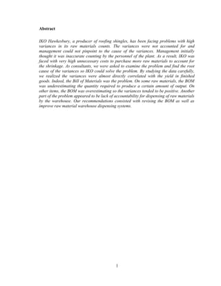
![Background Information
IKO was started in Alberta in 1951, and originally produced asphalt saturated kraft
paper. IKO branched out into a variety of roofing products, and now primarily
manufactures shingles. Through acquisition and building new factories, IKO has become
a global company with manufacturing plants and sales offices in Canada, the Unites
States, Europe, and China. The manufacturing plant in Hawkesbury, Ontario, known as
IKO Hawkesbury, is the facility where this project is based. [1]
A vertically integrated company, IKO even mines its own mineral granules. It has
become the global leader of waterproofing materials for both manufacturing and supply,
and is also the largest exporter of asphalt shingles in the world. The manufacturing plant
located in Brampton, Ontario is responsible for quality control for all locations, and also
reviews, monitors, and improves production processes. The research conducted at this
facility is the basis for the production targets and waste expectations given to individual
manufacturing plants. [1]
The IKO Hawkesbury manufacturing facility has an expected raw materials
efficiency of 98%. According to head office policy, a raw materials inventory count
should be conducted monthly. IKO Hawkesbury has recently implemented a new system
that includes a weekly count of almost all raw materials, as a result of larger than
expected monthly variances. An employee completes the count and compares the figures
calculated to the expected quantity of raw material in stock. There is not currently a
specific procedure in place to determine whether a recount is required, and thus it is at the
employees’ discretion to decide whether the actual values are acceptable in comparison to
the expected value. [Appendix 4:1]
Production at IKO Hawkesbury is constant, and, as a result, little waste occurs. An
exception to this is when the machines need to be reset to accommodate a different size
or colour of shingle, in which case the remainder of the raw materials on the line are
disposed of. It is the belief of plant manager Michael Horner that human error is the
primary cause of the raw materials variance. One of the largest concerns for IKO
Hawkesbury is the variance for asphalt, as it is one of the highest-cost raw materials.
2](data:image/gif;base64,R0lGODlhAQABAIAAAAAAAP///yH5BAEAAAAALAAAAAABAAEAAAIBRAA7)