4. 1 Introduction
1.1 What is cvx?
cvx is a modeling system for disciplined convex programming. Disciplined convex pro-
grams, or DCPs, are convex optimization problems that are described using a limited
set of construction rules, which enables them to be analyzed and solved efficiently.
cvx can solve standard problems such as linear programs (LPs), quadratic programs
(QPs), second-order cone programs (SOCPs), and semidefinite programs (SDPs);
but compared to directly using a solver for one or these types of problems, cvx can
greatly simplify the task of specifying the problem. cvx can also solve much more
complex convex optimization problems, including many involving nondifferentiable
functions, such as 1 norms. You can use cvx to conveniently formulate and solve
constrained norm minimization, entropy maximization, determinant maximization,
and many other problems.
To use cvx effectively, you need to know at least a bit about convex optimiza-
tion. For background on convex optimization, see the book Convex Optimization
[BV04], available on-line at www.stanford.edu/∼boyd/cvxbook/, or the Stanford
course EE364A, available at www.stanford.edu/class/ee364a/.
cvx is implemented in Matlab [Mat04], effectively turning Matlab into an op-
timization modeling language. Model specifications are constructed using common
Matlab operations and functions, and standard Matlab code can be freely mixed with
these specifications. This combination makes it simple to perform the calculations
needed to form optimization problems, or to process the results obtained from their
solution. For example, it is easy to compute an optimal trade-off curve by forming
and solving a family of optimization problems by varying the constraints. As another
example, cvx can be used as a component of a larger system that uses convex opti-
mization, such as a branch and bound method, or an engineering design framework.
cvx also provides special modes to simplify the construction of problems from two
specific problem classes. In SDP mode, cvx applies a matrix interpretation to the
inequality operator, so that linear matrix inequalities (LMIs) and SDPs may be ex-
pressed in a more natural form. In GP mode, cvx accepts all of the special functions
and combination rules of geometric programming, including monomials, posynomi-
als, and generalized posynomials, and transforms such problems into convex form
so that they can be solved efficiently. For background on geometric programming,
see the tutorial paper [BKVH05], available at www.stanford.edu/∼boyd/papers/
gp tutorial.html.
cvx was designed by Michael Grant and Stephen Boyd, with input from Yinyu Ye;
and was implemented by Michael Grant [GBY06]. It incorporates ideas from earlier
work by L¨fberg [L¨f05], Dahl and Vandenberghe [DV05], Crusius [Cru02], Wu and
o o
Boyd [WB00], and many others. The modeling language follows the spirit of AMPL
[FGK99] or GAMS [BKMR98]; unlike these packages, however, cvx was designed
from the beginning to fully exploit convexity. The specific method for implementing
cvx in Matlab draws heavily from YALMIP [L¨f05]. We also hope to develop versions
o
of cvx for other platforms in the future.
4
5. 1.2 What is disciplined convex programming?
Disciplined convex programming is a methodology for constructing convex optimiza-
tion problems proposed by Michael Grant, Stephen Boyd, and Yinyu Ye [GBY06,
Gra04]. It is meant to support the formulation and construction of optimization
problems that the user intends from the outset to be convex. Disciplined convex
programming imposes a set of conventions or rules, which we call the DCP ruleset.
Problems which adhere to the ruleset can be rapidly and automatically verified as
convex and converted to solvable form. Problems that violate the ruleset are rejected,
even when the problem is convex. That is not to say that such problems cannot be
solved using DCP; they just need to be rewritten in a way that conforms to the DCP
ruleset.
A detailed description of the DCP ruleset is given in §4, and it is important for
anyone who intends to actively use cvx to understand it. The ruleset is simple to
learn, and is drawn from basic principles of convex analysis. In return for accept-
ing the restrictions imposed by the ruleset, we obtain considerable benefits, such as
automatic conversion of problems to solvable form, and full support for nondifferen-
tiable functions. In practice, we have found that disciplined convex programs closely
resemble their natural mathematical forms.
1.3 About this version
Supported solvers. This version of cvx supports two core solvers, SeDuMi [Stu99]
and SDPT3 [TTT06], which is the default. Future versions of cvx may support other
solvers, such as MOSEK [MOS05] or CVXOPT [DV05]. SeDuMi and SDPT3 are
open-source interior-point solvers written in Matlab for LPs, SOCPs, SDPs, and
combinations thereof.
Problems handled exactly. cvx will convert the specified problem to an LP,
SOCP, or SDP, when all the functions in the problem specification can be represented
in these forms. This includes a wide variety of functions, such as minimum and
maximum, absolute value, quadratic forms, the minimum and maximum eigenvalues
of a symmetric matrix, power functions xp , and p norms (both for p rational).
Problems handled with (good) approximations. For a few functions, cvx will
make a (good) approximation to transform the specified problem to one that can
be handled by a combined LP, SOCP, and SDP solver. For example, when a power
function or p -norm is used, with non-rational exponent p, cvx replaces p with a
nearby rational. The log of the normal cumulative distribution log Φ(x) is replaced
with an SDP-compatible approximation.
Problems handled with successive approximation. This version of cvx adds
support for a number of functions that cannot be exactly represented via LP, SOCP, or
SDP, including log, exp, log-sum-exp log(exp x1 +· · ·+exp xn ), entropy, and Kullback-
Leibler divergence. These problems are handled by solving a sequence (typically just
5
6. a handful) of SDPs, which yields the solution to the full accuracy of the core solver.
On the other hand, this technique can be substantially slower than if the core solver
directly handled such functions. The successive approximation method is briefly
described in Appendix D.1. Geometric problems are now solved in this manner as
well; in previous versions, an approximation was made.
Ultimately, we will interface cvx to a solver with native support for such functions,
which result in a large speedup in solving problems with these functions. Until then,
users should be aware that problems involving these functions can be slow to solve
using the current version of cvx. For this reason, when one of these functions is used,
the user will be warned that the successive approximate technique will be used.
We emphasize that most users do not need to know how cvx handles their problem;
what matters is what functions and operations can be handled. For a full list of
functions supported by cvx, see Appendix B, or use the online help function by
typing help cvx/builtins (for functions already in Matlab, such as sqrt or log) or
help cvx/functions (for functions not in Matlab, such as lambda_max).
1.4 Feedback
Please contact Michael Grant (mcgrant@stanford.edu) or Stephen Boyd (boyd@stanford.edu)
with your comments. If you discover what you think is a bug, please include the fol-
lowing in your communication, so we can reproduce and fix the problem:
• the cvx model and supporting data that caused the error
• a copy of any error messages that it produced
• the cvx version number and build number
• the version number of Matlab that you are running
• the name and version of the operating system you are using
The latter three items can all be discovered by typing
cvx_version
at the MATLAB command prompt; simply copy its output into your email message.
1.5 What cvx is not
cvx is not meant to be a tool for checking if your problem is convex. You need
to know a bit about convex optimization to effectively use cvx; otherwise you are
the proverbial monkey at the typewriter, hoping to (accidentally) type in a valid
disciplined convex program.
On the other hand, if cvx accepts your problem, you can be sure it is convex. In
conjunction with a course on (or self study of) convex optimization, cvx (especially,
its error messages) can be very helpful in learning some basic convex analysis. While
6
7. cvx will attempt to give helpful error messages when you violate the DCP ruleset, it
can sometimes give quite obscure error messages.
cvx is not meant for very large problems, so if your problem is very large (for
example, a large image processing problem), cvx is unlikely to work well (or at all).
For such problems you will likely need to directly call a solver, or to develop your
own methods, to get the efficiency you need.
For such problems cvx can play an important role, however. Before starting to
develop a specialized large-scale method, you can use cvx to solve scaled-down or
simplified versions of the problem, to rapidly experiment with exactly what problem
you want to solve. For image reconstruction, for example, you might use cvx to
experiment with different problem formulations on 50 × 50 pixel images.
cvx will solve many medium and large scale problems, provided they have ex-
ploitable structure (such as sparsity), and you avoid for loops, which can be slow in
Matlab, and functions like log and exp that require successive approximation. If you
encounter difficulties in solving large problem instances, please do contact us; we may
be able to suggest an equivalent formulation that cvx can process more efficiently.
7
8. 2 A quick start
Once you have installed cvx (see §A), you can start using it by entering a cvx speci-
fication into a Matlab script or function, or directly from the command prompt. To
delineate cvx specifications from surrounding Matlab code, they are preceded with
the statement cvx_begin and followed with the statement cvx_end. A specification
can include any ordinary Matlab statements, as well as special cvx-specific commands
for declaring primal and dual optimization variables and specifying constraints and
objective functions.
Within a cvx specification, optimization variables have no numerical value; in-
stead, they are special Matlab objects. This enables Matlab to distinguish between
ordinary commands and cvx objective functions and constraints. As Matlab reads
a cvx specification, it builds an internal representation of the optimization problem.
If it encounters a violation of the rules of disciplined convex programming (such as
an invalid use of a composition rule or an invalid constraint), an error message is
generated. When Matlab reaches the cvx_end command, it completes the conversion
of the cvx specification to a canonical form, and calls the underlying core solver to
solve it.
If the optimization is successful, the optimization variables declared in the cvx
specification are converted from objects to ordinary Matlab numerical values that
can be used in any further Matlab calculations. In addition, cvx also assigns a few
other related Matlab variables. One, for example, gives the status of the problem
(i.e., whether an optimal solution was found, or the problem was determined to be
infeasible or unbounded). Another gives the optimal value of the problem. Dual
variables can also be assigned.
This processing flow will become more clear as we introduce a number of simple
examples. We invite the reader to actually follow along with these examples in Mat-
lab, by running the quickstart script found in the examples subdirectory of the cvx
distribution. For example, if you are on Windows, and you have installed the cvx
distribution in the directory D:Matlabcvx, then you would type
cd D:Matlabcvxexamples
quickstart
at the Matlab command prompt. The script will automatically print key excerpts of
its code, and pause periodically so you can examine its output. (Pressing “Enter” or
“Return” resumes progress.) The line numbers accompanying the code excerpts in
this document correspond to the line numbers in the file quickstart.m.
2.1 Least-squares
We first consider the most basic convex optimization problem, least-squares. In a
least-squares problem, we seek x ∈ Rn that minimizes Ax − b 2 , where A ∈ Rm×n
is skinny and full rank (i.e., m ≥ n and Rank(A) = n). Let us create some test
problem data for m, n, A, and b in Matlab:
8
9. 15 m = 16; n = 8;
16 A = randn(m,n);
17 b = randn(m,1);
(We chose small values of m and n to keep the output readable.) Then the least-
squares solution x = (AT A)−1 AT b is easily computed using the backslash operator:
20 x_ls = A b;
Using cvx, the same problem can be solved as follows:
23 cvx_begin
24 variable x(n);
25 minimize( norm(A*x-b) );
26 cvx_end
(The indentation is used for purely stylistic reasons and is optional.) Let us examine
this specification line by line:
• Line 23 creates a placeholder for the new cvx specification, and prepares Matlab
to accept variable declarations, constraints, an objective function, and so forth.
• Line 24 declares x to be an optimization variable of dimension n. cvx requires
that all problem variables be declared before they are used in an objective
function or constraints.
• Line 25 specifies an objective function to be minimized; in this case, the Eu-
clidean or 2 -norm of Ax − b.
• Line 26 signals the end of the cvx specification, and causes the problem to be
solved.
The backslash form is clearly simpler—there is no reason to use cvx to solve a simple
least-squares problem. But this example serves as sort of a “Hello world!” program
in cvx; i.e., the simplest code segment that actually does something useful.
If you were to type x at the Matlab prompt after line 24 but before the cvx_end
command, you would see something like this:
x =
cvx affine expression (8x1 vector)
That is because within a specification, variables have no numeric value; rather, they
are Matlab objects designed to represent problem variables and expressions involving
them. Similarly, because the objective function norm(A*x-b) involves a cvx variable,
it does not have a numeric value either; it is also represented by a Matlab object.
When Matlab reaches the cvx_end command, the least-squares problem is solved,
and the Matlab variable x is overwritten with the solution of the least-squares prob-
lem, i.e., (AT A)−1 AT b. Now x is an ordinary length-n numerical vector, identical to
what would be obtained in the traditional approach, at least to within the accuracy
of the solver. In addition, two additional Matlab variables are created:
9
10. • cvx_optval, which contains the value of the objective function; i.e., Ax − b 2 ;
• cvx_status, which contains a string describing the status of the calculation. In
this case, cvx_status would contain the string Solved. See Appendix C for a
list of the possible values of cvx_status and their meaning.
• cvx_slvtol: the tolerance level achieved by the solver.
• cvx_slvitr: the number of iterations taken by the solver.
All of these quantities, x, cvx_optval, and cvx_status, etc. may now be freely used
in other Matlab statements, just like any other numeric or string values.1
There is not much room for error in specifying a simple least-squares problem,
but if you make one, you will get an error or warning message. For example, if you
replace line 25 with
maximize( norm(A*x-b) );
which asks for the norm to be maximized, you will get an error message stating that
a convex function cannot be maximized (at least in disciplined convex programming):
??? Error using ==> maximize
Disciplined convex programming error:
Objective function in a maximization must be concave.
2.2 Bound-constrained least-squares
Suppose we wish to add some simple upper and lower bounds to the least-squares
problem above: i.e., we wish to solve
minimize Ax − b 2
(1)
subject to l x u,
where l and u are given data, vectors with the same dimension as the variable x. The
vector inequality u v means componentwise, i.e., ui ≤ vi for all i. We can no longer
use the simple backslash notation to solve this problem, but it can be transformed
into a quadratic program (QP), which can be solved without difficulty if you have
some form of QP software available.
Let us provide some numeric values for l and u:
47 bnds = randn(n,2);
48 l = min( bnds, [], 2 );
49 u = max( bnds, [], 2 );
Then if you have the Matlab Optimization Toolbox [Mat05], you can use the quadprog
function to solve the problem as follows:
1
If you type who or whos at the command prompt, you may see other, unfamiliar variables as
well. Any variable that begins with the prefix cvx is reserved for internal use by cvx itself, and
should not be changed.
10
11. 53 x_qp = quadprog( 2*A’*A, -2*A’*b, [], [], [], [], l, u );
This actually minimizes the square of the norm, which is the same as minimizing the
norm itself. In contrast, the cvx specification is given by
59 cvx_begin
60 variable x(n);
61 minimize( norm(A*x-b) );
62 subject to
63 x >= l;
64 x <= u;
65 cvx_end
Three new lines of cvx code have been added to the cvx specification:
• The subject to statement on line 62 does nothing—cvx provides this state-
ment simply to make specifications more readable. It is entirely optional.
• Lines 63 and 64 represent the 2n inequality constraints l x u.
As before, when the cvx_end command is reached, the problem is solved, and the
numerical solution is assigned to the variable x. Incidentally, cvx will not transform
this problem into a QP by squaring the objective; instead, it will transform it into an
SOCP. The result is the same, and the transformation is done automatically.
In this example, as in our first, the cvx specification is longer than the Matlab
alternative. On the other hand, it is easier to read the cvx version and relate it
to the original problem. In contrast, the quadprog version requires us to know in
advance the transformation to QP form, including the calculations such as 2*A’*A
and -2*A’*b. For all but the simplest cases, a cvx specification is simpler, more
readable, and more compact than equivalent Matlab code to solve the same problem.
2.3 Other norms and functions
Now let us consider some alternatives to the least-squares problem. Norm minimiza-
tion problems involving the ∞ or 1 norms can be reformulated as LPs, and solved
using a linear programming solver such as linprog in the Matlab Optimization Tool-
box (see, e.g., [BV04, §6.1]). However, because these norms are part of cvx’s base
library of functions, cvx can handle these problems directly.
For example, to find the value of x that minimizes the Chebyshev norm Ax−b ∞ ,
we can employ the linprog command from the Matlab Optimization Toolbox:
97 f = [ zeros(n,1); 1 ];
98 Ane = [ +A, -ones(m,1) ; ...
99 -A, -ones(m,1) ];
100 bne = [ +b; -b ];
101 xt = linprog(f,Ane,bne);
102 x_cheb = xt(1:n,:);
11
12. With cvx, the same problem is specified as follows:
108 cvx_begin
109 variable x(n);
110 minimize( norm(A*x-b,Inf) );
111 cvx_end
The code based on linprog, and the cvx specification above will both solve the
Chebyshev norm minimization problem, i.e., each will produce an x that minimizes
Ax−b ∞ . Chebyshev norm minimization problems can have multiple optimal points,
however, so the particular x’s produced by the two methods can be different. The
two points, however, must have the same value of Ax − b ∞ .
Similarly, to minimize the 1 norm · 1 , we can use linprog as follows:
139 f = [ zeros(n,1); ones(m,1); ones(m,1) ];
140 Aeq = [ A, -eye(m), +eye(m) ];
141 lb = [ -Inf(n,1); zeros(m,1); zeros(m,1) ];
142 xzz = linprog(f,[],[],Aeq,b,lb,[]);
143 x_l1 = xzz(1:n,:);
The cvx version is, not surprisingly,
149 cvx_begin
150 variable x(n);
151 minimize( norm(A*x-b,1) );
152 cvx_end
cvx automatically transforms both of these problems into LPs, not unlike those gen-
erated manually for linprog.
The advantage that automatic transformation provides is magnified if we consider
functions (and their resulting transformations) that are less well-known than the ∞
and 1 norms. For example, consider the norm
Ax − b lgst,k = |Ax − b|[1] + · · · + |Ax − b|[k] ,
where |Ax − b|[i] denotes the ith largest element of the absolute values of the entries
of Ax − b. This is indeed a norm, albeit a fairly esoteric one. (When k = 1, it
reduces to the ∞ norm; when k = m, the dimension of Ax − b, it reduces to the 1
norm.) The problem of minimizing Ax − b lgst,k over x can be cast as an LP, but
the transformation is by no means obvious so we will omit it here. But this norm is
provided in the base cvx library, and has the name norm_largest, so to specify and
solve the problem using cvx is easy:
179 k = 5;
180 cvx_begin
181 variable x(n);
182 minimize( norm_largest(A*x-b,k) );
183 cvx_end
12
13. Unlike the 1 , 2 , or ∞ norms, this norm is not part of the standard Matlab distri-
bution. Once you have installed cvx, though, the norm is available as an ordinary
Matlab function outside a cvx specification. For example, once the code above is
processed, x is a numerical vector, so we can type
cvx_optval
norm_largest(A*x-b,k)
The first line displays the optimal value as determined by cvx; the second recomputes
the same value from the optimal vector x as determined by cvx.
The list of supported nonlinear functions in cvx goes well beyond norm and
norm_largest. For example, consider the Huber penalty minimization problem
m
minimize i=1 φ((Ax − b)i ),
with variable x ∈ Rn , where φ is the Huber penalty function
|z|2 |z| ≤ 1
φ(z) =
2|z| − 1 |z| ≥ 1.
The Huber penalty function is convex, and has been provided in the cvx function
library. So solving the Huber penalty minimization problem in cvx is simple:
204 cvx_begin
205 variable x(n);
206 minimize( sum(huber(A*x-b)) );
207 cvx_end
cvx automatically transforms this problem into an SOCP, which the core solver then
solves. (The cvx user, however, does not need to know how the transformation is
carried out.)
2.4 Other constraints
We hope that, by now, it is not surprising that adding the simple bounds l x u
to the problems in §2.3 above is as simple as inserting the lines
x >= l;
x <= u;
before the cvx_end statement in each cvx specification. In fact, cvx supports more
complex constraints as well. For example, let us define new matrices C and d in
Matlab as follows,
227 p = 4;
228 C = randn(p,n);
229 d = randn(p,1);
13
14. Now let us add an equality constraint and a nonlinear inequality constraint to the
original least-squares problem:
232 cvx_begin
233 variable x(n);
234 minimize( norm(A*x-b) );
235 subject to
236 C*x == d;
237 norm(x,Inf) <= 1;
238 cvx_end
Both of the added constraints conform to the DCP rules, and so are accepted by cvx.
After the cvx_end command, cvx converts this problem to an SOCP, and solves it.
Expressions using comparison operators (==, >=, etc.) behave quite differently
when they involve cvx optimization variables, or expressions constructed from cvx
optimization variables, than when they involve simple numeric values. For example,
because x is a declared variable, the expression C*x==d in line 236 above causes a
constraint to be included in the cvx specification, and returns no value at all. On the
other hand, outside of a cvx specification, if x has an appropriate numeric value—
for example immediately after the cvx_end command—that same expression would
return a vector of 1s and 0s, corresponding to the truth or falsity of each equality.2
Likewise, within a cvx specification, the statement norm(x,Inf)<=1 adds a nonlinear
constraint to the specification; outside of it, it returns a 1 or a 0 depending on the
numeric value of x (specifically, whether its ∞ -norm is less than or equal to, or more
than, 1).
Because cvx is designed to support convex optimization, it must be able to verify
that problems are convex. To that end, cvx adopts certain construction rules that
govern how constraint and objective expressions are constructed. For example, cvx
requires that the left- and right- hand sides of an equality constraint be affine. So a
constraint such as
norm(x,Inf) == 1;
results in the following error:
??? Error using ==> cvx.eq
Disciplined convex programming error:
Both sides of an equality constraint must be affine.
Inequality constraints of the form f (x) ≤ g(x) or g(x) ≥ f (x) are accepted only if f
can be verified as convex and g verified as concave. So a constraint such as
norm(x,Inf) >= 1;
2
In fact, immediately after the cvx end command above, you would likely find that most if not all
of the values returned would be 0. This is because, as is the case with many numerical algorithms,
solutions are determined only to within some nonzero numeric tolerance. So the equality constraints
will be satisfied closely, but often not exactly.
14
15. results in the following error:
??? Error using ==> cvx.ge
Disciplined convex programming error:
The left-hand side of a ">=" inequality must be concave.
The specifics of the construction rules are discussed in more detail in §4 below. These
rules are relatively intuitive if you know the basics of convex analysis and convex
optimization.
2.5 An optimal trade-off curve
For our final example in this section, let us show how traditional Matlab code and
cvx specifications can be mixed to form and solve multiple optimization problems.
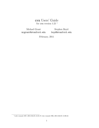
The following code solves the problem of minimizing Ax − b 2 + γ x 1 , for a loga-
rithmically spaced vector of (positive) values of γ. This gives us points on the optimal
trade-off curve between Ax − b 2 and x 1 . An example of this curve is given in
Figure 1.
268 gamma = logspace( -2, 2, 20 );
269 l2norm = zeros(size(gamma));
270 l1norm = zeros(size(gamma));
271 fprintf( 1, ’ gamma norm(x,1) norm(A*x-b)n’ );
272 fprintf( 1, ’---------------------------------------n’ );
273 for k = 1:length(gamma),
274 fprintf( 1, ’%8.4e’, gamma(k) );
275 cvx_begin
276 variable x(n);
277 minimize( norm(A*x-b)+gamma(k)*norm(x,1) );
278 cvx_end
279 l1norm(k) = norm(x,1);
280 l2norm(k) = norm(A*x-b);
281 fprintf( 1, ’ %8.4e %8.4en’, l1norm(k), l2norm(k) );
282 end
283 plot( l1norm, l2norm );
284 xlabel( ’norm(x,1)’ );
285 ylabel( ’norm(A*x-b)’ );
286 grid
Line 277 of this code segment illustrates one of the construction rules to be dis-
cussed in §4 below. A basic principle of convex analysis is that a convex function
can be multiplied by a nonnegative scalar, or added to another convex function, and
the result is then convex. cvx recognizes such combinations and allows them to be
used anywhere a simple convex function can be—such as an objective function to be
minimized, or on the appropriate side of an inequality constraint. So in our example,
the expression
15
16. 3.6
3.4
3.2
3
norm(A*x−b)
2.8
2.6
2.4
2.2
2
0 0.5 1 1.5 2 2.5 3 3.5
norm(x,1)
Figure 1: An example trade-off curve from the quickstart demo, lines 268-286.
norm(A*x-b)+gamma(k)*norm(x,1)
on line 277 is recognized as convex by cvx, as long as gamma(k) is positive or zero. If
gamma(k) were negative, then this expression becomes the sum of a convex term and
a concave term, which causes cvx to generate the following error:
??? Error using ==> cvx.plus
Disciplined convex programming error:
Addition of convex and concave terms is forbidden.
16
17. 3 The basics
3.1 cvx begin and cvx end
All cvx models must be preceded by the command cvx_begin and terminated with
the command cvx_end. All variable declarations, objective functions, and constraints
should fall in between.
The cvx_begin command accepts several modifiers that you may find useful.
For instance, cvx_begin quiet prevents the model from producing any screen out-
put while it is being solved. Additionally, cvx_begin sdp and cvx_begin gp in-
voke special semidefinite and geometric programming modes, discussed in §6 and
§7, respectively. These modifiers may be combined when appropriate; for instance,
cvx_begin sdp quiet invokes SDP mode and silences the solver output.
3.2 Data types for variables
As mentioned above, all variables must be declared using the variable command
(or the variables command; see below) before they can be used in constraints or an
objective function.
Variables can be real or complex; and scalar, vector, matrix, or n-dimensional
arrays. In addition, matrices can have structure as well, such as symmetry or band-
edness. The structure of a variable is given by supplying a list of descriptive keywords
after the name and size of the variable. For example, the code segment
variable w(50) complex;
variable X(20,10);
variable Y(50,50) symmetric;
variable Z(100,100) hermitian toeplitz;
(inside a cvx specification) declares that w is a complex 50-element vector variable, X
is a real 20×10 matrix variable, Y is a real 50×50 symmetric matrix variable, and Z is
a complex 100 × 100 Hermitian Toeplitz matrix variable. The structure keywords can
be applied to n-dimensional arrays as well: each 2-dimensional “slice” of the array is
given the stated structure. The currently supported structure keywords are:
banded(lb,ub) complex diagonal hankel hermitian lower_bidiagonal
lower_hessenberg lower_triangular scaled_identity skew_symmetric
symmetric toeplitz tridiagonal upper_bidiagonal upper_hankel
upper_hessenberg upper_triangular
With a couple of exceptions, the structure keywords are self-explanatory:
• banded(lb,ub): the matrix is banded with a lower bandwidth lb and an upper
bandwidth ub. If both lb and ub are zero, then a diagonal matrix results. ub
can be omitted, in which case it is set equal to lb. For example, banded(1,1)
(or banded(1)) is a tridiagonal matrix.
17
18. • scaled_identity: the matrix is a (variable) multiple of the identity matrix.
This is the same as declaring it to be diagonal and Toeplitz.
• upper_hankel: The matrix is Hankel (i.e., constant along antidiagonals), and
zero below the central antidiagonal, i.e., for i + j > n + 1.
When multiple keywords are supplied, the resulting matrix structure is determined
by intersection; if the keywords conflict, then an error will result.
A variable statement can be used to declare only a single variable, which can
be a bit inconvenient if you have a lot of variables to declare. For this reason, the
variables statement is provided which allows you to declare multiple variables; i.e.,
variables x1 x2 x3 y1(10) y2(10,10,10);
The one limitation of the variables command is that it cannot declare complex or
structured arrays (e.g., symmetric, etc.). These must be declared one at a time, using
the singular variable command.
3.3 Objective functions
Declaring an objective function requires the use of the minimize or maximize func-
tion, as appropriate. (For the benefit of our users with a British influence, the syn-
onyms minimise and maximise are provided as well.) The objective function in a call
to minimize must be convex; the objective function in a call to maximize must be
concave. At most one objective function may be declared in a given cvx specification,
and the objective function must have a scalar value. (For the only exception to this
rule, see the section on defining new functions in §5).
If no objective function is specified, the problem is interpreted as a feasibility
problem, which is the same as performing a minimization with the objective function
set to zero. In this case, cvx_optval is either 0, if a feasible point is found, or +Inf,
if the constraints are not feasible.
3.4 Constraints
The following constraint types are supported in cvx:
• Equality == constraints, where both the left- and right-hand sides are affine
functions of the optimization variables.
• Less-than <=, < inequality constraints, where the left-hand expression is convex,
and the right-hand expression is concave.
• Greater-than >=, > constraints, where the left-hand expression is concave, and
the right-hand expression is convex.
In cvx, the strict inequalities < and > are accepted, but interpreted as the associated
nonstrict inequalities, <= and >=, respectively. We encourage you to use the nonstrict
18
19. forms <= and >=, since they are mathematically correct. (Future versions of cvx
might assign a slightly different meaning to strict inequalities.)
These equality and inequality operators work for arrays. When both sides of
the constraint are arrays of the same size, the constraint is imposed elementwise. For
example, if a and b are m×n matrices, then a<=b is interpreted by cvx as mn (scalar)
inequalities, i.e., each entry of a must be less than or equal to the corresponding entry
of b. cvx also handles cases where one side is a scalar and the other is an array. This
is interpreted as a constraint for each element of the array, with the (same) scalar
appearing on the other side. As an example, if a is an m × n matrix, then a>=0 is
interpreted as mn inequalities: each element of the matrix must be nonnegative.
Note also the important distinction between =, which is an assignment, and ==,
which imposes an equality constraint (inside a cvx specification); for more on this
distinction, see §8.4. Also note that the non-equality operator ~= may not be used in
a constraint; in any case, such constraints are rarely convex. Inequalities cannot be
used if either side is complex.
cvx also supports a set membership constraint; see §3.6.
3.5 Functions
The base cvx function library includes a variety of convex, concave, and affine func-
tions which accept cvx variables or expressions as arguments. Many are common
Matlab functions such as sum, trace, diag, sqrt, max, and min, re-implemented as
needed to support cvx; others are new functions not found in Matlab. A complete
list of the functions in the base library can be found in §B. It’s also possible to add
your own new functions; see §5.
An example of a function in the base library is quad_over_lin, which represents
the quadratic-over-linear function, defined as f (x, y) = xT x/y, with domain Rn ×
R++ , i.e., x is an arbitrary vector in Rn , and y is a positive scalar. (The function also
accepts complex x, but we’ll consider real x to keep things simple.) The quadratic-
over-linear function is convex in x and y, and so can be used as an objective, in an
appropriate constraint, or in a more complicated expression. We can, for example,
minimize the quadratic-over-linear function of (Ax − b, cT x + d) using
minimize( quad_over_lin( A*x-b, c’*x+d ) );
inside a cvx specification, assuming x is a vector optimization variable, A is a matrix,
b and c are vectors, and d is a scalar. cvx recognizes this objective expression as a
convex function, since it is the composition of a convex function (the quadratic-over-
linear function) with an affine function.
You can also use the function quad_over_lin outside a cvx specification. In
this case, it just computes its (numerical) value, given (numerical) arguments. It’s
not quite the same as the expression ((A*x-b)’*(A*x-b))/(c’*x+d), however. This
expression makes sense, and returns a real number, when cT x + d is negative; but
quad_over_lin(A*x-b,c’*x+d) returns +Inf if cT x + d > 0.
19
20. 3.6 Sets
cvx supports the definition and use of convex sets. The base library includes the cone
of positive semidefinite n × n matrices, the second-order or Lorentz cone, and various
norm balls. A complete list of sets supplied in the base library is given in §B.
Unfortunately, the Matlab language does not have a set membership operator,
such as x in S, to denote x ∈ S. So in cvx, we use a slightly different syntax to
require that an expression is in a set. To represent a set we use a function that
returns an unnamed variable that is required to be in the set. Consider, for example,
Sn , the cone of symmetric positive semidefinite n × n matrices. In cvx, we represent
+
this by the function semidefinite(n), which returns an unnamed new variable, that
is constrained to be positive semidefinite. To require that the matrix expression X
be symmetric positive semidefinite, we use the syntax X == semidefinite(n). The
literal meaning of this is that X is constrained to be equal to some unnamed variable,
which is required to be an n × n symmetric positive semidefinite matrix. This is, of
course, equivalent to saying that X must be symmetric positive semidefinite.
As an example, consider the constraint that a (matrix) variable X is a correlation
matrix, i.e., it is symmetric, has unit diagonal elements, and is positive semidefinite.
In cvx we can declare such a variable and impose such constraints using
variable X(n,n) symmetric;
X == semidefinite(n);
diag(X) == ones(n,1);
The second line here imposes the constraint that X be positive semidefinite. (You can
read ‘==’ here as ‘is’, so the second line can be read as ‘X is positive semidefinite’.)
The lefthand side of the third line is a vector containing the diagonal elements of X,
whose elements we require to be equal to one. Incidentally, cvx allows us to simplify
the third line to
diag(X) == 1;
because cvx follows the Matlab convention of handling array/scalar comparisons by
comparing each element of the array independently with the scalar.
If this use of equality constraints to represent set membership remains confusing
or simply aesthetically displeasing, we have create a “pseudo-operator” <In> that
you can use in its place. So, for example, the semidefinite constraint above can be
replaced by
X <In> semidefinite(n);
This is exactly equivalent to using the equality constraint operator, but if you find it
more pleasing, feel free to use it. Implementing this operator required some Matlab
trickery, so don’t expect to be able to use it outside of cvx models.
Sets can be combined in affine expressions, and we can constrain an affine expres-
sion to be in a convex set. For example, we can impose constraints of the form
A*X*A’-X == B*semidefinite(n)*B’;
20
21. where X is an n × n symmetric variable matrix, and A and B are n × n constant
matrices. This constraint requires that AXAT − X = BY B T , for some Y ∈ Sn .+
cvx also supports sets whose elements are ordered lists of quantities. As an ex-
ample, consider the second-order or Lorentz cone,
Qm = { (x, y) ∈ Rm × R | x 2 ≤ y } = epi · 2, (2)
where epi denotes the epigraph of a function. An element of Qm is an ordered list,
with two elements: the first is an m-vector, and the second is a scalar. We can use this
cone to express the simple least-squares problem from §2.1 (in a fairly complicated
way) as follows:
minimize y
(3)
subject to (Ax − b, y) ∈ Qm .
cvx uses Matlab’s cell array facility to mimic this notation:
cvx_begin
variables x(n) y;
minimize( y );
subject to
{ A*x-b, y } <In> lorentz(m);
cvx_end
The function call lorentz(m) returns an unnamed variable (i.e., a pair consisting of
a vector and a scalar variable), constrained to lie in the Lorentz cone of length m. So
the constraint in this specification requires that the pair { A*x-b, y } lies in the
appropriately-sized Lorentz cone.
3.7 Dual variables
When a disciplined convex program is solved, the associated dual problem is also
solved. (In this context, the original problem is called the primal problem.) The
optimal dual variables, each of which is associated with a constraint in the original
problem, give valuable information about the original problem, such as the sensitiv-
ities with respect to perturbing the constraints [BV04, Ch.5]. To get access to the
optimal dual variables in cvx, you simply declare them, and associate them with the
constraints. Consider, for example, the LP
minimize cT x
subject to Ax b,
with variable x ∈ Rn , and m inequality constraints. The dual of this problem is
maximize −bT y
subject to c + AT y = 0
y 0,
where the dual variable y is associated with the inequality constraint Ax b in the
original LP. To represent the primal problem and this dual variable in cvx, we use
the following syntax:
21
22. n = size(A,2);
cvx_begin
variable x(n);
dual variable y;
minimize( c’ * x );
subject to
y : A * x <= b;
cvx_end
The line
dual variable y
tells cvx that y will represent the dual variable, and the line
y : A * x <= b;
associates it with the inequality constraint. Notice how the colon : operator is being
used in a different manner than in standard Matlab, where it is used to construct
numeric sequences like 1:10. This new behavior is in effect only when a dual variable
is present, so there should be no confusion or conflict. No dimensions are given for
y; they are automatically determined from the constraint with which it is associated.
For example, if m = 20, typing y at the Matlab command prompt immediately before
cvx_end yields
y =
cvx dual variable (20x1 vector)
It is not necessary to place the dual variable on the left side of the constraint; for
example, the line above can also be written in this way:
A * x <= b : y;
In addition, dual variables for inequality constraints will always be nonnegative, which
means that the sense of the inequality can be reversed without changing the dual
variable’s value; i.e.,
b >= A * x : y;
yields an identical result. For equality constraints, on the other hand, swapping the
left- and right- hand sides of an equality constraint will negate the optimal value of
the dual variable.
After the cvx_end statement is processed, and assuming the optimization was
successful, cvx assigns numerical values to x and y—the optimal primal and dual
variable values, respectively. Optimal primal and dual variables for this LP must
satisfy the complementary slackness conditions
yi (b − Ax)i = 0, i = 1, . . . , m. (4)
You can check this in Matlab with the line
22
23. y .* (b-A*x)
which prints out the products of the entries of y and b-A*x, which should be nearly
zero. This line must be executed after the cvx_end command (which assigns nu-
merical values to x and y); it will generate an error if it is executed inside the cvx
specification, where y and b-A*x are still just abstract expressions.
If the optimization is not successful, because either the problem is infeasible or
unbounded, then x and y will have different values. In the unbounded case, x will
contain an unbounded direction; i.e., a point x satisfying
cT x = −1, Ax 0, (5)
and y will be filled with NaN values, reflecting the fact that the dual problem is
infeasible. In the infeasible case, x is filled with NaN values, while y contains an
unbounded dual direction; i.e., a point y satisfying
bT y = −1, AT y = 0, y 0 (6)
Of course, the precise interpretation of primal and dual points and/or directions
depends on the structure of the problem. See references such as [BV04] for more on
the interpretation of dual information.
cvx also supports the declaration of indexed dual variables. These prove useful
when the number of constraints in a model (and, therefore, the number of dual
variables) depends upon the parameters themselves. For more information on indexed
dual variables, see §8.5.
3.8 Expression holders
Sometimes it is useful to store a cvx expression into a Matlab variable for future use.
For instance, consider the following cvx script:
variables x y
z = 2 * x - y;
square( z ) <= 3;
quad_over_lin( x, z ) <= 1;
The construction z = 2 * x - y is not an equality constraint; it is an assignment.
It is storing an intermediate calculation 2 * x - y, which is an affine expression,
which is then used later in two different constraints. We call z an expression holder
to differentiate it from a formally declared cvx variable. For more on the critical
differences between assignment and equality, see Section §8.4.
Often it will be useful to accumulate an array of expressions into a single Matlab
variable. Unfortunately, a somewhat technical detail of the Matlab object model can
cause problems in such cases. Consider this construction:
variable u(9);
x(1) = 1;
23
24. for k = 1 : 9,
x(k+1) = sqrt( x(k) + u(k) );
end
This seems reasonable enough: x should be a vector whose first value is 1, and whose
subsequent values are concave cvx expressions. But if you try this in a cvx model,
Matlab will give you a rather cryptic error:
??? The following error occurred converting from cvx to double:
Error using ==> double
Conversion to double from cvx is not possible.
The reason this occurs is that the Matlab variable x is initialized as a numeric array
when the assignment x(1)=1 is made; and Matlab will not permit cvx objects to be
subsequently inserted into numeric arrays.
The solution is to explicitly declare x to be an expression holder before assigning
values to it. We have provided keywords expression and expressions for just this
purpose, for declaring a single or multiple expression holders for future assignment.
Once an expression holder has been declared, you may freely insert both numeric
and cvx expressions into it. For example, the previous example can be corrected as
follows:
variable u(9);
expression x(10);
x(1) = 1;
for k = 1 : 9,
x(k+1) = sqrt( x(k) + u(k) );
end
cvx will accept this construction without error. You can then use the concave ex-
pressions x(1), . . . , x(10) in any appropriate ways; for example, you could maximize
x(10).
The differences between a variable object and an expression object are quite
significant. A variable object holds an optimization variable, and cannot be over-
written or assigned in the cvx specification. (After solving the problem, however, cvx
will overwrite optimization variables with optimal values.) An expression object, on
the other hand, is initialized to zero, and should be thought of as a temporary place
to store cvx expressions; it can be assigned to, freely re-assigned, and overwritten in
a cvx specification.
Of course, as our first example shows, it is not always necessary to declare an
expression holder before it is created or used. But doing so provides an extra measure
of clarity to models, so we strongly recommend it.
24
25. 4 The DCP ruleset
cvx enforces the conventions dictated by the disciplined convex programming ruleset,
or DCP ruleset for short. cvx will issue an error message whenever it encounters
a violation of any of the rules, so it is important to understand them before begin-
ning to build models. The rules are drawn from basic principles of convex analysis,
and are easy to learn, once you’ve had an exposure to convex analysis and convex
optimization.
The DCP ruleset is a set of sufficient, but not necessary, conditions for convexity.
So it is possible to construct expressions that violate the ruleset but are in fact
convex. As an example consider the entropy function, − n xi log xi , defined for
i=1
x > 0, which is concave. If it is expressed as
- sum( x .* log( x ) )
cvx will reject it, because its concavity does not follow from any of the composition
rules. (Specifically, it violates the no-product rule described in §4.4.) Problems
involving entropy, however, can be solved, by explicitly using the entropy function,
sum(entr( x ))
which is in the base cvx library, and thus recognized as concave by cvx. If a convex
(or concave) function is not recognized as convex or concave by cvx, it can be added
as a new atom; see §5. √
As another example consider the function x2 + 1 = [x 1] 2 , which is convex. If
it is written as
norm([x 1])
(assuming x is a scalar variable or affine expression) it will be recognized by cvx
as a convex expression, and therefore can be used in (appropriate) constraints and
objectives. But if it is written as
sqrt(x^2+1)
cvx will reject it, since convexity of this function does not follow from the cvx ruleset.
4.1 A taxonomy of curvature
In disciplined convex programming, a scalar expression is classified by its curvature.
There are four categories of curvature: constant, affine, convex, and concave. For a
function f : Rn → R defined on all Rn , the categories have the following meanings:
constant: f (αx + (1 − α)y) = f (x) ∀x, y ∈ Rn , α ∈ R
affine: f (αx + (1 − α)y) = αf (x) + (1 − α)f (y) ∀x, y ∈ Rn , α ∈ R
convex: f (αx + (1 − α)y) ≤ αf (x) + (1 − α)f (y) ∀x, y ∈ Rn , α ∈ [0, 1]
concave: f (αx + (1 − α)y) ≥ αf (x) + (1 − α)f (y) ∀x, y ∈ Rn , α ∈ [0, 1]
25
26. Of course, there is significant overlap in these categories. For example, constant
expressions are also affine, and (real) affine expressions are both convex and concave.
Convex and concave expressions are real by definition. Complex constant and
affine expressions can be constructed, but their usage is more limited; for example,
they cannot appear as the left- or right-hand side of an inequality constraint.
4.2 Top-level rules
cvx supports three different types of disciplined convex programs:
• A minimization problem, consisting of a convex objective function and zero or
more constraints.
• A maximization problem, consisting of a concave objective function and zero or
more constraints.
• A feasibility problem, consisting of one or more constraints.
4.3 Constraints
Three types of constraints may be specified in disciplined convex programs:
• An equality constraint, constructed using ==, where both sides are affine.
• A less-than inequality constraint, using either <= or <, where the left side is
convex and the right side is concave.
• A greater-than inequality constraint, using either >= or >, where the left side is
concave and the right side is convex.
Non-equality constraints, constructed using ~=, are never allowed. (Such constraints
are not convex.)
One or both sides of an equality constraint may be complex; inequality constraints,
on the other hand, must be real. A complex equality constraint is equivalent to two
real equality constraints, one for the real part and one for the imaginary part. An
equality constraint with a real side and a complex side has the effect of constraining
the imaginary part of the complex side to be zero.
As discussed in §3.6 above, cvx enforces set membership constraints (e.g., x ∈ S)
using equality constraints. The rule that both sides of an equality constraint must
be affine applies to set membership constraints as well. In fact, the returned value of
set atoms like semidefinite() and lorentz() is affine, so it is sufficient to simply
verify the remaining portion of the set membership constraint. For composite values
like { x, y }, each element must be affine.
In this version, strict inequalities <, > are interpreted identically to nonstrict
inequalities >=, <=. Eventually cvx will flag strict inequalities so that they can be
verified after the optimization is carried out.
26
27. 4.4 Expression rules
So far, the rules as stated are not particularly restrictive, in that all convex programs
(disciplined or otherwise) typically adhere to them. What distinguishes disciplined
convex programming from more general convex programming are the rules governing
the construction of the expressions used in objective functions and constraints.
Disciplined convex programming determines the curvature of scalar expressions
by recursively applying the following rules. While this list may seem long, it is for
the most part an enumeration of basic rules of convex analysis for combining convex,
concave, and affine forms: sums, multiplication by scalars, and so forth.
• A valid constant expression is
– any well-formed Matlab expression that evaluates to a finite value.
• A valid affine expression is
– a valid constant expression;
– a declared variable;
– a valid call to a function in the atom library with an affine result;
– the sum or difference of affine expressions;
– the product of an affine expression and a constant.
• A valid convex expression is
– a valid constant or affine expression;
– a valid call to a function in the atom library with a convex result;
– an affine scalar raised to a constant power p ≥ 1, p = 3, 5, 7, 9, ...;
– a convex scalar quadratic form (§4.8);
– the sum of two or more convex expressions;
– the difference between a convex expression and a concave expression;
– the product of a convex expression and a nonnegative constant;
– the product of a concave expression and a nonpositive constant;
– the negation of a concave expression.
• A valid concave expression is
– a valid constant or affine expression;
– a valid call to a function in the atom library with a concave result;
– a concave scalar raised to a power p ∈ (0, 1);
– a concave scalar quadratic form (§4.8);
– the sum of two or more concave expressions;
27
28. – the difference between a concave expression and a convex expression;
– the product of a concave expression and a nonnegative constant;
– the product of a convex expression and a nonpositive constant;
– the negation of a convex expression.
If an expression cannot be categorized by this ruleset, it is rejected by cvx. For matrix
and array expressions, these rules are applied on an elementwise basis. We note that
the set of rules listed above is redundant; there are much smaller, equivalent sets of
rules.
Of particular note is that these expression rules generally forbid products between
nonconstant expressions, with the exception of scalar quadratic forms (see §4.8 below).
For example, the expression x*sqrt(x) happens to be a convex function of x, but
its convexity cannot be verified using the cvx ruleset, and so is rejected. (It can be
expressed as x^(3/2) or pow_p(x,3/2), however.) We call this the no-product rule,
and paying close attention to it will go a long way to insuring that the expressions
you construct are valid.
4.5 Functions
In cvx, functions are categorized in two attributes: curvature (constant, affine, con-
vex, or concave) and monotonicity (nondecreasing, nonincreasing, or nonmonotonic).
Curvature determines the conditions under which they can appear in expressions ac-
cording to the expression rules given in §4.4 above. Monotonicity determines how
they can be used in function compositions, as we shall see in §4.6 below.
For functions with only one argument, the categorization is straightforward. Some
examples are given in the table below.
Function Meaning Curvature Monotonicity
sum( x ) i xi affine nondecreasing
abs( x ) |x|
√ convex nonmonotonic
sqrt( x ) x concave nondecreasing
Following standard practice in convex analysis, convex functions are interpreted
as +∞ when the argument is outside the domain of the function, and concave func-
tions are interpreted as −∞ when the argument is outside its domain. In other
words, convex and concave functions in cvx are interpreted as their extended-valued
extensions.
This has the effect of automatically constraining the argument of a function to be
in the function’s domain. For example, if we form sqrt(x+1) in a cvx specification,
where x is a variable, then x will automatically be constrained to be larger than or
equal to −1. There is no need to add a separate constraint, x>=-1, to enforce this.
Monotonicity of a function is determined in the extended sense, i.e., including the
values of the argument outside its domain. For example, sqrt(x) is determined to be
nondecreasing since its value is constant (−∞) for negative values of its argument;
then jumps up to 0 for argument zero, and increases for positive values of its argument.
28
29. cvx does not consider a function to be convex or concave if it is so only over
a portion of its domain, even if the argument is constrained to lie in one of these
portions. As an example, consider the function 1/x. This function is convex for x > 0,
and concave for x < 0. But you can never write 1/x in cvx (unless x is constant),
even if you have imposed a constraint such as x>=1, which restricts x to lie in the
convex portion of function 1/x. You can use the cvx function inv_pos(x), defined
as 1/x for x > 0 and ∞ otherwise, for the convex portion of 1/x; cvx recognizes this
function as convex and nonincreasing. In cvx, you can express the concave portion
of 1/x, where x is negative, using -inv_pos(-x), which will be correctly recognized
as concave and nonincreasing.
For functions with multiple arguments, curvature is always considered jointly, but
monotonicity can be considered on an argument-by-argument basis. For example,
|x|2 /y y>0
quad_over_lin( x, y ) convex, nonincreasing in y
+∞ y≤0
is jointly convex in both arguments, but it is monotonic only in its second argument.
In addition, some functions are convex, concave, or affine only for a subset of its
arguments. For example, the function
norm( x, p ) x p (1 ≤ p) convex in x, nonmonotonic
is convex only in its first argument. Whenever this function is used in a cvx speci-
fication, then, the remaining arguments must be constant, or cvx will issue an error
message. Such arguments correspond to a function’s parameters in mathematical
terminology; e.g.,
fp (x) : Rn → R, fp (x) x p
So it seems fitting that we should refer to such arguments as parameters in this
context as well. Henceforth, whenever we speak of a cvx function as being convex,
concave, or affine, we will assume that its parameters are known and have been given
appropriate, constant values.
4.6 Compositions
A basic rule of convex analysis is that convexity is closed under composition with an
affine mapping. This is part of the DCP ruleset as well:
• A convex, concave, or affine function may accept an affine expression (of compat-
ible size) as an argument. The result is convex, concave, or affine, respectively.
For example, consider the function square( x ), which is provided in the cvx atom
library. This function squares its argument; i.e., it computes x.*x. (For array ar-
guments, it squares each element independently.) It is in the cvx atom library, and
known to be convex, provided its argument is real. So if x is a real variable of
dimension n, a is a constant n-vector, and b is a constant, the expression
square( a’ * x + b )
29
30. is accepted by cvx, which knows that it is convex.
The affine composition rule above is a special case of a more sophisticated compo-
sition rule, which we describe now. We consider a function, of known curvature and
monotonicity, that accepts multiple arguments. For convex functions, the rules are:
• If the function is nondecreasing in an argument, that argument must be convex.
• If the function is nonincreasing in an argument, that argument must be concave.
• If the function is neither nondecreasing or nonincreasing in an argument, that
argument must be affine.
If each argument of the function satisfies these rules, then the expression is accepted
by cvx, and is classified as convex. Recall that a constant or affine expression is
both convex and concave, so any argument can be affine, including as a special case,
constant.
The corresponding rules for a concave function are as follows:
• If the function is nondecreasing in an argument, that argument must be concave.
• If the function is nonincreasing in an argument, that argument must be convex.
• If the function is neither nondecreasing or nonincreasing in an argument, that
argument must be affine.
In this case, the expression is accepted by cvx, and classified as concave.
For more background on these composition rules, see [BV04, §3.2.4]. In fact, with
the exception of scalar quadratic expressions, the entire DCP ruleset can be thought
of as special cases of these six rules.
Let us examine some examples. The maximum function is convex and nonde-
creasing in every argument, so it can accept any convex expressions as arguments.
For example, if x is a vector variable, then
max( abs( x ) )
obeys the first of the six composition rules and is therefore accepted by cvx, and
classified as convex.
As another example, consider the sum function, which is both convex and concave
(since it is affine), and nondecreasing in each argument. Therefore the expressions
sum( square( x ) )
sum( sqrt( x ) )
are recognized as valid in cvx, and classified as convex and concave, respectively. The
first one follows from the first rule for convex functions; and the second one follows
from the first rule for concave functions.
Most people who know basic convex analysis like to think of these examples in
terms of the more specific rules: a maximum of convex functions is convex, and a sum
of convex (concave) functions is convex (concave). But these rules are just special
30
31. cases of the general composition rules above. Some other well known basic rules that
follow from the general composition rules are: a nonnegative multiple of a convex
(concave) function is convex (concave); a nonpositive multiple of a convex (concave)
function is concave (convex).
Now we consider a more complex example in depth. Suppose x is a vector vari-
able, and A, b, and f are constants with appropriate dimensions. cvx recognizes the
expression
sqrt(f’*x) + min(4,1.3-norm(A*x-b))
as concave. Consider the term sqrt(f’*x). cvx recognizes that sqrt is concave and
f’*x is affine, so it concludes that sqrt(f’*x) is concave. Now consider the second
term min(4,1.3-norm(A*x-b)). cvx recognizes that min is concave and nondecreas-
ing, so it can accept concave arguments. cvx recognizes that 1.3-norm(A*x-b) is
concave, since it is the difference of a constant and a convex function. So cvx con-
cludes that the second term is also concave. The whole expression is then recognized
as concave, since it is the sum of two concave functions.
The composition rules are sufficient but not necessary for the classification to be
correct, so some expressions which are in fact convex or concave will fail to satisfy
them, and so will be rejected by cvx. For example, if x is a vector variable, the
expression
sqrt( sum( square( x ) ) )
is rejected by cvx, because there is no rule governing the composition of a concave
nondecreasing function with a convex function. Of course, the workaround is simple
in this case: use norm( x ) instead, since norm is in the atom library and known by
cvx to be convex.
4.7 Monotonicity in nonlinear compositions
Monotonicity is a critical aspect of the rules for nonlinear compositions. This has
some consequences that are not so obvious, as we shall demonstrate here by example.
Consider the expression
square( square( x ) + 1 )
where x is a scalar variable. This expression is in fact convex, since (x2 + 1)2 =
x4 + 2x2 + 1 is convex. But cvx will reject the expression, because the outer square
cannot accept a convex argument. Indeed, the square of a convex function is not, in
general, convex: for example, (x2 − 1)2 = x4 − 2x2 + 1 is not convex.
There are several ways to modify the expression above to comply with the ruleset.
One way is to write it as x^4 + 2*x^2 + 1, which cvx recognizes as convex, since
cvx allows positive even integer powers using the ^ operator. (Note that the same
technique, applied to the function (x2 −1)2 , will fail, since its second term is concave.)
Another approach is to use the alternate outer function square_pos, included in
the cvx library, which represents the function (x+ )2 , where x+ = max{0, x}. Obvi-
ously, square and square_pos coincide when their arguments are nonnegative. But
31
32. square_pos is nondecreasing, so it can accept a convex argument. Thus, the expres-
sion
square_pos( square( x ) + 1 )
is mathematically equivalent to the rejected version above (since the argument to the
outer function is always positive), but it satisfies the DCP ruleset and is therefore
accepted by cvx.
This is the reason several functions in the cvx atom library come in two forms:
the “natural” form, and one that is modified in such a way that it is monotonic, and
can therefore be used in compositions. Other such “monotonic extensions” include
sum_square_pos and quad_pos_over_lin. If you are implementing a new function
yourself, you might wish to consider if a monotonic extension of that function would
also be useful.
4.8 Scalar quadratic forms
In its original form described in [Gra04, GBY06], the DCP ruleset forbids even the
use of simple quadratic expressions such as x * x (assuming x is a scalar variable).
For practical reasons, we have chosen to make an exception to the ruleset to allow for
the recognition of certain specific quadratic forms that map directly to certain convex
quadratic functions (or their concave negatives) in the cvx atom library:
conj( x ) .* x is replaced with square( x )
y’ * y is replaced with sum_square( y )
(A*x-b)’*Q*(Ax-b) is replaced with quad_form( A * x - b, Q )
cvx detects the quadratic expressions such as those on the left above, and determines
whether or not they are convex or concave; and if so, translates them to an equivalent
function call, such as those on the right above.
cvx examines each single product of affine expressions, and each single squaring
of an affine expression, checking for convexity; it will not check, for example, sums
of products of affine expressions. For example, given scalar variables x and y, the
expression
x ^ 2 + 2 * x * y + y ^2
will cause an error in cvx, because the second of the three terms 2 * x * y, is neither
convex nor concave. But the equivalent expressions
( x + y ) ^ 2
( x + y ) * ( x + y )
will be accepted. cvx actually completes the square when it comes across a scalar
quadratic form, so the form need not be symmetric. For example, if z is a vector
variable, a, b are constants, and Q is positive definite, then
( z + a )’ * Q * ( z + b )
32
33. will be recognized as convex. Once a quadratic form has been verified by cvx, it
can be freely used in any way that a normal convex or concave expression can be, as
described in §4.4.
Quadratic forms should actually be used less frequently in disciplined convex pro-
gramming than in a more traditional mathematical programming framework, where
a quadratic form is often a smooth substitute for a nonsmooth form that one truly
wishes to use. In cvx, such substitutions are rarely necessary, because of its support
for nonsmooth functions. For example, the constraint
sum( ( A * x - b ) .^ 2 ) <= 1
is equivalently represented using the Euclidean norm:
norm( A * x - b ) <= 1
With modern solvers, the second form can be represented using a second-order cone
constraint—so the second form may actually be more efficient. So we encourage you to
re-evaluate the use of quadratic forms in your models, in light of the new capabilities
afforded by disciplined convex programming.
33
34. 5 Adding new functions to the cvx atom library
cvx allows new convex and concave functions to be defined and added to the atom
library, in two ways, described in this section. The first method is simple, and can
(and should) be used by many users of cvx, since it requires only a knowledge of the
basic DCP ruleset. The second method is very powerful, but a bit complicated, and
should be considered an advanced technique, to be attempted only by those who are
truly comfortable with convex analysis, disciplined convex programming, and cvx in
its current state.
Please do let us know if you have implemented a convex or concave function that
you think would be useful to other users; we will be happy to incorporate it in a
future release.
5.1 New functions via the DCP ruleset
The simplest way to construct a new function that works within cvx is to construct it
using expressions that fully conform to the DCP ruleset. To illustrate this, consider
the convex deadzone function, defined as
0 |x| ≤ 1
f (x) = max{|x| − 1, 0} = x−1 x>1
−1 − x x < −1
To implement this function in cvx, simply create a file deadzone.m containing
function y = deadzone( x )
y = max( abs( x ) - 1, 0 )
This function works just as you expect it would outside of cvx—i.e., when its argu-
ment is numerical. But thanks to Matlab’s operator overloading capability, it will
also work within cvx if called with an affine argument. cvx will properly conclude
that the function is convex, because all of the operations carried out conform to the
rules of DCP: abs is recognized as a convex function; we can subtract a constant from
it, and we can take the maximum of the result and 0, which yields a convex function.
So we are free to use deadzone anywhere in a cvx specification that we might use
abs, for example, because cvx knows that it is a convex function.
Let us emphasize that when defining a function this way, the expressions you
use must conform to the DCP ruleset, just as they would if they had been inserted
directly into a cvx model. For example, if we replace max with min above; e.g.,
function y = deadzone_bad( x )
y = min( abs( x ) - 1, 0 )
then the modified function fails to meet the DCP ruleset. The function will work
outside of a cvx specification, happily computing the value min{|x| − 1, 0} for a
numerical argument x. But inside a cvx specification, invoked with a nonconstant
argument, it will not work, because it doesn’t follow the DCP composition rules.
34
35. 5.2 New functions via partially specified problems
A more advanced method for defining new functions in cvx relies on the following
basic result of convex analysis. Suppose that S ⊂ Rn × Rm is a convex set and
g : (Rn × Rm ) → (R ∪ +∞) is a convex function. Then
f : Rn → (R ∪ +∞), f (x) inf { g(x, y) | ∃y, (x, y) ∈ S } (7)
is also a convex function. (This rule is sometimes called the partial minimization
rule.) We can think of the convex function f as the optimal value of a family of
convex optimization problems, indexed or parametrized by x,
minimize g(x, y)
subject to (x, y) ∈ S
with optimization variable y.
One special case should be very familiar: if m = 1 and g(x, y) y, then
f (x) inf { y | ∃y, (x, y) ∈ S }
gives the classic epigraph representation of f :
epi f = S + ({0} × R+ ) ,
where 0 ∈ Rn .
In cvx you can define a convex function in this very manner, that is, as the optimal
value of a parameterized family of disciplined convex programs. We call the under-
lying convex program in such cases an incomplete specification—so named because
the parameters (that is, the function inputs) are unknown when the specification is
constructed. The concept of incomplete specifications can at first seem a bit compli-
cated, but it is very powerful mechanism that allows cvx to support a wide variety
of functions.
Let us look at an example to see how this works. Consider the unit-halfwidth
Huber penalty function h(x):
x2 |x| ≤ 1
h : R → R, h(x) (8)
2|x| − 1 |x| ≥ 1.
We can express the Huber function in terms of the following family of convex QPs,
parameterized by x:
minimize 2v + w2
subject to |x| ≤ v + w (9)
w ≤ 1, v ≥ 0
with scalar variables v and w. The optimal value of this simple QP is equal to the
Huber penalty function of x. We note that the objective and constraint functions in
this QP are (jointly) convex in v, w and x.
We can implement the Huber penalty function in cvx as follows:
35
36. function cvx_optval = huber( x )
cvx_begin
variables w v;
minimize( w^2 + 2 * v );
subject to
abs( x ) <= w + v;
w <= 1; v >= 0;
cvx_end
If huber is called with a numeric value of x, then upon reaching the cvx_end state-
ment, cvx will find a complete specification, and solve the problem to compute the
result. cvx places the optimal objective function value into the variable cvx_optval,
and function returns that value as its output. Of course, it’s very inefficient to com-
pute the Huber function of a numeric value x by solving a QP. But it does give the
correct value (up to the core solver accuracy).
What is most important, however, is that if huber is used within a cvx specifica-
tion, with an affine cvx expression for its argument, then cvx will do the right thing.
In particular, cvx will recognize the Huber function, called with affine argument, as
a valid convex expression. In this case, the function huber will contain a special
Matlab object that represents the function call in constraints and objectives. Thus
the function huber can be used anywhere a traditional convex function can be used,
in constraints or objective functions, in accordance with the DCP ruleset.
There is a corresponding development for concave functions as well. Given a
convex set S as above, and a concave function g : (Rn × Rm ) → (R ∪ −∞), the
function
f : R → (R ∪ −∞), f (x) sup { g(x, y) | ∃y, (x, y) ∈ S } (10)
is concave. If g(x, y) y, then
f (x) sup { y | ∃y, (x, y) ∈ S } (11)
gives the hypograph representation of f :
hypo f = S − Rn .
+
In cvx, a concave incomplete specification is simply one that uses a maximize ob-
jective instead of a minimize objective; and if properly constructed, it can be used
anywhere a traditional concave function can be used within a cvx specification.
For an example of a concave incomplete specification, consider the function
f : Rn×n → R, f (X) = λmin (X + X T ) (12)
Its hypograph can be represented using a single linear matrix inequality:
hypo f = { (X, t) | f (X) ≥ t } = (X, t) | X + X T − tI 0 (13)
So we can implement this function in cvx as follows:
36
37. function cvx_optval = lambda_min_symm( X )
n = size( X, 1 );
cvx_begin
variable y;
maximize( y );
subject to
X + X’ - y * eye( n ) == semidefinite( n );
cvx_end
If a numeric value of X is supplied, this function will return min(eig(X+X’)) (to within
numerical tolerances). However, this function can also be used in cvx constraints and
objectives, just like any other concave function in the atom library.
There are two practical issues that arise when defining functions using incomplete
specifications, both of which we will illustrate using our huber example above. First of
all, as written the function works only with scalar values. To apply it (elementwise) to
a vector requires that we iterate through the elements in a for loop—a very inefficient
enterprise, particularly in cvx. A far better approach is to extend the huber function
to handle vector inputs. This is, in fact, rather simple to do: we simply create a
multiobjective version of the problem:
function cvx_optval = huber( x )
sx = size( x );
cvx_begin
variables w( sx ) v( sx );
minimize( w .^ 2 + 2 * v );
subject to
abs( x ) <= w + v;
w <= 1; v >= 0;
cvx_end
This version of huber will in effect create sx “instances” of the problem in parallel;
and when used in a cvx specification, will be handled correctly.
The second issue is that if the input to huber is numeric, then direct computation
is a far more efficient way to compute the result than solving a QP. (What is more,
the multiobjective version cannot be used with numeric inputs.) One solution is to
place both versions in one file, with an appropriate test to select the proper version
to use:
function cvx_optval = huber( x )
if isnumeric( x ),
xa = abs( x );
flag = xa < 1;
cvx_optval = flag .* xa.^2 + (~flag) * (2*xa-1);
else,
sx = size( x );
cvx_begin
37
38. variables w( sx ) v( sx );
minimize( w .^ 2 + 2 * v );
subject to
abs( x ) <= w + v;
w <= 1; v >= 0;
cvx_end
end
Alternatively, you can create two separate versions of the function, one for numeric
input and one for cvx expressions, and place the cvx version in a subdirectory called
@cvx. (Do not include this directory in your Matlab path; only include its parent.)
Matlab will automatically call the version in the @cvx directory when one of the
arguments is a cvx variable. This is the approach taken for the version of huber
found in the cvx atom library.
One good way to learn more about using incomplete specifications is to examine
some of the examples already in the cvx atom library. Good choices include huber,
inv_pos, lambda_min, lambda_max, matrix_frac, quad_over_lin, sum_largest,
and others. Some are a bit difficult to read because of diagnostic or error-checking
code, but these are relatively simple.
38
39. 6 Semidefinite programming using cvx
Those who are familiar with semidefinite programming (SDP) know that the con-
straints that utilize the set semidefinite(n) in §3.6 above are, in practice, typi-
cally expressed using linear matrix inequality (LMI) notation. For example, given
X = X T ∈ Rn×n , the constraint X 0 denotes that X ∈ Sn ; that is, that X is
+
positive semidefinite.
cvx provides a special SDP mode which allows this LMI convention to be employed
inside cvx models using Matlab’s standard inequality operators >=, <=, etc.. In order
to use it, one must simply begin a model with the statement cvx_begin sdp or
cvx_begin SDP instead of simply cvx_begin. When SDP mode is engaged, cvx
interprets certain inequality constraints in a different manner. To be specific:
• Equality constraints are interpreted the same (i.e., elementwise).
• Inequality constraints involving vectors and scalars are interpreted the same;
i.e., elementwise.
• Inequality constraints involving non-square matrices are disallowed ; attempt-
ing to use them causes an error. If you wish to do true elementwise com-
parison of matrices X and Y, use a vectorization operation X(:) <= Y(:) or
vec( X ) <= vec( Y ). (vec is a function provided by cvx that is equivalent
to the colon operation.)
• Inequality constraints involving real, square matrices are interpreted as follows:
X >= Y and X > Y become X - Y == semidefinite(n)
X <= Y and X < Y become Y - X == semidefinite(n)
If either side is complex, then the inequalities are interpreted as follows:
X >= Y and X > Y become X - Y == hermitian_semidefinite(n)
X <= Y and X < Y become Y - X == hermitian_semidefinite(n)
In the above, n=max(size(X,1),size(Y,1)).
• There is one additional restriction: both X and Y must be the same size, or one
must be the scalar zero. For example, if X and Y are matrices of size n,
X >= 1 or 1 >= Y illegal
X >= ones(n,n) or ones(n,n) >= Y legal
X >= 0 or 0 >= Y legal
In effect, cvx enforces a stricter interpretation of the inequality operators for
LMI constraints.
39
40. • Note that LMI constraints enforce symmetry (real or Hermitian, as appropriate)
on their inputs. Unlike SDPSOL [WB00], cvx does not extract the symmetric
part for you: you must take care to insure symmetry yourself. Since cvx sup-
ports the declaration of symmetric matrices, this is reasonably straightforward.
If cvx cannot determine that an LMI is symmetric, a warning will be issued.
• A dual variable, if supplied, will be applied to the converted equality constraint.
It will be given a positive semidefinite value if an optimal point is found.
So, for example, the cvx model found in the file examples/closest_toeplitz_sdp.m,
cvx_begin
variable Z(n,n) hermitian toeplitz
dual variable Q
minimize( norm( Z - P, ’fro’ ) )
Z == hermitian_semidefinite( n ) : Q;
cvx_end
can also be written as follows:
cvx_begin sdp
variable Z(n,n) hermitian toeplitz
dual variable Q
minimize( norm( Z - P, ’fro’ ) )
Z >= 0 : Q;
cvx_end
Many other examples in the cvx example library utilize semidefinite constraints; and
all of them use SDP mode. To find them, simply search for the text cvx_begin sdp
in the examples/ subdirectory tree using your favorite file search tool. One of these
examples is reproduced in §8.5.
Since semidefinite programming is popular, some may wonder why SDP mode is
not the default behavior. The reason for this is that we place a strong emphasis
on maintaining consistency between Matlab’s native behavior and that of cvx; and
the use of the >=, <=, >, < operators to create LMIs represents a deviation from
that ideal. For example, the expression Z >= 0 in the example above constrains
the variable Z to be positive semidefinite. But after the model has been solved and
Z has been replaced with a numeric value, the expression Z >= 0 will test for the
elementwise nonnegativity of Z. To verify that the numeric value of Z is, in fact,
positive semidefinite, you must perform a test like min(eig(Z)) >= 0.
40
41. 7 Geometric programming using cvx
Geometric programs (GPs) are special mathematical programs that can be converted
to convex form using a change of variables. The convex form of GPs can be expressed
as DCPs, but cvx also provides a special mode that allows a GP to be specified in
its native form. cvx will automatically perform the necessary conversion, compute
a numerical solution, and translate the results back to the original problem. For a
tutorial on geometric programming, we refer the reader to [BKVH05].
To utilize GP mode, you must begin your cvx specification with the command
cvx_begin gp or cvx_begin GP instead of simply cvx_begin. For example, the
following code, found in the example library at gp/max_volume_box.m, determines
the maximum volume box subject to various area and ratio constraints:
cvx_begin gp
variables w h d
maximize( w * h * d )
subject to
2*(h*w+h*d) <= Awall;
w*d <= Afloor;
h/w >= alpha;
h/w <= beta;
d/w >= gamma;
d/w <= delta;
cvx_end
As the example illustrates, cvx supports the construction of monomials and posyn-
omials using addition, multiplication, division (when appropriate), and powers. In
addition, cvx supports the construction of generalized geometric programs (GGPs),
by permitting the use of generalized posynomials wherever posynomials are permitted
in standard GP [BKVH05].
The solvers used in this version of cvx do not support geometric programming
natively. Instead, they are solved using the successive approximation technique de-
scribed in Appendix D.1. This means that solving GPs can be slow, but for small
and medium sized problems, the method works well.
In the remainder of this section, we will describe specific rules that apply when
constructing models in GP mode.
7.1 Top-level rules
cvx supports three types of geometric programs:
• A minimization problem, consisting of a generalized posynomial objective and
zero or more constraints.
• A maximization problem, consisting of a monomial objective and zero or more
constraints.
41
42. • A feasibility problem, consisting of one or more constraints.
The asymmetry between minimizations and maximizations—specifically, that only
monomial objectives are allowed in the latter—is an unavoidable artifact of the ge-
ometry of GPs and GGPs.
7.2 Constraints
Three types of constraints may be specified in geometric programs:
• An equality constraint, constructed using ==, where both sides are monomials.
• A less-than inequality constraint <=, < where the left side is a generalized posyn-
omial and the right side is a monomial.
• A greater-than inequality constraint >=, > where the left side is a monomial and
the right side is a generalized posynomial.
As with DCPs, non-equality constraints are not permitted.
7.3 Expressions
The basic building blocks of generalized geometric programming are monomials,
posynomials, and generalized posynomials. A valid monomial is
• a declared variable;
• the product of two or more monomials;
• the ratio of two monomials;
• a monomial raised to a real power; or
• a call to one of the following functions with monomial arguments: prod, cumprod,
geo_mean, sqrt.
A valid posynomial expression is
• a valid monomial;
• the sum of two or more posynomials;
• the product of two or more posynomials;
• the ratio of a posynomial and a monomial;
• a posynomial raised to a positive integral power; or
• a call to one of the following functions with posynomial arguments: sum, cumsum,
mean, prod, cumprod.
42