2. Introduction
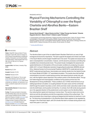
The Royal-Charlotte Bank (RCB) and the Abrolhos Bank (AB) are localized between 17°20’-
18°10’S and 38°35’-39°20’W (Fig. 1) and comprise an extension of the Eastern Brazilian Conti-
nental Shelf (EBS) [1]. This section of the EBS is characterized by a wide continental shelf that
extends almost 200 km in front of Caravelas (BA), as shown in Fig. 1. This region is an excep-
tion in an otherwise regular and narrow shelf. The northern part of the AB provides a home to
the largest and richest reef system in the South Atlantic (Abrolhos reef system), which differs
from the Caribbean reef system with respect to its reef morphology, reef building fauna and de-
positional setting [2]. The Abrolhos Shelf also harbors the largest continuous rhodolith bed in
the world [3], which thrives in the outer and deeper parts of the Bank; the main reef-building
corals, in contrast, are primarily restricted to the shallow areas (30–70 m depths).
Although phytoplankton biomass and turbidity have been frequently used as indicators of
water quality in coral reef systems (e.g., [4]), there is little information on the seasonal and spa-
tial distributions of chlorophyll-a (Chl-a) in the AB and RCB. The few existing oceanographic
studies (e.g., [5], [6]) characterized this region as a transition zone between the low-productivi-
ty area found to the north [7] and the southern area in which coastal, shelf edge, and eddy-in-
duced upwelling enhance the local productivity [8]. Mean Chl-a values of 1.22 mg m-3
(at the
surface) and 0.86 mg m-3
(at the bottom) were reported by [9] for the inner reefs of Coroa
Fig 1. The study area showing the location of the five stations (PT1 to PT5) analyzed. Additionally, three cross-shore transects (R1—blue, R2—yellow
and R4—green) and one alongshore transect (R3—cyan) were used to evaluate the seasonal variation of temperature in the water column throughout the
study area. In situ wind data were obtained from a PIRATA buoy (PB in the left figure) and in situ current information was collected from a deployment
designated by CD (figure on the right). RF stands for the Recife de Fora (Outer Reef). The isobaths shown are 25, 50, 200, 500, 1000 and 2000 m.
doi:10.1371/journal.pone.0117082.g001
Physical Forcing Mechanisms and Chlorophyll-a over the Abrolhos Bank
PLOS ONE | DOI:10.1371/journal.pone.0117082 February 20, 2015 2 / 21
data collection and analysis, decision to publish, or
preparation of the manuscript.
Competing Interests: The co-author Fabiano Lopes
Thompson is a PLOS ONE Editorial Board member.
This does not alter the authors' adherence to PLOS
ONE Editorial policies and criteria.
3. Vermelha and Ponta Grande (just north and inshore of Recife de Fora—RF in Fig. 1). In con-
trast, the Chl-a concentration was approximately one third lower in both surface and bottom
waters for the offshore reef of Recife de Fora (Fig. 1). Differences in Chl-a between nearshore
and offshore reefs reflect the influence from terrestrial and nearshore sources of nutrients [9].
Due to the low riverine discharge, the most direct effects of land runoff are confined to the
coastal area [10]. These effects present a significant seasonal variation in parameters such as
nutrients and suspended material [11]. Under the influence of a tropical humid climate, the
freshwater runoff is highest during the summer-wet season (December-April). Sediment resus-
pension forced by wind stress, primarily during winter storms, also affects the coastal reefs
[12]. The Brazil Current (BC), which flows from lower to higher latitudes along the upper con-
tinental slope, intrudes over the AB, renewing it with clear and oligotrophic oceanic waters. Ac-
cording to [2], this process helps mitigate the land impacts on offshore reefs. To a lesser extent,
wind-driven and tidal currents also contribute to inducing oligotrophic conditions over the AB
[13].
Studies (e.g., [14], [15]) have reported that the coral reefs in the AB have been impacted by
coastal eutrophication associated with sewage pollution. This problem, which is associated
with the growing pressure of economic activities that have high potential for environmental
impact (e.g., fishing, mining, oil and gas exploitation and dredging), has created a demand for
conservation and for broader management strategies of AB marine resources [16]. However, to
implement any conservation plan or management strategy, it is first necessary to improve the
understanding of the oceanographic and land-driven influences on the AB and
RCB ecosystem.
Changes in phytoplankton biomass and productivity at seasonal to inter-annual time scales
are very important components of the total variability associated with ocean biological and bio-
geochemical processes [17]. Furthermore, understanding the spatial and temporal patterns in
phytoplankton distribution can provide important information about fluctuations in coral reef
health [18]. Though a significant understanding of the circulation of the AB was developed
using ocean models over the last decade, we still know little about how that circulation relates
to biological processes in the water column. This lack of information is primarily due to the
lack of comprehensive observational data. Most of the available oceanographic and biological
data are restricted in both space and time and are thus not suitable to study patterns over the
AB and RCB.
Few studies have explicitly investigated the relationship between the meteorological and
oceanographic conditions and the phytoplankton dynamics. Most such studies have associated
the wintertime increase in Chl-a concentration with the wind regime and associated turbulence
(e.g., [19], [20]). However, other factors controlling mixed layer dynamics such as heat fluxes
have not been considered. In this study, a combination of satellite-derived Chl-a data and nu-
merical simulation results was analyzed to investigate the patterns and mechanisms behind
phytoplankton variability in the AB and RCB regions. From these data, a better understanding
of the link between changes in meteorological and oceanographic parameters and phytoplank-
ton dynamics can be reached. This article is organized as follows: the data and methods are pre-
sented in section 2, and the results are described in section 3. A discussion of the results is
presented in Section 4, and the conclusions are drawn in the final section.
Data and Methods
Time series of satellite-derived Chl-a were constructed for five locations (one over the RCB and
four over the AB—Fig. 1) from nine years (2003 to 2011) of 8-day composite Chl-a imagery ac-
quired from MODIS level 3 products (freely available from oceancolor.gsfc.nasa.gov). Their
Physical Forcing Mechanisms and Chlorophyll-a over the Abrolhos Bank
PLOS ONE | DOI:10.1371/journal.pone.0117082 February 20, 2015 3 / 21
4. locations were chosen based not only on the spatial representativeness of the study area but
also on the spatial-temporal variability observed in the mean seasonal Chl-a images. Points
PT1 and PT3 are located where the benthos is covered by coral reefs, and points PT2, PT4 and
PT5 are located in rhodolith-covered benthic regions [16]. Missing data were filled in using a
mean climatological value for the same point and represented less than 30% of the dataset for
each location.
Bio-optical and atmospheric correction algorithms are important components in processing
satellite ocean color data. Most bio-optical algorithms have been empirically derived ([21], [22])
and quantify the Chl-a concentration as a function of the blue-to-green reflectance ratio [23].
These algorithms perform well in Case 1 waters but exhibit limitations in optically complex wa-
ters in which optically active components other than chlorophyll are present. The comparison
between in situ and satellite-derived Chl-a has been used to ensure that satellite-derived measure-
ments are representative of the true Chl-a concentrations; several studies have evaluated the per-
formance of the standard MODIS algorithms for locations worldwide (e.g., [24], [25], [26]).
However, there are no validation studies of MODIS-derived Chl-a concentration in the area of
the present study, so the data presented here should be considered primarily in terms of their
variability rather than their absolute values. Nevertheless, the in situ Chl-a results reported by
[27] for January 2009 and 2010 for the AB (0.17 to 0.50 mg m-3
) were in the range of those found
in this study.
To investigate and quantify the phenology of the seasonal bloom in tropical latitudes, the
8-day Chl-a values were averaged monthly over the 9-year period and fitted to a Gaussian func-
tion [28] of Chl-a versus time according to the methodology described in [29], [30], [31] as
ChlðtÞ ¼ Chlo þ
h
s
ffiffiffiffiffiffi
2p
p exp À
ðt À tmaxÞ
2
2s2
Equation1
where Chlo is the baseline of Chl-a concentration (mg m-3
), tmax (month) is the time at the
peak concentration and σ (month) is the standard deviation of the Gaussian curve. The peak
concentration is defined by (h=s
ffiffiffiffiffiffi
2p
p
), where h (mg month m-3
) is the integral of all satellite-
derived Chl-a values above the baseline. This formulation was also used by [32], [33] and [30].
The initiation of the bloom was estimated as the time when the Chl-a concentration was 10%
above the annual median value, similar to the definition used by [34]. The same criterion was
used to define the end of the bloom in the downslope of the Gaussian curve. The time interval
between the beginning and end of the bloom was assigned as the duration of the bloom
(month).
Due to the lack of in situ data with adequate spatial and temporal resolution to examine the
physical forcing that controls the distribution of Chl-a in the AB and RCB region, this analysis
uses a combination of data from a satellite and a heterogeneous set of modelling results. Daily
3-D temperature, salinity, velocity and the Sea Surface Height (SSH) outputs from Hybrid
Ocean Model (HYCOM [35]) global assimilated simulations were downloaded freely from the
hycom.org website. The data are available at standard oceanographic depths with a spatial hori-
zontal resolution of 1/12° from January 2004 up to December 2011. The meridional and zonal
components of the wind velocity (0.2° spatial resolution) were obtained from the ETA model
[36], [37] through the Instituto Nacional de Pesquisas Espaciais (INPE-Br), covering the period
between May 2005 and December 2010. Though the datasets do not cover the entire 9-year pe-
riod of Chl-a data, the information available was determined to be suitable for this study.
To validate the model results, a comparison with available observations was performed. The
representativeness of the simulated wind values was tested against in situ information collected
at the PIRATA buoy (PB—Fig. 1). The hydrodynamics were compared to in situ data obtained
Physical Forcing Mechanisms and Chlorophyll-a over the Abrolhos Bank
PLOS ONE | DOI:10.1371/journal.pone.0117082 February 20, 2015 4 / 21
5. from a 5-month shallow water deployment (CD—Fig. 1). Although the in situ observations
were not collected within the study area, the comparison was performed to include at least an
evaluation of the model results at the closest region available. These analyses were based on a
Taylor diagram (Figures not shown); for the wind data, the correlations coefficients were
higher than 0.7 (root mean square difference for the X component—rmsd_x = 2.71 m s-1
, and
Y component—rmsd_y = 2.63 m s-1
, p0.05) and were just over 0.5 for the U (rmsd = 0.20 m s-1
,
p0.05) and V (rmsd = 0.17 m s-1
, p0.05) current velocity components.
The skill for temperature and salinity in a HYCOM assimilation were evaluated using 2
years (2010–2011) of temperature and salinity observations from 16 autonomous underwater
glider vehicle missions and four hydrographic voyages in the Mid-Atlantic Bight [38]. The re-
sults indicated that, in general, HYCOM is biased warm and slightly salty. The skill is greater
near the surface and decreases with depth, reaching a minimum at mid-depth (25–50 m) in
summer, but decreases steadily with depth, without a local minimum in winter. On the EBS,
the HYCOM assimilation was compared with a set of thermal records collected by 4 iButton
sensors that were deployed for 1 year (June of 2006 to May of 2007) on the bottom (54 m) on
the outer shelf, at approximately 21°03’ S and 40°18’ W. Similar to the results found in the
Mid-Atlantic Bight, the temperature and thermal seasonal cycle is more pronounced in the
HYCOM results than in the observations. The correlation coefficient between the averaged
time series from the 4 temperature sensors and the temperature time series from the grid point
closest to the deployment is 0.4 (p0.01) and increases to 0.5 (p0.01) when comparing tem-
perature anomalies (monthly mean removed).
Despite the relatively low correlations between the HYCOM results (velocities and tempera-
ture) and the observations, the datasets were considered adequate given the spatial and tempo-
ral interpolation required for the comparison.
To identify the periodic components of the time series, a Fast Fourier Transform (FFT) was
applied to all detrended series available using their original temporal resolution [39]. However,
the datasets were averaged to the lowest temporal resolution to estimate the correlation be-
tween the time series and coherence between spectrums when FFT was then reapplied. Finally,
unless stated otherwise, the first, second, third and fourth trimesters of the year represent sum-
mer, autumn, winter and spring, respectively.
Results
Chl-a distribution
In the five time series shown in the Fig. 2, higher concentrations were observed in the end of
autumn and beginning of winter (June/July), whereas the Chl-a values were lower in spring
and summer. The values ranged from 0.1 mg m-3
to 1.5 mg m-3
, with lower values ( 0.3 mg m-3
)
at points PT2, PT4 and PT5 and relatively high concentrations ( 0.4 mg m-3
) at the station locat-
ed in the Abrolhos reef area (PT1). The largest difference between the minimum and maximum
values was observed at point PT3. This apparent spatial dependence of the Chl-a distribution was
confirmed by a non-parametric statistical analysis (Kruskal-Wallis test, p0.05–[40]). According
to the Kruskal-Wallis test, two clusters were obtained: Group I, which included points PT1, PT3
and PT5, and Group II which contained points PT2 and PT4. The former gathered points located
close to the coast and in the northern part of the bank, whereas the latter included points located
in the southern and eastern parts of the AB. This test also revealed significant Chl-a differences
among months within each point but detected no interannual variability for the 9-year
period analyzed.
The periodograms associated with Chl-a distributions (not shown) indicated that most of
their energy variance was related to the annual cycle. Although the semi-annual and higher
Physical Forcing Mechanisms and Chlorophyll-a over the Abrolhos Bank
PLOS ONE | DOI:10.1371/journal.pone.0117082 February 20, 2015 5 / 21
6. frequency peaks were also present, the energy associated with higher frequencies was at least
three-fold lower. The characteristics of the seasonal bloom for each point were evaluated using
a Gaussian function (given by Equation 1) fitted to the mean monthly Chl-a time series. High
values of the coefficient of determination (see Table 1 for the complete set of parameters) were
found at all sites. Using the average of the parameter values for all 5 points, the mean bloom
started in approximately mid-March, reached its peak in June and lasted approximately
5 months.
The parameter values for each point revealed spatial differences in phytoplankton phenolo-
gy, suggesting two distinct ways of grouping the points. The first one was based on the timing
Fig 2. Chl-a distribution between 2003 and 2011 at the five locations indicated in Fig. 1. A running mean of 3 points was applied to all series. The
unlabeled tickmarks on the x-axis represent the months of June (major tickmarks) and April and September (minor tickmarks).
doi:10.1371/journal.pone.0117082.g002
Table 1. Parameters obtained from the Gaussian fit for the seasonal climatological bloom: the baseline chlorophyll concentration (Chlo), the
maximum amplitude (Peak), the time of initiation (Tstart) and duration of the bloom.
Point Chlo (mg m-3
) Peak (mg m-3
) Tstart bloom (month) Tmax bloom (month) Duration of the bloom (month) R2
1 0.3786 0.7937 3.56 5.77 4.50 0.97
2 0.1156 0.3354 4.19 6.81 5.25 0.97
3 0.1686 0.6035 3.46 6.29 5.64 0.96
4 0.0797 0.1598 2.62 5.40 5.64 0.88
5 0.1398 0.2884 3.40 5.83 4.88 0.94
R2
is the determination coefficient of the Gaussian fit. The months are indicated by numbers from 1 (January) to 12 (December).
doi:10.1371/journal.pone.0117082.t001
Physical Forcing Mechanisms and Chlorophyll-a over the Abrolhos Bank
PLOS ONE | DOI:10.1371/journal.pone.0117082 February 20, 2015 6 / 21
7. of the bloom initiation and the peak: for the point farthest from shore (PT4), the bloom started
and peaked earlier than the average, late February and mid-May, respectively; for the midshelf
points (PT1, PT3 and PT5), the values were closer to the average; and for the point situated at
the southern end of the AB (PT2), the bloom started (beginning of April) and peaked (end of
June) later than the average. This pattern resembles the cluster suggested in the Kruskal-Wallis
analysis, except the points PT2 and PT4 were grouped together in the test’s cluster Group II
but here represent opposite extremes. In terms of the duration of the bloom, the points were
grouped differently: at point PT1, the duration was shorter than average (4.5 months), closer to
the average at points PT2 and PT5 and longer than the average (5.6 months) at points PT3 and
PT4.
To decipher the coupling of chlorophyll-a with physical parameters and understand how
these parameters control the spatial structure of the seasonal bloom, the seasonal pattern of
mixed layer depth, wind, water temperature, surface fluxes, Ekman pumping and SSH are
examined next.
Meteorological and oceanographic forcing
FFT analysis was applied to time series of water temperature, currents and wind. Regardless of
the variable, the highest energy was associated with the annual cycle.
The seasonal heating (September to February) and cooling (March to August) cycle in the
upper layers on the banks is evident in Fig. 3. As a general pattern, the temperature reached
maximum values from the middle to end of summer. Conversely, minimum values occurred
from the end of winter to beginning of spring. With the exception of PT3, where the water col-
umn was thermally homogeneous throughout the year, a more pronounced vertical thermal
gradient was clearly observed during the heating period for all points. The differences in tem-
perature between the surface and 30 m depth were greatest in January (austral summer), as op-
posed to July (austral winter), when the temperature differences between these two depths
were almost undetectable. At points PT1, PT4 and PT5, the vertical stratification of the water
column seemed related not only to the seasonal heating but also to the intrusion of colder wa-
ters onto the bottom of the continental shelf.
An alongshore (R3) and a cross-shore (R4) transect (Fig. 1) were chosen for a more detailed
examination of the seasonal variability of the vertical temperature distribution at the selected
points. The alongshore transect (Fig. 4) shows that during spring (top left panel), water warmer
than 26°C was restricted to the northern part of the region, whereas during the summer, it was
distributed throughout the surface region (top right panel). The inclination of the isotherms
suggested the presence of colder water on both sides of the embayment of Royal-Charlotte-
Abrolhos (latitude 17°00’S) and on the east side of the RCB. Evidence of anti-cyclonic eddies
(Royal-Charlotte and Ilhéus, respectively to the left and right of RCB) have been reported by
[41]. These features may be responsible for the observed uplift because water could sink in the
middle of these eddies and upwell along their peripheries, particularly when such anti-cyclonic
eddies approach the shelf border. During autumn and winter (bottom left and right panels, re-
spectively), the first 50 m were thermally homogeneous, warmer in the former and relatively
colder in the latter. These results confirmed that the vertical temperature distributions at points
PT1 (17°48’S) and PT5 (16°36’S) were influenced by upwelling primarily in summer. In con-
trast, point PT2 (19°24’S) was located in a more sheltered position and was thus not exposed to
the action of the BC eddies and meanders.
The vertical temperature distribution at points PT3 and PT4 is better visualized from the
cross-shore transects R4 (Fig. 5). The uplift of the isotherms along the shelf break was evident
in spring (top left panel) and even more notably in summer (top right panel). During these
Physical Forcing Mechanisms and Chlorophyll-a over the Abrolhos Bank
PLOS ONE | DOI:10.1371/journal.pone.0117082 February 20, 2015 7 / 21
8. Fig 3. Temperature distribution at the surface (red), 30 m depth (blue) and the Chl-a concentration (black) for points PT1 (top) to PT5 (bottom).
Every temperature value corresponds to the mean for the same 8-day periods as for the level 3 processed Chl-a data. A 3-point running mean filter smooths
the curves. The unlabeled x-tickmarks represent July of the corresponding year.
doi:10.1371/journal.pone.0117082.g003
Physical Forcing Mechanisms and Chlorophyll-a over the Abrolhos Bank
PLOS ONE | DOI:10.1371/journal.pone.0117082 February 20, 2015 8 / 21
9. periods the Abrolhos Eddy [41] situated close to the coast might have driven upper thermo-
cline waters onto the shelf. In autumn (bottom left panel), the mixed layer was fully developed
over the continental shelf, whereas a weak stratification developed in the shelf break area in
winter (bottom right panel), possibly driven by the Abrolhos Eddy. The vertical temperature
distribution at PT4 (37°45’W) was directly influenced by open ocean dynamics, similar to
points PT1 and PT5. Because of its location closer to the coast, point PT3 (39°00’W) was not
affected by shelfbreak upwelling. This site therefore developed relatively weak vertical tempera-
ture stratification, even during summer, as described above. Although not shown, Radials R1
and R2 presented a similar pattern as described for Radial R4.
The highest Chl-a concentration occurred when the temperature was decreasing (at PT1,
PT4 and PT5) or had reached its minimum (at PT2 and PT3). A closer inspection of Fig. 3 re-
veals that the peaks of Chl-a were also associated with thermal homogeneity in the water col-
umn (the thickening of the mixed layer). The deepening of the mixed layer is regulated by
factors such as mixing associated with negative surface buoyancy flux due to cooling of the sur-
face waters and/or the downward transfer of momentum by the wind stress. Fig. 6 shows the
mean monthly net heat flux balance across the air-sea interface for the area. The heating-cool-
ing cycle varied according to the shortwave radiation income. Broadly speaking, from October
to April, when the shortwave radiation is greater than 200 W m-2
, the surface ocean warms up,
which favors a reduction in the mixed layer thickness and the development of a seasonal ther-
mocline [42], [43].
Fig 4. Seasonal vertical temperature field in Radial R3 for the year 2008. The dashed line indicates the 26° C isotherm and the solid line is the upper
temperature limit of SACW, which was always below 100 m depths.
doi:10.1371/journal.pone.0117082.g004
Physical Forcing Mechanisms and Chlorophyll-a over the Abrolhos Bank
PLOS ONE | DOI:10.1371/journal.pone.0117082 February 20, 2015 9 / 21
10. The seawater over the banks loses heat from mid-April to September. The loss is condi-
tioned mainly by the reduction in shortwave radiation income and both a slight increase in la-
tent heat loss from April to July and a net longwave heat flux from April to October. It has
been suggested that the meridional and zonal displacement of the anti-cyclone high-pressure
system (AHPS) as shown in [44], controls the most important ocean heat loss fluxes. During
summer, the center of the AHPS is situated near the African coast. The atmospheric pressure
gradient between the ocean and the South American continent is high, as are the winds in the
Abrolhos region. With the onset of autumn, the pressure system center starts to elongate in the
east-west direction and moves westward, and the pressure maximum then increases. However,
the pressure gradient between ocean and continent decreases. Because it is a high-pressure sys-
tem, dry air moves downward and spreads out in the anti-cyclonic sense. Dry air blowing over
a warm ocean increases the loss of latent heat because of the high difference in humidity rather
than an association with increase in wind speed. A less humid atmosphere favors the loss of
longwave radiation because there is no water vapor in the atmosphere to block it and re-emit it
downward. Considering the surface fluxes, the cooling of surface waters promoted vertical con-
vection and thus the mixing and thickening of the mixed layer.
The input of momentum into the mixed layer by wind stress should create shear-driven in-
stability and vertical mixing. Thus, it would be expected for stronger winds to be associated
with a deeper mixed layer. The seasonal wind climatology based on the available data (Fig. 7)
revealed that relatively stronger northeast winds were typical during spring and summer,
Fig 5. Seasonal vertical temperature field in Radial R4 for the year 2008. The dashed line indicates the 26° C isotherm and the solid line indicates the
upper temperature limit of SACW, which was always below 100 m depths.
doi:10.1371/journal.pone.0117082.g005
Physical Forcing Mechanisms and Chlorophyll-a over the Abrolhos Bank
PLOS ONE | DOI:10.1371/journal.pone.0117082 February 20, 2015 10 / 21
11. Fig 6. Monthly mean components of the heat flux balance across the air-sea interface, valid for the Abrolhos region and estimated from NCEP
reanalysis data. The black dashed line represents the net heat flux. When the ocean loses heat, the net heat flux is negative.
doi:10.1371/journal.pone.0117082.g006
Fig 7. Seasonal wind rose climatology for the Abrolhos area for the period 2005–2010. Stronger
(NE)/weaker (SE) winds occurred in spring/autumn, respectively.
doi:10.1371/journal.pone.0117082.g007
Physical Forcing Mechanisms and Chlorophyll-a over the Abrolhos Bank
PLOS ONE | DOI:10.1371/journal.pone.0117082 February 20, 2015 11 / 21
12. whereas the onset of autumn corresponded to relatively weak southeast winds that later
strengthened slightly; easterlies were typical in winter. When associating the results in Fig. 7
with those shown in Figs. 3, 5 and 6, the outcome is the opposite of that expected (Fig. 8). For
the sake of simplicity, the result is shown only for point PT1. Stronger north-northeast winds
resulted in higher vertical thermal gradients, south-southwest currents [45] and lower Chl-a
concentrations. In contrast, south (southeast-east) winds were linked to essentially barotropic
north (northeast) surface currents [45] (not shown), smaller thermal gradients and higher Chl-
a concentrations. Therefore, as in shallow tropical areas [46], the development of the winter
mixed layer in the RCB and AB is driven mainly by the net heat flux.
The time-longitude distribution of the Ekman pumping velocity was evaluated in 5 zonal sections
corresponding to the locations of the 5 points. Fig. 9 shows only the result from the section passing
through point PT1 because the remaining four transects showed a similar pattern. The temporal
variability of the other 4 points can be inferred from their position in relation to point PT1 (Fig. 1).
During summer, upward velocities reaching more than 3 cm h-1
occurred in the inner shelf (onshore
of PT1 location) (Fig. 9), whereas in the rest of the bank, the velocities were downward. In the winter
periods (centered on July), downward velocities instead tended to occur along the entire bank.
Therefore, Ekman pumping alternated between upward and downward velocities during the year in
the inner shelf. In the middle and outer shelf, however, downward velocities prevailed throughout
the year. The SSH results from the HYCOM simulation (not shown) corroborate these findings.
Fig 8. Temporal distribution of wind (blue), surface currents (red), the temperature difference (Tsurf-Tbottom) (black) and Chl-a concentration (green)
at point PT1. July is abbreviated as jl. The wind direction follows the oceanographic notation convention.
doi:10.1371/journal.pone.0117082.g008
Physical Forcing Mechanisms and Chlorophyll-a over the Abrolhos Bank
PLOS ONE | DOI:10.1371/journal.pone.0117082 February 20, 2015 12 / 21
13. The influence of relative vorticity on the enhancement or weakening of the thermal upper
layer gradient was estimated by computing the surface relative vorticity fields based on the
mean seasonal surface current fields. The results revealed that in summer, higher positive (neg-
ative) values of the vertical component of relative vorticity zz were associated with the inner
(outer) portion of the BC jet (Fig. 10), a feature that can easily be identified as a well-organized
flow present along the shelf break [47]. In fact, relative vorticity was mainly negative (upward)
at points PT1, PT4 and PT5, whereas it was slightly positive (downward) at points PT2 and
PT3. During autumn (Fig. 11) and winter, the relative vorticity field was weak because of a
weak hydrodynamic field. The strong BC flow in the previous season (Fig. 10) was then re-
duced to a weak flow along the shelf break region. Nonetheless, the approximately null velocity
field over the banks shown in Fig. 11 is a deceptive feature. Rather than indicating that water
on the continental shelf region was stagnant, it indicated that surface currents were highly vari-
able [48] and that the mean seasonal value was near zero.
Discussion
Regardless of some energy associated with the semi-annual cycle, the significant strong annual
signal of Chl-a [29] identified in all other time series analyzed is the focus of this discussion. There-
fore, unless discussing the results in terms of the four seasons of the year, the results were framed
in terms of the Köppen climate classification [49]. As stated by that author, the region where the
AB and RCB are located has a pseudo-equatorial climate with a wet season (from October to
March—spring and summer) and a dry season (from April to September—autumn and winter).
As a general feature, low (high) concentrations of Chl-a were associated with the wet (dry)
season. This result has been reported in previous studies performed in the South Atlantic Bight
(e.g., [50], [8], [51]), southwestern tropical Pacific (e.g., [52]) or in Brazilian waters (e.g., [53],
Fig 9. Temporal-spatial distribution of Ekman pumping velocity over the Abrolhos Bank along a
section passing through point PT1. The black line indicates the longitudinal position of point PT1.
doi:10.1371/journal.pone.0117082.g009
Physical Forcing Mechanisms and Chlorophyll-a over the Abrolhos Bank
PLOS ONE | DOI:10.1371/journal.pone.0117082 February 20, 2015 13 / 21
14. [54], [19], [55], [20]); the increase in the Chl-a concentration during winter months was associ-
ated with the fertilization of surface layers as a result of vertical mixing. These results indicated
that, as in other tropical regions, the key factor limiting phytoplankton growth is likely to be
the accessibility of nutrients rather than light.
Previous studies (e.g., [54], [19]) have associated the nutrient enrichment of the euphotic
zone with stronger southerly winds that would erode the thermocline, thus fertilizing the sur-
face layers. For the region considered in this study, this cause-effect relationship (that is, stron-
ger winds being positively correlated to Chl-a concentration) does not seem as clear. The
correlation between Chl-a and wind intensity was not significant for points PT1 and PT5;
while for points PT2, PT3 and PT4, weak negative correlations between those variables were
found (mean correlation coefficient—rave = -0.22, p0.05). In contrast, a negative correlation
(rave = -0.46, p0.0001) between Chl-a and the meridional wind component was identified;
high Chl-a concentrations were associated with relatively weak southerly winds. Similar nega-
tive correlations (rave = -0.38, p0.005) were obtained between the mixed layer depth (depth at
which the surface σt was 0.125 kg m-3
greater—[56]) and the meridional wind component, as-
sociating a deeper mixed layer with weak southerly winds.
Southerly winds were a common feature of the dry season, as shown in the results section
(Fig. 7), but these weak winds occurred in the study area after the mixed layer had begun to
deepen or had reached its maximum depth (e.g., point PT2—Fig. 12). Furthermore, stronger
northerly and northeasterly winds were typical in the wet season and were associated with shal-
lower mixed layers and vertical temperature stratification (Fig. 3). Therefore, the idea often as-
sumed in tropical and subtropical regions (e.g., [57]), i.e., that stronger winds can increase the
upward flux of nutrients by increasing vertical mixing and deepening the mixed layer, cannot
explain the seasonal bloom shown in this study. However, it should not be discounted that a
short-term variability in wind direction and intensity may drive higher frequency fluctuations
in the mixed layer depth and Chl-a concentration.
Fig 10. Seasonal surface relative vorticity field computed from the mean summer current field
overlap. Colors indicate the magnitude of relative vorticity. Yellow circles mark the position of the five
points indicated in Fig. 1. Green lines indicate the 200 m and 1000 m isobaths.
doi:10.1371/journal.pone.0117082.g010
Physical Forcing Mechanisms and Chlorophyll-a over the Abrolhos Bank
PLOS ONE | DOI:10.1371/journal.pone.0117082 February 20, 2015 14 / 21
15. The results shown in Figs. 3 and 8 indicate a positive association between high levels of Chl-
a to vertical temperature homogeneity. Indeed, Chl-a showed a moderate to weak correlation
with mixed layer depth (rave = 0.33, p0.05). PT2 displayed the highest correlation (r = 0.5,
p0.00001); the correlation value at PT4 was just above the significance level (r = 0.16,
p0.05). Intermediary correlation values of approximately r = 0.3 (p0.00001) were found at
PT1, PT3 and PT5. The coupling between Chl-a and mixed layer depth separated the points
into 3 groups in a fashion similar to that based on the timing of the initiation of the bloom.
This similarity suggests that the spatial variation in the bloom timing over the AB and RCB
was to some extent controlled by mixed layer depth.
At points PT1, PT4 and PT5, the seasonal bloom started when the mixed layer depth began
to increase but when the mixed layer reached the maximum depth for points PT2 and PT3.
With the exception of point PT4, the bloom initiation coincided with the onset of the dry sea-
son (Table 1) when the ocean surface started losing heat (Fig. 6). A negative correlation was
therefore expected between Chl-a and the seasonal mean of the net heat flux. The correlation
coefficient values ranged from r = -0.64 (p0.05) at point PT4 to r = -0.96 (p0.00001) at
point PT3. A negative correlation is the opposite of that expected for polar and sub-polar lati-
tudes ([50], [58]). In those regions, the phytoplankton vernal bloom occurs when the water col-
umn stratifies due to an increase of insolation and reduction of winter mechanical forces; these
changes reduce the mixed layer depth and trap phytoplankton above the critical depth [59].
Here, heat flux drove the deepening of the mixed layer. A reduction in the photoinhibition of
plankton [60] is then likely to occur due to the vertical displacement of planktonic cells and to
the vertical mixing that allowed nutrient rich bottom waters to reach surface layers and intro-
duce nutrients into the photic zone [51], thus favoring an increase in Chl-a concentration.
The present results suggest that the seasonal thickening of the mixed layer associated with a
heat loss-driven convection, rather than wind, may be the major factor controlling Chl-a sea-
sonal blooms over the AB and RCB. However, the weak correlation between Chl-a and mixed
Fig 11. Seasonal surface relative vorticity field computed from the mean autumn current field overlap. Colors indicate the magnitude of relative
vorticity. Yellow circles mark the position of the five points indicated in Fig. 1. Green lines indicate the 200 m and 1000 m isobaths.
doi:10.1371/journal.pone.0117082.g011
Physical Forcing Mechanisms and Chlorophyll-a over the Abrolhos Bank
PLOS ONE | DOI:10.1371/journal.pone.0117082 February 20, 2015 15 / 21
16. layer depth estimated for some points (e.g., PT4) suggests that the ocean dynamics may play a
role in conditioning the bloom [48]. Upwelling of sub-mixed-layer waters onto the continental
shelf promoted by eddies and meanders associated with the BC, upwelling favorable wind
stress, current-driven processes and Ekman pumping [61], might have triggered the earlier
start of the bloom at point PT4. These environmental changes may also be reflected in the
weak coupling between Chl-a and mixed layer depth. Although this process is more intense
and frequent during the wet season, it can also occur during the dry season. Using SST data
from the NOAA Pathfinder Program, [62] verified that during the summer, the SST over the
northern portion of AB (PT1) and RCB (PT5) were 1° C colder than their surroundings. Dur-
ing winter, this feature is also present but is less pronounced, most likely due to upper
layer cooling.
The contribution of each of the mechanisms cited above for the uplift of cooler and most
likely nutrient enriched water remains unclear, as do the biological implications of such uplift.
However, it is possible that the nutrient enriched water brought up onto the banks does not
Fig 12. Chl-a (red), MLD (blue) and the meridional wind component (green) between 2006 and 2010 at point PT2. Every point corresponds to a mean
of the same 8-day values as for the level 3 processed Chl-a data. A 3-point running mean filter smooths the curves. Unlabeled x-tickmarks represent July of
the corresponding year.
doi:10.1371/journal.pone.0117082.g012
Physical Forcing Mechanisms and Chlorophyll-a over the Abrolhos Bank
PLOS ONE | DOI:10.1371/journal.pone.0117082 February 20, 2015 16 / 21
17. result immediately in higher levels of Chl-a. The vertical stratification due to the surface insola-
tion and the presence of colder water at the bottom may inhibit this process. The result would
be a shallow mixed layer that is unfavorable to the supply of nutrients through entrainment
processes to the euphotic zone. Furthermore, low Chl-a concentrations in the wet season may
be due to the efficient flushing promoted by the BC, flowing over the banks washes off nutri-
ents, leaving oligotrophic conditions behind [63].
During the dry season, the wind direction rather than its intensity may play a role in main-
taining the water column mixing (Figs. 4 and 5). Under mainly easterly wind conditions
(Fig. 7), offshore waters were advected towards the coast, where the SSH increased and subse-
quently sank in a downwelling-type Ekman circulation, similar to the findings of [45]. No sig-
nificant vertical displacement of water was indicated in this period in the surface relative
vorticity field (Fig. 11).
The later occurrence of the peak of the bloom at points PT2 and PT3 (Table 1) compared
with the other points suggested that a fully developed winter mixed layer was necessary to en-
sure the entrainment of nutrients within the euphotic zone. Because upwelling is unlikely at
these points due to their location, nutrient supplies most likely stem from recycling and resus-
pension. Because point PT3 is shallower and located closer to shore than the other points, the
site is more susceptible to advective mixing caused by vertical current shear associated with
changes in wind direction or intensity, which can occur in either season. This mixing may also
be promoted by the downwelling-type Ekman circulation associated with southeast-east winds
during the dry season. Moreover this point was subjected to positive relative vorticity through-
out the year. Thus, the seasonal cycle of the mixed layer depth at PT3 was not as pronounced
as that visualized at the other points and exhibited weaker coupling between the mixed layer
depth and Chl-a than that observed at PT2.
Conclusions
A combination of remote sensing data and numerical simulations was used to study the spatial
and temporal variability of Chl-a and the effects of meteorological and oceanographic condi-
tions on the modulation of this variability over the AB and RCB regions.
The system can be characterized by two distinct hydrodynamic patterns: stratified and
mixed. During the wet season, a positive net heat flux favored the development of a seasonal
thermocline. This thermocline stratified the water column, restricting the downward transfer-
ence of wind stress momentum, reducing the mixed layer depth and reducing the recycling of
nutrients, which restricted them primarily to the bottom. The stratification was enhanced by
typical northerly and northeasterly upwelling-favorable winds, the negative relative vorticity
induced in the onshore portion of the BC and the interaction of eddies and meanders with the
shelf break that resulted in raising colder subsurface water onto the shelf.
With the onset of the dry season, the increase in latent heat loss and the reduction in short-
wave radiation resulted in cooling of the surface layers. This cooling thus weakened the water col-
umn stratification, and drove the seasonal deepening of the mixed layer. This process was
amplified by the southerly and southeasterly downwelling favorable winds that blew in the oppo-
site direction to the main current system over the continental shelf. These winds induced vertical
mixing by reverse shear, thus inhibiting re-stratification of the water column. Later in this season,
easterly winds increased SSH close to the coast, which also resulted in downwelling-type Ekman
circulation. It is in this period that Chl-a concentration started to increase, peaking between mid-
May and the end of June, which characterizes the winter bloom in this region.
This study demonstrated that the seasonal phytoplankton bloom in the AB and RCB waters
was strongly influenced by mixed layer depth. However, the phase and strength of the seasonal
Physical Forcing Mechanisms and Chlorophyll-a over the Abrolhos Bank
PLOS ONE | DOI:10.1371/journal.pone.0117082 February 20, 2015 17 / 21
18. bloom presented spatial variability, influenced by different oceanographic conditions that af-
fected water column stratification and nutrient supply. Whereas points PT1, PT4 and PT5
were more exposed to deep ocean forcing, such as input of momentum and properties induced
by the eddies and meanders of the BC, points PT2 and PT3 were located in a more sheltered
position and were subjected to shallow continental shelf dynamics (such as advective mixing
and resuspension). Biological factors such as grazing, which were not considered this study,
may also be important.
The main limitation of this study is to rely only on model simulations to assess the oceano-
graphic and meteorological conditions in the region of study. However, the different model re-
sults present a consistent physical context, including robust explanations for the spatial and
temporal structure of the phytoplankton seasonal bloom. Future observational programs are
required to circumvent the inadequacy of the oceanographic and meteorological data and con-
firm the findings of the present work.
Acknowledgments
The authors thank the Instituto Nacional de Pesquisas Espaciais (INPE) in Brazil for providing
the wind results from the ETA model and Mahatma Soares Fernandes for supplying the chlo-
rophyll-a time series. We also thank the two anonymous reviewers for their
thoughtful comments.
Author Contributions
Conceived and designed the experiments: RDG FTS RNS. Performed the experiments: RDG
FTS RNS. Analyzed the data: RDG FTS RNS. Contributed reagents/materials/analysis tools:
RDG FTS RNS MPS. Wrote the paper: RDG FTS RNS MPS MC FLT.
References
1. Knoppers B, Ekau W, Figueiredo AG (1999) The coast and shelf of east and northeast Brazil and mate-
rial transport. Geo-Marine Lett. 19: 171–178, doi: 10.1007/s003670050106.
2. Knoppers B, Meyerhöfer M, Marone E, Dutz J, Lopes R, et al. (1999) Compartment of the pelagic sys-
tem and material exchange at the Abrolhos Bank coral reefs, Brazil. Arch. Fish. Mar. Res. 47: 285–
306.
3. Amado-Filho GM, Moura RL, Bastos AC, Salgado LT, Sumida PY, et al. (2012) Rhodolith Beds Are
Major CaCO3 Bio-Factories in the Tropical South West Atlantic. PLoS ONE 7(4): e35171. doi: 10.
1371/journal.pone.0035171 PMID: 22536356
4. Brodie J, De’ath G, Devlin M, Furnas M, Wright M (2007) Spatial and temporal patterns of near-surface
chlorophyll a in the Great Barrier Reef lagoon. Mar Freshwater Res. 58: 342–353.
5. Susini-Ribeiro SMM (1999) Biomass distribution of pico-, nano-, and microplankton on the continental
shelf of Abrolhos, East Brazil. Arch Fish Mar Res. 47: 271–284.
6. Ciotti AM, Valentin J, Silva MRLF, Lorenzetti JA, Garcia VMT (2000) Temporal variability of ocean color
in the vicinity of Victoria–Trindade submersed sea-mounts (Brazil), Monaco, 16–20 October 2000, XV
Ocean Optics Symposium, pp. 1–12. CD-ROM: 1295.
7. Gaeta SA, Lorenzzetti JA, Miranda LB, Ribeiro SMS, Pompeu M, et al. (1999) The Vitória eddy and its
relation to the phytoplankton biomass and primary productivity during the austral fall of 1995. Arch Fish
Mar Res. 47: 253–270.
8. Ryan JP, Yoder JA, Townsend DW (2001) Influence of a Gulf Stream warm-core ring on water mass
and chlorophyll distributions along the southern flank of Georges Bank. Deep-Sea Res II. 48: 159–178.
9. Costa OS, Jr, Attrill MJ, Nimmo M (2006) Seasonal and spatial controls on the delivery of excess nutri-
ents to nearshore and offshore coral reefs of Brazil. J Mar Syst. 60: 63–74.
10. Knoppers B, Ekau W, Figueiredo AG Jr, Soares-Gomes A (2002) Zona costeira e plataforma continen-
tal do Brasil. In: Pereira RC, Soares-Gomes A, editors. Biologia Marinha. Rio de Janeiro:
Interciência. pp. 353–361.
Physical Forcing Mechanisms and Chlorophyll-a over the Abrolhos Bank
PLOS ONE | DOI:10.1371/journal.pone.0117082 February 20, 2015 18 / 21
19. 11. Costa OS, Jr, Nimmo M, Attrill MJ (2008) Coastal nitrification in Brazil: a review of the role of nutrient ex-
cess on coral reef demise. J S Am Earth Sci. 25: 257–270.
12. Dutra LXC, Kikuchi RKP, Leão ZMAN (2006) Effects of sediment accumulation on reef corals from
Abrolhos, Bahia, Brazil. J Coast Res. 39: 633–638.
13. Lopes RM, Castro B M (2013) Oceanography, ecology and management of Abrolhos Bank. Cont Shelf
Res. 70: 1–2.
14. Costa OS Jr, Leão ZMAM, Nimmo M, Attrill MJ (2000) Nutrification impacts on coral reefs from northern
Bahia, Brazil. Hydrobiologia. 4400: 307–315.
15. Leão ZMAN, Kikuchi RKP (2005) A relic coral fauna threatened by global changes and human activi-
ties, Eastern Brazil. Mar Pollut Bull. 51: 599–611. PMID: 15913660
16. Moura RL, Secchin NA, Amado-Filho GM, Francini-Filho RB, Freitas MO, et al. (2013) Spatial patterns
of benthic megahabitats and conservation planning in the Abrolhos Bank. Cont Shelf Res. 70: 109–
117.
17. Yoder JA, Kennelly MA (2003) Seasonal and ENSO variability in global ocean phytoplankton chloro-
phyll derived from 4 years of SeaWIFS. Global Biogeochem Cy. 17(4): 23–1–23–14, doi: 10.1029/
2002GB001942.
18. Nemeth RS, Nowlis JS (1999) Monitoring the effects of land development on the near-shore reef envi-
ronment of St. Thomas, USVI. Bull Mar Sci. 69: 759–775.
19. Ciotti AM, Gonzalez-Rodriguez E, Andrade L, Paranhos R, Carvalho WF (2007) Clorofila a, Medidas
Bio ópticas e Produtividade Primária. In: Valentin JL, editor. Características hidrobiológicas da região
central da Zona Econômica Exclusiva brasileira (Salvador, BA, ao Cabo de São Tomé, RJ). Série Doc-
umentos REVIZEE/SCORE Central. Brasília: Brasil. pp. 61–72. doi: 10.3978/j.issn.2072-1439.2013.
06.23 PMID: 24102011
20. Ciotti AM, Garcia CAE, Jorge DSF (2010) Temporal and meridional variability of Satellite-estimates of
surface chlorophyll concentration over the Brazilian continental shelf. Pan-Amer J Aquat Sci. 5: 236–
253.
21. O’Reilly JE, Maritorena S, Mitchell BG, Siegel DA, Carder KL, et al. (1998) Ocean color chlorophyll al-
gorithms for SeaWiFS. J Geophys Res. ( 103): 24937–24953.
22. Morel A, Claustre H, Antoine D, Gentili B (2007) Natural variability of bio-optical properties in Case 1
waters: attenuation and reflectance within the visible and near-UV spectral domains, as observed in
South Pacific and Mediterranean waters. Biogeosciences, (4: ): 913–925.
23. Dierssen HM (2010) Perspectives on empirical approaches for ocean color remote sensing of chloro-
phyll in a changing climate. PNAS, 107(40): 17073–17078, doi: 10.1073/pnas.0913800107 PMID:
20861445
24. Dogliotti AI, Schloss IR, Almandoz GO, Gagliardini DO (2009) Evaluation of SeaWiFS and MODIS chlo-
rophyll-a products in the Argentinean Patagonian Continental Shelf (38o S–55o S). Int J Remote Sens.
30(1): 251–273.
25. Mahiny SA, Fendereski F, Hosseini SA, Fazli H (2013) A MODIS-based estimation of chlorophyll a con-
centration, using ANN model and in-situ measurements in the southern Caspian Sea. Indian J Geo-Ma-
rine Sci. 42(7): 924–928.
26. Darecki M, Stramski D (2004) An evaluation of MODIS and SeaWiFS bio-optical algorithms in the Baltic
Sea. Remote Sens Environ. 89: 326–350.
27. Bruce T, Meirelles PM, Garcia G, Paranhos R, Rezende CE, et al. (2012) Abrolhos Bank Reef Health
Evaluated by Means of Water Quality, Microbial Diversity, Benthic Cover, and Fish Biomass Data.
PLoS ONE 7(6): e36687, doi: 10.1371/journal.pone.0036687 PMID: 22679480
28. Platt T, Fuentes-Yaco C, Frank KT (2003) Spring algal bloom and larval fish survival. Nature ( 423):
398–399. PMID: 12761538
29. Platt T, Sathyendranath S (2008) Ecological indicators for the pelagic zone of the ocean from remote
sensing. Remote Sens Environ. 112: 3426–3436.
30. Platt T, White GN, Zhai L, Sathyendranath S, Roy S (2009) The phenology of phytoplankton blooms:
Ecosystem indicators from remote sensing. Ecol Model. 2220: 3057–3069.
31. Navarro G, Caballero I, Prieto L, Vázquez A, Flecha S, et al. (2012) Seasonal-to-interannual variability
of chlorophyll-a bloom timing associated with physical forcing in the Gulf of Cádiz. Adv Space Res. 50:
1164–1172.
32. Yamada K, Ishizaka J (2006) Estimation of interdecadal change of spring bloom timing, in the case of
the Japan Sea. Geophys Res Lett. 33 (2), L02608, doi: 10.1029/2005GL024792.
33. Platt T, Sathyendranath S, Fuentes-Yaco C (2007) Biological oceanography and fisheries manage-
ment: perspective after 10 years. ICES J Mar Sci. 64: 863–869.
Physical Forcing Mechanisms and Chlorophyll-a over the Abrolhos Bank
PLOS ONE | DOI:10.1371/journal.pone.0117082 February 20, 2015 19 / 21
20. 34. Kampel M (16 Apr 2013) Caracterização do bloom anual de clorofila na Bacia de Campos (RJ) a partir
de dados de satélite. Available: http://urlib.net/3ERPFQRTRW34M/3E7G99M. Accessed 2014 Feb 12.
35. Bleck R (2002) An oceanic general circulation model framed in hybrid isopycnic-Cartesian coordinates.
Ocean Model. 37: 55–88.
36. Black TL (1994) The new NMC mesoscale Eta model: Description and forecast examples. Weather
Forecast. 9: 265–278.
37. Mesinger F, Chou SC, Gomes JL, Jovic D, Bastos P, et al. (2012) An upgraded version of the Eta
model. Meteorol Atmos Phys. 116: 63–79.
38. Wilkin JL, Hunter EJ (2013) An assessment of the skill of real-time models of Mid-Atlantic Bight conti-
nental shelf circulation. J Geophys Res. 118(6): 2919–2933, doi: 10.1002/jgrc.20223.
39. Emery WJ, Thomson RE (1997) Data analysis methods in physical oceanography. New York: Else-
vier. 638 p. PMID: 25165803
40. Zar JH (2010) Bioestatistical analysis. New Jersey: Prentice Hall. 944 p.
41. Soutelino RG, Silveira ICA, Gangopadhyay A, Miranda JA (2011) Is the Brazil Current eddy-dominated
to the north of 20o S? Geophys Res Lett. 38: L03067, doi: 10.1029/2010GL046276.
42. Pereira CS, Moura AD (1988) Balanço de energia na camada de mistura superior oceânica—uma revi-
são. Rev Bras Meteorol. 3: 233–245.
43. Tomczak M, Godfrey JS (1994) Regional Oceanography: An Introduction. New York: Pergamon. 391
p. PMID: 25144107
44. Peterson RG, Stramma L (1991) Upper-level circulation in the South Atlantic Ocean. Prog Oceanogr.
26: 1–73.
45. Teixeira CEP, Lessa GC, Cirano M, Lentini CAD (2013) The inner shelf circulation on the Abrolhos
Bank, 18oS, Brazil. Cont Shelf Res. 70: 13–26.
46. Yu L, Jin X, Weller RA (2006) Role of Net Heat Flux in Seasonal Variations of Sea Surface Temperature
in the Tropical Atlantic Ocean. J Climate. 19: 6153–6169.
47. Silveira ICA, Schmidt ACK, Campos EJD, Godoi SS, Ikeda Y (2000) A Corrente do Brasil ao Largo da
Costa Leste Brasileira. Rev Bras Oceanogr. 48: 171–183.
48. Castro BM, Dottori M, Pereira AF (2013) Subinertial and tidal currents on the Abrolhos Bank shelf. Cont
Shelf Res. (70: ): 3–12.
49. Köppen W (1900) Versuch einer Klassifikation der Klimate, vorzugsweise nach ihren Beziehungen zur
Pflanzenwelt. Geogr Z. 6: 657–679.
50. Yoder JA, McClain CR, Feldman GC, Esaias WE (1993) Annual cycles of phytoplankton chlorophyll
concentrations in the global ocean: a satellite view. Global Biogeochem Cy. 7(1): 181–193.
51. Xu Y, Chant R, Gong D, Castelão R, Glenn S, et al. (2011) Seasonal variability of chlorophyll a in the
Mid-Atlantic Bight. Cont Shelf Res, doi: 10.1016/j.csr.2011.05.019.
52. Dandonneau Y, Gohin F (1984) Meridional and seasonal variations of the sea surface chlorophyll
concentration in the southwestern tropical Pacific (14 to 32°S, 160 to 175°E). Deep-Sea Res. 31:
1377–1393.
53. Cupelo ACG (2000) As frações do pico-, nano- e microplâncton na profundidade do máximo de clorofila
na costa central do Brasil (13o—23o S). Ph. D. Thesis, Instituto Oceanográfico, Universidade de São
Paulo, São Paulo, Brazil, 131 p. PMID: 25506959
54. Tenenbaum DR, Gomes EAT, Guimarães GP (2007) Microorganismos planctônicos: pico, nano e
micro. In Valentin JL, editor. Características hidrobiológicas da região central da Zona Econômica
Exclusiva brasileira (Salvador, BA ao Cabo de São Tomé, RJ). Série de documentos REVIZEE/
SCORE-Central. Brasília, Brasil. pp. 83–124. doi: 10.3978/j.issn.2072-1439.2013.06.23 PMID:
24102011
55. Noernberg MA, Kampel M, Brandini FP (23 Apr 2007) Estudo da variabilidade temporal da concentra-
ção de clorofila estimada por satélite na Plataforma Continental Catarinense: latitude 26° 46’
S. Available: http://urlib.net/dpi.inpe.br/sbsr@80/2006/11.15.11.24. Accessed 2013 Sep 12.
56. Levitus S (1982) Climatological atlas of the world’s ocean. NOAA Professional Paper. 173 p.
57. Kahru M, Brotas V, Manzano-Sarabio M, Mitchell BG (2010) Are phytoplankton blooms occurring earli-
er in the Artic? Glob. Change Biol., ( 17): 1733–1739.
58. Racault M-F, Quéré CL, Buitenhuis E, Sathyendranath S, Platt T (2012) Phytoplankton phenology in
the global ocean. Ecol Indicators. 14: 152–163.
59. Sverdrup HU (1953) On conditions for the vernal blooming of phytoplankton. J Conseil. 18: 287–295.
60. Falkowski PG, Raven JA (1997) Aquatic Photosynthesis. USA: Blackwell Science. 375 p. PMID:
25165803
Physical Forcing Mechanisms and Chlorophyll-a over the Abrolhos Bank
PLOS ONE | DOI:10.1371/journal.pone.0117082 February 20, 2015 20 / 21
21. 61. Aguiar AL, Cirano M, Pereira J, Marta-Almeida M (2014) Upwelling processes along a western bound-
ary current in the Abrolhos-Campos region of Brazil. Cont Shelf Res. ( 85): 42–59.
62. Souza RB, Gherardi DFM, Sato OT, Polito PS, Kampel M, et al. (21 Apr 2007) Climatologia e variabili-
dade ambiental marinha na região do Banco dos Abrolhos determinada por satélites: resultados preli-
minares do projeto Pro-Abrolhos. Available: http://urlib.net/dpi.inpe.br/sbsr@80/2006/11.22.12.49.
Accessed 2013 Jul 10.
63. Knoppers B, Meyerhofer M, Marone E, Dutz J, Lopez R, et al. (1999) Compartments of the pelagic sys-
tem and material exchange at the Abrolhos Bank coral reef, Brazil. Arch Fish Mar Res. 47: 285–306.
Physical Forcing Mechanisms and Chlorophyll-a over the Abrolhos Bank
PLOS ONE | DOI:10.1371/journal.pone.0117082 February 20, 2015 21 / 21
![Introduction
The Royal-Charlotte Bank (RCB) and the Abrolhos Bank (AB) are localized between 17°20’-
18°10’S and 38°35’-39°20’W (Fig. 1) and comprise an extension of the Eastern Brazilian Conti-
nental Shelf (EBS) [1]. This section of the EBS is characterized by a wide continental shelf that
extends almost 200 km in front of Caravelas (BA), as shown in Fig. 1. This region is an excep-
tion in an otherwise regular and narrow shelf. The northern part of the AB provides a home to
the largest and richest reef system in the South Atlantic (Abrolhos reef system), which differs
from the Caribbean reef system with respect to its reef morphology, reef building fauna and de-
positional setting [2]. The Abrolhos Shelf also harbors the largest continuous rhodolith bed in
the world [3], which thrives in the outer and deeper parts of the Bank; the main reef-building
corals, in contrast, are primarily restricted to the shallow areas (30–70 m depths).
Although phytoplankton biomass and turbidity have been frequently used as indicators of
water quality in coral reef systems (e.g., [4]), there is little information on the seasonal and spa-
tial distributions of chlorophyll-a (Chl-a) in the AB and RCB. The few existing oceanographic
studies (e.g., [5], [6]) characterized this region as a transition zone between the low-productivi-
ty area found to the north [7] and the southern area in which coastal, shelf edge, and eddy-in-
duced upwelling enhance the local productivity [8]. Mean Chl-a values of 1.22 mg m-3
(at the
surface) and 0.86 mg m-3
(at the bottom) were reported by [9] for the inner reefs of Coroa
Fig 1. The study area showing the location of the five stations (PT1 to PT5) analyzed. Additionally, three cross-shore transects (R1—blue, R2—yellow
and R4—green) and one alongshore transect (R3—cyan) were used to evaluate the seasonal variation of temperature in the water column throughout the
study area. In situ wind data were obtained from a PIRATA buoy (PB in the left figure) and in situ current information was collected from a deployment
designated by CD (figure on the right). RF stands for the Recife de Fora (Outer Reef). The isobaths shown are 25, 50, 200, 500, 1000 and 2000 m.
doi:10.1371/journal.pone.0117082.g001
Physical Forcing Mechanisms and Chlorophyll-a over the Abrolhos Bank
PLOS ONE | DOI:10.1371/journal.pone.0117082 February 20, 2015 2 / 21
data collection and analysis, decision to publish, or
preparation of the manuscript.
Competing Interests: The co-author Fabiano Lopes
Thompson is a PLOS ONE Editorial Board member.
This does not alter the authors' adherence to PLOS
ONE Editorial policies and criteria.](data:image/gif;base64,R0lGODlhAQABAIAAAAAAAP///yH5BAEAAAAALAAAAAABAAEAAAIBRAA7)