Download to read offline


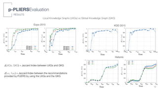

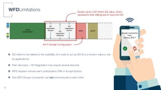
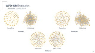
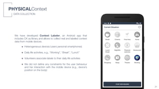
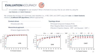
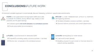
![๏ We compared WFD-GM with a Baseline protocol
๏ We implemented both WFD-GM and Baseline in the ONE opportunistic simulator
๏ Parameters estimation with real devices
0 10 20 30
Hour
0
0.2
0.4
0.6
0.8
1
Batterylevel
Group size: 2
Group size: 20
Intermediate
0 10 20 30
Hour
0
0.2
0.4
0.6
0.8
1
Batterylevel
Group size: 2
Group size: 20
Intermediate
Predicted battery depletion
- GO w/o clients + Service Discovery: 20% every 5h
- Groups of [1,4] clients that continuously send msgs to
each other. Then, we used a linear regression model to
estimate the power consumption in larger groups.
GOs Clients
In simulations: rand(4,15) max clients for each node
SETUP
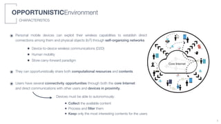
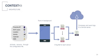
WFD-GMEvaluation
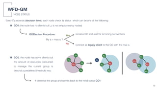
• GO election: node with the highest MAC address
• The GO maintains its role until the end of its resources or in case of out-of-range
• Limited number of clients - e.g., LG Nexus 5 (4 clients), HTC Nexus 5X (10+ clients)
• Battery depletion
21](https://image.slidesharecdn.com/phddefense-190618111514/85/Context-aware-Recommender-Systems-for-Opportunistic-Environments-32-320.jpg)
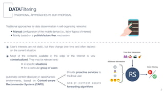
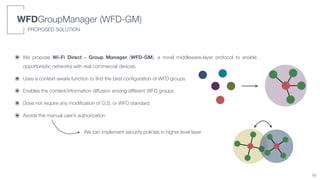
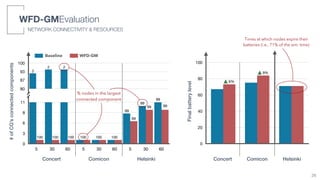
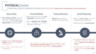
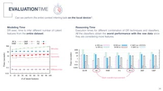
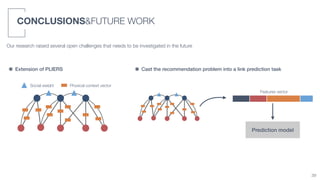
![ComiCon
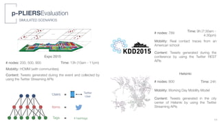
# nodes: 2000
Mobility: [0,1.5] m/s - ShortestPath
575 POIs (e.g., stands, eateries)
Each node waits from 10min to 1h at
each POI (e.g., queues)
Time: 4 h
Helsinki
# nodes: 4000
Mobility: Working Day Mobility Model
Time: 24 h
Concert
# nodes: 1000
Mobility: fixed positions
Time: 3 h
Main Stage
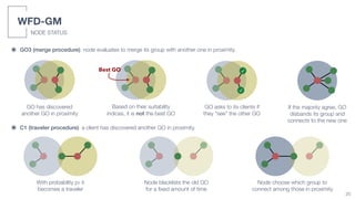
We simulated 3 application scenarios with different numbers of nodes (users) and different mobility patterns
SIMULATED SCENARIOS
WFD-GMEvaluation
22](https://image.slidesharecdn.com/phddefense-190618111514/85/Context-aware-Recommender-Systems-for-Opportunistic-Environments-33-320.jpg)


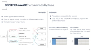
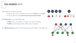
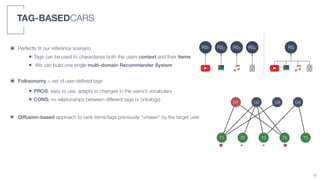
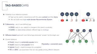
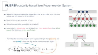
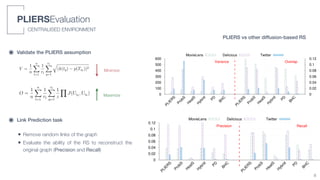
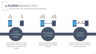
The document summarizes a doctoral thesis on context-aware recommender systems for opportunistic environments. Key points: 1) The thesis proposes a novel context-aware recommender system (CARS) solution designed specifically for opportunistic environments where devices can communicate directly. 2) A tag-based approach is presented that uses user-defined tags to characterize both user context and item information, allowing a single multi-domain recommender system to be built. 3) An algorithm called PLIERS is introduced that recommends items based on tag popularity in a way that does not require parameter tuning and increases neither computational complexity nor recommendation bias.


