2. 104104-2 Görling et al. J. Chem. Phys. 128, 104104 2008
corresponding occupied and unoccupied HF orbitals from a
given orbital basis set, form a linearly independent set. Oth-erwise,
if the products of occupied and unoccupied HF orbit-als
are linear dependent then we show that xOEP schemes, in
general, do not deliver exactly the corresponding ground
state HF energies. Note that Staroverov et al. employed basis
sets of contracted even-tempered primitive Gaussian func-tions
that are formally, i.e., with respect to an infinite com-putational
accuracy, as well as effectively, i.e., with respect
to the actual computational accuracy, linearly independent,
and that for those basis sets the above statement of theirs,
regarding the equality of the xOEP and HF energy, indeed
applies. Note also that they anticipate our results, to some
extent, in that they also concern themselves with linear de-pendencies.
However, our focus is entirely on just orbital
basis products by themselves, and this orientation is crucial
for our analysis.
Secondly, we show that in order to get a physically
meaningful KS exchange potential as a functional derivative
of the exchange energy with respect to the electron density,
an xOEP scheme has to be set up in a way that it represents
a KS method. For instance, in order to adequately describe
the virtual orbitals, the orbital basis has to be comprehensive
enough for the given auxiliary basis. If xOEP schemes are set
up thusly then they are of great usefulness in practice as
demonstrated, e.g., by numerically stable plane wave xOEP
procedures for solids4–8 and, very recently, by a numerically
stable Gaussian basis set approach for molecules.9
It will turn out to be important in this context to distin-guish
between OEP and KS methods and, in particular, be-tween
xOEP and exchange-only KS methods. In order to
clarify this distinction we first concentrate on real space rep-resentations
that correspond to the limit of complete basis
sets and that are the representations used in the original deri-vations
and formulations of OEP Refs. 10 and 11 and KS
methods. OEP methods are characterized by the fact that the
orbitals are eigenstates of a one-particle Schrödinger equa-tion
with an optimized effective potential that is a local mul-tiplicative
potential. Subsequently also the OEP exchange
potential is a local multiplicative exchange potential. This
distinguishes OEP methods from the HF method that con-tains
a nonlocal exchange potential. Within KS methods the
orbitals are eigenstates of a one-particle Schrödinger equa-tions
with a KS effective potential defined as the functional
derivative of the noninteracting kinetic energy, i.e., the ki-netic
energy of the occupied KS orbitals, with respect to the
electron density. The KS exchange potential is given as the
functional derivative of the KS exchange energy with respect
to the electron density. Because functional derivatives with
respect to the electron density are local functions the KS
effective potential as well as the KS exchange potential, by
definition, are local multiplicative potentials. In a real space
representation the OEP method is a KS method and the term
xOEP method can be used synonymously to the term
exchange-only KS method.2 Moreover the Hohenberg–Kohn
theorem applies and all KS and OEP potentials are unique up
to an additive constant.
For a representation within a finite orbital basis set the
problem arises that, given the basis set representation of a
potential, i.e., given the corresponding matrix representing
the potential, it is not possible to distinguish between local
multiplicative and nonlocal operators. Thus it is not clear a
priori how to properly define OEP or KS methods. The defi-nition
for OEP methods adopted by Staroverov et al. in Ref.
1 and also in this work is to define OEP methods as methods
with an optimized effective potential that is represented in
the orbital basis by a matrix containing matrix elements ob-tained
as real space integrals of orbital basis functions with a
local multiplicative potential. Note, however, that a matrix
obtained in this way may be identical to matrix representa-tions
of a nonlocal operator and that different local multipli-cative
potentials may have the same matrix representation,12
i.e., the Hohenberg–Kohn theorem no longer holds.13 As a
consequence xOEP methods can yield the HF energy and can
do so for more than one effective potential if products of
orbital basis functions or, at least, products of occupied times
unoccupied orbitals are linearly independent. This leads to
the seemingly paradoxical finding of Staroverov et al.
Proper basis set KS methods14 must be set up in a way
that they yield unique KS effective and exchange potentials
that converge toward the corresponding potentials of a real
space representation. Finite basis set OEP methods, however,
do not always obey this criterion and thus are not always KS
methods. In particular, finite basis set xOEP methods do not
always represent exchange-only KS methods. This means
that within finite basis set representations the terms OEP and
xOEP method are more general than the terms KS and
exchange-only KS method, respectively. Only certain special
basis set OEP or xOEP methods that are set up properly as
described below represent KS or exchange-only KS methods
and are physically meaningful. Other basis set OEP or xOEP
methods may be technically correct OEP methods but they
do not represent physically meaningful methods. This is one
explanation for the seemingly paradoxical finding of
Staroverov et al. that for finite basis sets their xOEP calcu-lations
always yielded the HF total energy and that the cor-responding
xOEP exchange potentials do not need to be
unique, while in a real space representation the xOEP total
energy lies above the HF one and the xOEP exchange poten-tial
is unique, up to an additive constant: For finite orbital
basis sets with linearly independent products of orbital basis
functions, the requirements to yield a total energy that is
higher than the corresponding HF total energy and a unique
exchange potential only would hold true for exchange-only
KS methods. However, the basis set xOEP calculations of
Staroverov et al. do not represent exchange-only KS calcu-lations
and thus are allowed to yield the HF total energy and
more than one exchange potential. In Appendix B we give a
derivation of basis set xOEP methods that completely avoids
any real space representations and demonstrates that basis set
xOEP methods are not necessarily exchange-only Kohn–
Sham methods.
An understanding of the apparent energy paradox uti-lizes
the constrained-search approach,15 where we shall ana-lyze
the energetics during the transition from the finite to the
complete basis situation. We shall see how, perhaps counter-intuitively,
the addition of orbital basis functions to an xOEP
calculation can actually raise not lower the xOEP energy
Author complimentary copy. Redistribution subject to AIP license or copyright, see http://jcp.aip.org/jcp/copyright.jsp
3. 104104-3 Exchange optimized potential and KS methods J. Chem. Phys. 128, 104104 2008
because of the onset of orbital pair linear dependencies!
Also, an alternative simple proof of the result of Ref. 1 is
presented in Sec. II A that employs the fact that only one
single Slater determinant yields any electron density within
an orbital basis when orbital products are linearly indepen-dent.
II. RELATION OF xOEP AND HF ENERGIES
WITHIN FINITE BASIS SET METHODS
We start by briefly reconsidering the xOEP approach of
Staroverov et al.1 that showed that xOEP methods may yield
the HF total energy for certain choices of basis sets. The
relevant Hamiltonian operators are the HF Hamiltonian op-erator,
i.e., the Fock operator,
H ˆ
HF = − 1
NL 1
22 + vextr + vHr + vˆ x
and the xOEP Hamiltonian operator
H ˆ
xOEP = − 1
22 + vsr = − 1
22 + vextr + vHr + vxr. 2
Atomic units are used throughout. In Eqs. 1 and 2, vextr
denotes the external potential, usually the electrostatic poten-tial
of the nuclei, vHr is the Hartree potential, i.e., the Cou-lomb
potential of the electron density, vxr is the local mul-tiplicative
xOEP exchange potential, vsr=vHr+vxr
NL is the non-local
+vextr is the effective xOEP potential, and vˆ x
exchange operator with the kernel
NLr,r =
vˆ x
r,r
r − r
. 3
Here r,r designates the first-order density matrix. In the
HF-Hamiltonian operator of Eq. 1 the first-order density
matrix occurring in the nonlocal exchange operator of Eq.
3 equals the HF first-order density matrix HFr,r and the
nonlocal exchange operator subsequently equals the HF ex-change
operator. For simplicity we consider closed shell sys-tems
with non-degenerate ground states. In this case, orbit-als,
first-order density matrices, and basis functions can all
be chosen to be real valued.
Next we introduce an orbital basis set of dimension
N. The representations of the HF and xOEP Hamiltonian
operators in this basis set are
NL + Vext 4
HHF = T + VH + Vx
and
HxOEP = T + Vs = T + VH + Vx + Vext, 5
NL, and Vx are de-fined
respectively. The matrices T, VH, Vext, Vx
by the corresponding matrix elements T=
−1
2 , VH,= vH2 , Vext,= vext , Vx,NL
NL , and Vx,= vx , respectively, and by
= vˆ x
Vs=VH+Vx+Vext. Because the orbital basis functions are
real valued all matrices are symmetric
Now we expand the xOEP exchange potential in an aux-iliary
basis set f p of dimension Maux, i.e.,
Maux
vxr =
p=1
cpf pr. 6
The auxiliary basis set, of course, shall be chosen such that
its basis functions are linearly independent. The crucial ques-tion
arising now is how many and what types of matrices Vx
representing the xOEP exchange potential can be constructed
for a given auxiliary basis set f p. This question was an-swered
in Ref. 12. First we consider the case when the M
=1/2NN+1 different products rr of orbital basis
functions are linearly independent. In this case, if Maux=M
and the auxiliary basis functions span the same space as the
products of the orbital basis functions, then any symmetric
matrix Vx can be constructed in a unique way by determining
appropriate expansion coefficients cp for the exchange poten-tial.
The reason is that the determination of the Maux=M
expansion coefficients cp for the construction of the M
=Maux different matrix elements of the symmetric matrix Vx
leads to a linear system of equations
Ac = y 7
of dimension MMaux with
A,p = f p 8
and
y = Vx, 9
for the coefficients cp that is nonsingular and thus has a
unique solution.12 In Eq. 7, A is an MMaux matrix that
contains the overlap matrix elements f p . The first in-dex
of A, i.e., , is a superindex referring to products of
orbital basis functions, while the second index k refers to
auxiliary basis functions. The vector c collects the expansion
coefficients of Eq. 6 for the exchange potential and the
right-hand side y, a vector with superindices , contains the
M=NN+1 /2 independent elements of an arbitrarily chosen
matrix Vx. If we choose Vx to be equal to the matrix repre-sentation
of an arbitrary nonlocal operator with respect to the
orbital basis set then Eqs. 6 and 7 define a local potential
with the same matrix representation. This demonstrates that a
distinction of local multiplicative and nonlocal operators is
not clearly possible for orbital basis sets with linearly inde-pendent
products of orbital basis functions.
If MauxM and the space spanned by the auxiliary func-tions
contains the space spanned by the products of orbital
functions then12 an infinite number of sets of coefficients cp
lead to any given symmetric matrix Vx. The real space xOEP
exchange potentials vxr corresponding according to Eq. 6
to these sets of coefficients cp are all different but all repre-sent
local multiplicative potentials. Next we construct xOEP
Hamiltonian operators Eq. 2 by adding these different
xOEP exchange potentials to always the same external and
Hartree potential. The resulting effective xOEP potentials in
real space, i.e., the vsr are all different. Nevertheless the
resulting basis set representations HxOEP of the correspond-ing
xOEP Hamiltonian operators are all identical because the
basis set representations Vx of the different exchange poten-tials
vxr, by construction, are all identical. As a conse-
Author complimentary copy. Redistribution subject to AIP license or copyright, see http://jcp.aip.org/jcp/copyright.jsp
4. 104104-4 Görling et al. J. Chem. Phys. 128, 104104 2008
quence the xOEP orbitals resulting from diagonalizing the
xOEP Hamiltonian matrix HxOEP and subsequently also the
resulting ground state electron densities are identical in all
cases. We thus have a situation where different local multi-plicative
xOEP potentials vsr lead to the same ground state
electron density. This seems to constitute a violation of the
Hohenberg–Kohn theorem. Indeed it was shown in Ref. 13
and discussed in Ref. 12 that the Hohenberg–Kohn theorem
does not hold for finite orbital basis sets in its original for-mulation,
i.e., that different local potentials, e.g., local poten-tials
obtained by different linear combinations of auxiliary
basis functions, must lead to different ground state wave
functions and thus different ground state electron densities.
We will come back to this point later on. Finally, if Maux
M then not all symmetric matrices Vx can be constructed
from a local xOEP exchange potential given by an expansion
Eq. 6.
In their xOEP approach Staroverov et al.1 can expand
the xOEP exchange potential in Maux=M auxiliary basis
functions and determine the coefficients such that the result-ing
NL. If
matrix Vx exactly equals the HF exchange matrix Vx
additionally the xOEP Hartree potential is set equal to the HF
one then the resulting HF and xOEP Hamiltonian operators
are identical. Subsequently also the HF and xOEP orbitals,
the ground state electron densities, and the ground state en-ergies
are identical. Because the HF and the xOEP electron
densities turn out to be identical, the Coulomb potential of
this density can equally well be considered as a HF or a
xOEP Hartree potential. It follows immediately that the local
exchange potential constructed in this way is the xOEP ex-change
potential: The HF total energy is the lowest total
energy any Slater determinant can yield. Thus if a local mul-tiplicative
potential leads to this total energy, it is clearly the
optimized effective potential defined as the potential that
yields the lowest total energy achievable by any local multi-plicative
potential. The xOEP ground state energy resulting
from this construction equals the corresponding HF energy.
Moreover by enlarging the number of auxiliary basis func-tions,
resulting in MauxM, not only one optimized ex-change
potential leading to the HF energy but infinitely
many can be constructed.
Staroverov et al. obtained the HF energy in their xOEP
scheme even if the number of auxiliary functions only
equaled the product Mov of occupied and virtual orbitals.1
Indeed this case constitutes the first and most important ver-sion
of their approach that is also of greatest interest for its
practical implementations. In this case a similarity transfor-mation
of the HF and the xOEP Hamiltonian matrices and
their constituents is carried out in order to obtain representa-tions
of all matrices with respect to the HF orbitals. Then it is
sufficient to choose the expansion coefficients of the xOEP
exchange potential such that only the occupied-virtual block
of the xOEP exchange matrix equals that of the HF exchange
matrix. The resulting xOEP Hamiltonian matrix then may
differ from the HF Hamiltonian matrix in the occupied-occupied
and the virtual-virtual block, but this merely leads
to unitary transformations of the occupied and virtual orbit-als
among themselves and thus does not change the ground
state energy or the electron density.
For a finite basis set situation it is straightforward to
show that the occupied-virtual block of the exchange matrix
equals that of the HF exchange matrix if the products of
occupied and unoccupied orbitals are linearly independent
and if the xOEP equation
occ.
4
i
unocc.
a
i
rar
avxi
i − a
occ.
= 4
i
unocc.
a
i
rar
NLi
avˆ x
i − a
10
is obeyed pointwise. Equation 10 represents the xOEP
equation that was originally derived to determine the exact
real space xOEP exchange potential10,11 for a full infinite set
of orbitals resulting in a real space representation. In Eq. 10
i
and a denote occupied and unoccupied xOEP orbitals,
i
respectively, with eigenvalues i and a, where, of course,
the unoccupied orbitals form an infinite set. Both sides of Eq.
10 are linear combinations of products rar of occu-pied
and unoccupied xOEP orbitals with coefficients
avxi
NLi
/ i− a and avˆ x
/ i− a, respectively.
Now let us consider the special case of a finite basis OEP
calculation, where the orbitals and the local exchange poten-tial
vx are made to satisfy Eq. 10. Then, if the products
i
rar are linearly independent then the two linear com-binations
can only be identical if the coefficients multiplying
the products are all identical. This, however, requires that
avxi
NLi , i.e., that the occupied-virtual block
=avˆ x
of the xOEP exchange matrix equals that of the correspond-ing
exchange matrix of a nonlocal exchange operator of the
form of the HF exchange operator. Replacement of the xOEP
exchange matrix by the matrix of the nonlocal exchange op-erator
thus again leads only to a unitary transformation of the
occupied and virtual orbitals among themselves. Therefore
the corresponding xOEP determinant would be interpreted as
the HF determinant. In the constrained-search analysis to fol-low,
we shall consider the general finite basis OEP situation,
where Eq. 10 is not necessarily satisfied pointwise. In any
case, it is interesting that for the real space situation Eq. 10
implies directly that the occupied-virtual products are lin-early
dependent because for the real space situation the
xOEP energy differs from the HF energy.
Next we consider the crucial point what happens if the
products of orbital basis functions i
rar are linearly
dependent. To that end we refer to the equation
A˜
c = y˜ , 11
which is a matrix equation of the form of Eq. 7, however,
of different dimensions, MovMaux instead of MMaux
with Mov denoting the number of occupied times unoccu-pied
orbitals and with matrix elements given by
A˜
ia,p = i
af p 12
and
y˜ai = i
NLa . 13
vˆ x
If Eq. 11 can be solved then the exchange potential is de-termined
such that the occupied-virtual block of the ex-
Author complimentary copy. Redistribution subject to AIP license or copyright, see http://jcp.aip.org/jcp/copyright.jsp
5. 104104-5 Exchange optimized potential and KS methods J. Chem. Phys. 128, 104104 2008
change matrix equals that of the HF exchange matrix. How-ever,
a of occupied times unoccupied
if the products i
orbitals are linearly dependent then the rows of the matrix A˜
of Eq. 11 are linearly dependent, thus the rank of the matrix
A˜
is lower than Mov, and as consequence Eq. 11, in gen-eral,
has no solution.
For a further argument, observe that for linear dependent
products i
rar of occupied times unoccupied orbitals,
there exists at least one linear combination of such products
that equals zero
0 =
ia
aiai
rar. 14
In Eq. 14 the aia denote the coefficients of that linear com-bination.
The corresponding sum of matrix elements of Vx
also equals zero, i.e.,
0 = drvxr
ia
aiai
rar =
ia
aiai
vxa 15
for any choice of expansion coefficients cp in Eq. 6 because
the product of any local function and thus of any xOEP
exchange potential vxr with the sum Eq. 14 equals zero.
The products i
rar for two different arguments r and
r, on the other hand, are always linearly independent be-cause
the occupied orbitals i
, as well as the unoccupied
i
orbitals a, are linearly independent among each other.
Therefore the linear combination
iaaiarar cannot be
identical to zero for all values of the arguments r and r, and
it would also be expected that the integral of this linear com-bination
with HFr,r / r−r, i.e., with the kernel of the
nonlocal HF exchange operator, in general, is not equal to
zero, i.e., in general,
0
ia
aiai
HFa . 16
vˆ x
Comparison of Eqs. 15 and 16 implies that, in general,
the exchange matrices Vx and VNL x
are different no matter
how the expansion coefficients cp of the xOEP exchange
potential, Eq. 6, are chosen. This suggests that, in general,
neither the xOEP scheme of Ref. 1 nor any other leads to an
xOEP Hamiltonian operator that equals the HF Hamiltonian
operator if the orbital basis products are linearly dependent.
If we consider the first basic version of Ref. 1’s xOEP
scheme that refers only to the occupied-virtual block of the
xOEP and HF exchange matrices, then by completely analo-gous
arguments it follows that this scheme only works if the
products of occupied and unoccupied HF orbitals are linearly
independent. However, if the products of occupied and un-occupied
HF orbitals are linearly dependent then, in general,
it is not possible to obtain the HF ground state energy via an
xOEP scheme.
We realize the fact that 0
iaaiai
rar does not
necessarily dictate with certainty the shown integrated Eq.
16. Partly with this in mind, we now elucidate the entire
energy situation from a constrained-search perspective. We
shall then discuss the question of how products of basis func-tions
can be linearly dependent.
A. Constrained-search analysis
In this section, complete freedom in the xOEP potentials
is assumed. We start with an alternative proof that the xOEP
ground state energy ExOEP must equal the HF ground state
energy EHF in their common finite orbital basis, when there is
no linear dependence in the products of orbital basis func-tions.
To accomplish this we appeal to the work of
Harriman.13 He showed that only one first-order density ma-trix
may yield any density generated by a given finite orbital
basis whose basis products form a linearly independent set.
This means that since an idempotent first-order density ma-trix
uniquely fixes a corresponding single Slater determinant,
it follows that only one single determinant, constructed from
a given finite orbital basis whose products are linearly inde-pendent,
may yield a density that is constructed from this
same basis. Consequently, with use of a common finite or-bital
basis set, the xOEP single determinant must equal the
HF single determinant if there exists at least one local poten-tial
such that its ground state density is the same as the
Hartree–Fock density. That means it is only required that the
HF density is noninteracting v representable with respect to
the orbital basis set. That at least one such local potential
exists when the basis products are linearly independent, as
discussed above, follows from Ref. 12 and was shown in
practice by Staroverov et al.1
What happens when the products are not linearly inde-pendent?
Due to the idempotency property of the first-order
density matrix for a single determinant, a density generated
from a given finite orbital basis could still generate a unique
determinant if the basis products are linearly dependent, pro-vided
that this linear dependency is mild enough as in the
sense of Refs. 13 and 16. However, by Sec. II in Ref. 16, if
the number of linearly independent products in the orbital
basis becomes smaller than the number of occupied times
unoccupied orbitals, the “critical number” or “critical point,”
then the situation changes dramatically in that more than one
single determinant will yield the same density from the given
basis set. In other words, the number of linearly independent
products must remain at least as large as the critical number
for a density to be generated by a unique determinant in the
basis. Otherwise, we do not have the equality ExOEP=EHF.
Instead, we have the inequality ExOEPEHF, which arises
from the following contradiction.
Assume that the xOEP determinant
xOEP equals the HF
determinant
HF through respective optimizations in their
common finite orbital basis set. Then it follows that their
densities must be the same. But, from a constrained-search
analysis,17 the xOEP determinant
xOEP would yield this HF
density and minimize, within this common basis, just the
expectation value
T ˆ
of the kinetic energy, while the
HF determinant
HF yields this HF density and minimizes,
within the common basis, the expectation value
T ˆ
+V ˆ
ee
of the kinetic energy plus the electron-electron re-pulsion
energy. Here T ˆ
denotes the many-electron kinetic
energy operator, V ˆ
ee the corresponding electron-electron re-pulsion
operator, and
Slater determinants that yield the HF
density. Equivalently, the xOEP determinant would yield the
Author complimentary copy. Redistribution subject to AIP license or copyright, see http://jcp.aip.org/jcp/copyright.jsp
6. 104104-6 Görling et al. J. Chem. Phys. 128, 104104 2008
HF density and minimize
H ˆ
−V ˆ
ee
while the HF deter-minant
yields this HF density and of course minimizes
H ˆ
. HereH ˆ
denotes the many-electron Hamiltonian op-erator.
Because the Slater determinants
xOEP and
HF
would minimize different expectation values, i.e.,
and
+ˆ
V ˆ
T ˆ
T ee
, respectively, the two determinants would
be different, in general, leading to a contradiction of the ini-tial
assumption that the two determinants are the same, and
the inequality ExOEPEHF thus follows for this common fi-nite
orbital basis case. However, there is only one possible
determinant
that yields the HF density from a given finite
basis when the basis products are linearly independent or the
extent of linear dependency is weak. In this case both mini-mizations
yield this one Slater determinant simply because
both minimization only run over one Slater determinant.
Thus there is no contradiction and the finite basis set conclu-sion
of Staroverov et al. follows in that the equality ExOEP
=EHF applies. Hence we are now able to provide a resolution
of the xOEP energy paradox1 from a constrained-search per-spective:
For a finite basis set case, no matter how large the
basis, ExOEP equals EHF provided that the orbital basis prod-ucts
form a linearly independent set or if the number of lin-early
independent basis products remains at least as large as
the critical number. However, in going from any starting fi-nite
basis set to the complete basis set limit, ExOEP becomes
greater than EHF along the way because as more and more
basis orbitals are added to the finite basis set, the onset of
sufficient linear dependency eventually occurs when the
number of linearly independent orbital basis products falls
below the critical number. See Appendix A for a proof that
the products of a complete basis are linearly dependent.
We have provided an explanation for what might very
well seem counterintuitive to the reader without knowledge
of the analysis provided here. As one keeps adding more and
more orbital basis functions, both EHF and ExOEP, at first,
decrease and continually remain equal to each other. Even-tually
in the addition of orbital basis functions, however, EHF
and ExOEP start to differ from each other and EHF keeps de-creasing,
while the behavior of ExOEP depends on the chosen
orbital basis set and it might actually be that ExOEP rises! The
latter behavior, for example, occurs if the exact HF orbitals
as they correspond to a real space representation are them-selves
chosen as the basis set. If the basis set is restricted to
the occupied HF orbitals, EHF and ExOEP are of course equal.
If unoccupied HF orbitals are added to the basis set, EHF
remains unchanged. In contrast, eventually ExOEP raises. The
cause, of course, is the eventual appearance of sufficient lin-ear
dependence.
Note that numerical illustration of the above finite basis
constrained-search analysis appeared in Ref. 12 where, for a
common density, it was found that the
that minimizes
T ˆ
+V ˆ ee
was different than the
that minimized
T ˆ
. In effect, sufficient linear dependency was
achieved. Consequently, an OEP calculation with their basis
would not have achieved the HF energy.
B. Creation of linear dependence
Next we consider how products of orbital basis functions
become linearly dependent. As example we consider a plane
wave basis set corresponding to a unit cell defined by the
three linearly independent lattice vectors a1, a2, and a3. The
plane waves representing the orbital basis set G then are
given by
Gr =
1
7. eiGr 17
with
G = b1 + mb2 + nb3 18
and
,n,m Z
and
G
8. Gcut. 19
In Eq. 18, b1, b2, b3 denote three reciprocal lattice vectors
defined by the conditions a ·bm=2
m for ,m=1,2,3. By
Z the space of all integer numbers is denoted, Gcut denotes
the cutoff that determines the size of the plane wave basis
set, and stands for the crystal volume. We have assumed
before that basis functions are real valued. This is not the
case for plane waves. However, we can always obtain a real
valued basis set by linearly combining all pairs of plane
waves with wave vectors G and −G to real-valued basis
functions. This real-valued basis set and the original
complex-valued plane wave basis set are related by a unitary
transformation that does not change any of the arguments of
this paper. All arguments therefore are also valid for the
complex-valued plane wave basis sets considered here and
below. The number M of basis functions roughly equals
4
/3Gcut
3 V/8
3 with V denoting the unit cell volume.
The exact value of M depends on whether reciprocal lattice
vectors G that lie in the immediate vicinity of the surface of
the sphere with radius Gcut have lengths that are slightly
larger or slightly smaller than Gcut. The relation
GrGr = −1eiGreiGr = −1eiG+Gr =
1
9. G+Gr
20
shows that the products of plane waves of the orbital basis
set are again plane waves of the same type with reciprocal
lattice vectors G+G that obey the relation G+G
10. 2Gcut.
Due to the latter relation the number of different products
GG is about eight times as large as the number N of or-bital
basis functions, i.e., equals about 8N. If N8 then
8NN2. In this case the number 8N of different products of
orbital basis functions is smaller than the number N2 of prod-ucts
of orbital functions. Thus some products of orbital func-tions
are equal and thus linearly dependent. For realistic sys-tems
the number of plane wave basis functions is much
larger than 8. In a plane wave framework therefore xOEP
and HF methods, in general, lead to different ground state
energies with ExOEPEHF. Results from plane wave xOEP
Author complimentary copy. Redistribution subject to AIP license or copyright, see http://jcp.aip.org/jcp/copyright.jsp
11. 104104-7 Exchange optimized potential and KS methods J. Chem. Phys. 128, 104104 2008
and HF calculations for silicon discussed below illustrate this
point.
III. RELATION OF xOEP AND EXCHANGE-ONLY
KS METHODS
In this section we show that the xOEP approach of
Staroverov et al.1 does not correspond to an exact exchange
KS method and does not yield a KS exchange potential, ir-respective
of whether or not the products of basis functions
i
of the
chosen orbital basis set are linearly independent. To
this end we consider the xOEP or exact exchange EXX
equation written in a form that slightly differs from that of
Eq. 10,
occ.
unocc.
drXsr,rvxr = 4
a
i
rar
NLi
avx
i − a
.
21
The response function Xs in Eq. 21 is given by
occ.
Xsr,r = 4
i
unocc.
a
i
rarari
r
i − a
. 22
Equation 21 can be derived in completely different
ways, see, e.g., Ref. 18. First, following Refs. 10 and 11, one
can consider the expression of the HF total energy and search
for those orbitals that minimize this energy under the con-straint
that the orbitals are eigenstates of a Schrödinger equa-tion
with an Hamiltonian operator of the form
H ˆ
xOEP = − 1
22 + vxOEPr. 23
The search for these orbitals is tantamount to searching the
optimal effective potential vxOEP, therefore the name opti-mized
effective potential method. The optimized effective
potential vxOEP can always be expressed as
vxOEPr = vextr + vHr + vxr, 24
with the Hartree potential given as the Coulomb potential of
the electron density generated by the orbitals. As shown in
Refs. 10 and 11 the optimized effective potential vxOEP is
obtained if the exchange potential vx of Eq. 24 obeys the
xOEP or EXX equation Eq. 21. The above derivation
shall be denoted as the OEP derivation of the xOEP or EXX
equation.
Alternatively the xOEP or EXX equation Eq. 21 can
be derived within an exact exchange-only KS
framework;18–20 this derivation shall be denoted KS deriva-tion.
The Hamiltonian operator H ˆ
xKS of the exact exchange-only
KS equation is given by Eq. 2 with the effective KS
potential,
vsr = vextr + vHr + vxr. 25
The KS exchange potential in Eq. 25 is defined as the func-tional
derivative of the exchange energy
occ.
Ex = −
i
occ. dr dr
j
i
rjrjri
r
r − r
26
with respect to the electron density , i.e., as
vxr =
Ex
r
. 27
Following Refs. 19 and 20 we now exploit that according to
the Hohenberg–Kohn theorem there exists a one-to-one map-ping
between effective potentials vs and resulting electron
densities . Therefore all quantities that are functionals of the
electron density, here, in particular, the exchange energy, can
be simultaneously considered as functionals of the effective
potential vs. Taking the functional derivative Ex /vsr of
the exchange energy with respect to the effective potential vs
in two different ways with the help of the chain rule yields
dr
Ex
r
r
vsr
occ. dr
=
i
Ex
i
r
i
r
vsr
. 28
The functional derivative r /vsr equals the re-sponse
function Eq. 22 and the right-hand side of Eq. 28
equals the right-hand side of the xOEP or EXX equation Eq.
21. Furthermore the response function Xs is symmetric in
its arguments for real valued orbitals. Therefore Eq. 28 is
identical to the OEP or EXX equation Eq. 21. This shows
that the exchange potentials arising in the xOEP and the
exact exchange-only KS schemes and subsequently the
xOEP and the exact exchange-only KS schemes itself are
identical. Another derivation of the xOEP or EXX equation,
again within the KS framework, invokes perturbation theory
and exploits the requirement that the first-order correction of
the KS density due to the electron-electron interaction, has to
vanish.20 Thus the xOEP or EXX equation can be derived in
different ways within a KS framework.18 A crucial point,
however, is that all derivations within a KS framework rely
on real space representations in the sense that a local multi-plicative
exchange potential, i.e., a potential given in real
space, is required and that the exchange potential is defined
in real space as functional derivative of the KS exchange
potential Ex /r. Thus the above conclusion that the
xOEP and the exact exchange-only KS schemes are equiva-lent
holds only in real space, i.e., if all quantities are repre-sented
in real space. Calculations, however, are usually car-ried
out in basis sets, and we will show next that in this case
an xOEP and an exact exchange-only KS scheme, in general,
are not equivalent.
The xOEP or EXX equation Eq. 21 turns into the
matrix equation
Xsc = t 29
for the coefficient vector c determining the exchange poten-tial
according to Eq. 6 with matrix and vector elements
occ.
Xs,pq = 4
i
unocc. i
a
f pa afqi
a − s
30
and
occ.
tp = 4
i
unocc. i
a
NLi
f pa avx
i − a
, 31
if an auxiliary basis set f p is introduced to represent the
response function, the exchange potential, and the right-hand
Author complimentary copy. Redistribution subject to AIP license or copyright, see http://jcp.aip.org/jcp/copyright.jsp
12. 104104-8 Görling et al. J. Chem. Phys. 128, 104104 2008
side of the EXX equation Eq. 21. For simplicity we as-sume
at this point that the auxiliary basis set is an orthonor-mal
basis set. This is actually the case for plane wave basis
sets but not for Gaussian basis sets. However, without chang-ing
the following arguments we can assume that we have
orthonormalized any auxiliary Gaussian basis set.
As long as the orbitals are represented in real space there
is an infinite number of them and the summations over un-occupied
orbitals in the response function Eq. 22 and the
right-hand side of the xOEP or EXX equation Eq. 21
remains infinite and complete. For simplicity we assume that
the considered electron system is either periodic and thus
exhibits periodic boundary conditions or, in case of a finite
system, is enclosed in a large but finite box with an infinite
external potential outside the box. Then the number of orbit-als
is infinite but countable. As long as all the infinitely many
orbitals are taken into account in the summation over unoc-cupied
orbitals, the basis set representation of the exchange
potential resulting from the basis set xOEP or EXX equation
Eq. 29 becomes the more accurate the larger the auxiliary
basis set and converges against the real space representation
of the exchange potential and can be interpreted both as ex-act
exchange-only KS or xOEP exchange potential.
This changes dramatically if the orbitals are represented
in a finite orbital basis set. Then, provided a reasonable or-bital
basis set is chosen, the occupied and the energetically
low unoccupied orbitals are well represented. Most of the
energetically higher unoccupied orbitals, however, are not
represented at all simply because a finite orbital basis set
cannot give rise to an infinite number of unoccupied orbitals.
Moreover, the energetically higher orbitals arising in a finite
orbital basis set are quite poor representations of true unoc-cupied
orbitals. Let us now concentrate on the representation
of the response function. The integrals af pi
occurring
in the matrix elements Eq. 30 of the response function
contain the three functions i
, a, and f p. The occupied or-bitals
have few nodes and thus are relatively smooth func-tions.
The energetically low lying unoccupied orbitals still
i
are relatively smooth, the higher ones, however, with an in-creasing
number of nodes and with increasing kinetic energy
become more and more rapidly oscillating. For smooth aux-iliary
basis functions f p the integrals af pi approach
zero if they contain an energetically high unoccupied orbital
a because the product of the smooth functions f p and i
again is a smooth function and the integral of this smooth
product with a rapidly oscillating unoccupied orbital a is
zero due to the fact that any integral of a smooth with a
rapidly oscillating function vanishes. This means that for ma-trix
elements Xs,pq of the response function with two suffi-ciently
smooth functions f p and fq the summation over un-occupied
orbitals in Eq. 30 can be restricted to unoccupied
orbitals a below a certain energy depending on the smooth-ness
of the involved auxiliary basis functions f p and fq. For
sufficiently smooth functions f p and fq the contributing un-occupied
orbitals a thus are well represented in a finite
orbital basis set. Therefore the matrix elements Xs,pq of the
response functions are correct for indices p and q referring to
sufficiently smooth auxiliary basis functions.
For a more rapidly oscillating auxiliary basis function
nonvanishing matrix elements af pi
with energetically
i
high unoccupied orbitals a occur. The energetically high
unoccupied orbitals a, however, are poorly described in the
finite orbital basis set and moreover there are too few of
them. Therefore the matrix elements Xs,pq of the response
functions turn out to be wrong if at least one index refers to
a more rapidly oscillating auxiliary basis functions. Indeed,
if an auxiliary function f p oscillates much more rapidly than
the energetically highest unoccupied orbitals a obtained for
a given orbital basis set, then all matrix elements af p
and thus all corresponding elements Xs,pq of the response
function are erroneously zero. We note in passing that by
similar arguments also the elements tp of the right-hand side
of the matrix OEP equation Eq. 29 turn out to be cor-rupted
if the index p refers to a too rapidly oscillating aux-iliary
basis function.
For a given auxiliary basis set, according to the above
argument, a representation of the response function is correct
only if the orbital basis set is balanced to the auxiliary basis
set in the sense that it describes well unoccupied orbitals up
to a sufficiently high energy. Otherwise an incorrect repre-sentation
of the response function is obtained. The matrix
representation of the response function like the response
function itself is negative semidefinite. This is easily seen if
a matrix element of the type fXsf for an arbitrary function
f is considered. Such a matrix element is obtained by sum-ming
up the contributions occurring in the summation over
occupied and unoccupied orbitals in Eq. 22. Each single
contribution and thus also the complete sum is nonpositive.
Therefore an insufficient orbital basis set leading to too few
energetically high unoccupied orbitals results in eigenvalues
of the response matrix that have a too small magnitude. So-lutions
of the matrix equation Eq. 29 are given by the
product of the inverse of the response matrix with the right-hand
−1t. If Xs contains eigen-values
side of the equation, i.e., by Xs
that are too small, then the corresponding eigenvec-tors
contribute with a too large magnitude to the solution of
Eq. 29. The eigenvectors with too small eigenvalues corre-spond
to rapidly oscillatory functions. Therefore the resulting
exchange potential exhibits rapidly oscillatory features. This
is exactly what is observed in the xOEP scheme of
Staroverov et al.1 If the response matrix even contains eigen-vectors
with eigenvalues that are erroneously zero, then an
infinite number of solutions arise of the matrix equation Eq.
29 corresponding to an infinite number of exchange poten-tials,
which yield, within the finite basis set, the same KS
orbitals.
Therefore if the auxiliary and the orbital basis sets are
chosen unbalanced, e.g., if one chooses a too small orbital
basis set for a given auxiliary basis set or a too large auxil-iary
basis set for a given orbital basis set, then the resulting
response matrix Xs is corrupted and no longer represents a
proper representation of the response function in real space.
In this case the xOEP scheme no longer represents an exact
exchange KS scheme and the resulting exchange potential is
unphysical and no longer represents the KS exchange poten-tial.
However, even in this case the xOEP scheme still is a
proper optimized potential scheme in the sense that it yields
a linear combination of auxiliary basis functions that results
Author complimentary copy. Redistribution subject to AIP license or copyright, see http://jcp.aip.org/jcp/copyright.jsp
13. 104104-9 Exchange optimized potential and KS methods J. Chem. Phys. 128, 104104 2008
in the lowest total energy for this orbital basis set that can be
obtained if the exchange potential shall be a linear combina-tion
of the auxiliary basis functions. While the resulting ex-change
potential is unphysical and does not resemble the KS
exchange potential, it obeys the above requirement of the
xOEP scheme. The reason is that, as shown in Appendix B,
the arguments used for the OEP derivation of the real space
EXX or xOEP equation can also be used if orbital and aux-iliary
basis sets are introduced, whereas no analog to the KS
derivation exists anymore in this case.
IV. EXAMPLES
We now illustrate the arguments of the previous two sec-tions
by specific examples. These examples also demonstrate
that an auxiliary basis set that consists of all products of
occupied and unoccupied orbitals is not balanced to the cor-responding
orbital basis set in the sense that a correct repre-sentation
of the response function and a proper KS exchange
potential cannot be obtained for such an auxiliary basis set.
First, a system of electrons in a box with periodic boundary
conditions and an external potential equal to a constant is
considered. The box shall be defined by corresponding unit
cell vectors ai with i=1,2,3. If the box, i.e., the unit cell
vectors, become infinitely large then the system turns into a
homogeneous electron gas. The KS eigenstates G of such a
system are determined by symmetry and are simple plane
waves G as they are given in Eq. 17. All plane waves with
G vectors of a length smaller than some given constant GF,
i.e., with G
14. GF, shall represent occupied KS orbitals, all
plane waves with GGF represent unoccupied KS orbitals.
The maximal length GF of the vectors G of the occupied
orbitals determines the Fermi level. For the orbital basis set
as well as for the auxiliary basis set we choose plane waves,
G and fG, respectively, again as given in Eq. 17. Thus for
the considered system the special case arises that each orbital
basis function G represents a KS orbital G. Obviously, the
cutoff Gcut of the orbital basis set has to be chosen equal to or
larger than GF.
The matrix representation Xs of the response function in
the considered case is diagonal with diagonal elements,
Xs,GG = 4
G
16. GF
1
G2 − G + G2
. 32
The auxiliary basis set shall be characterized by the cutoff
radius Gcut
aux, i.e., the auxiliary basis set shall consist of all
aux. Note that the auxiliary
plane waves fG with 0G
17. Gcut
function with G=0 that equals a constant function has to be
excluded from the auxiliary basis set because the xOEP or
EXX equation in agreement with the basic formalism deter-mines
the exchange potential only up to an additive constant.
A constant function would be an eigenfunction of the re-sponse
function with zero eigenvalue. Now three cases can
aux
18. Gcut−GF then the correspond-ing
be distinguished: i If Gcut
matrix elements Xs,GG of the response function are ob-tained
with their correct value in a basis set calculation with
an orbital basis set characterized by the cutoff radius Gcut
because all unoccupied orbitals G+G occurring in the sum-mation
in Eq. 32 can be represented by the orbital basis set.
aux
19. Gcut+GF then for the matrix ele-ments
ii If Gcut−GFGcut
Xs,GG with Gcut−GFG
20. Gcut+GF incorrect values
are obtained because some of the unoccupied orbitals G+G
occurring for these matrix elements in the sum in Eq. 32
cannot be represented in the orbital basis set and therefore
are not taken into account. Because all terms in the sum in
Eq. 32 have the same sign the magnitudes of the resulting
matrix elements Xs,GG are too small. iii If Gcut+GFGcut
aux
then the resulting Xs not only contains elements with a too
small magnitude but additionally all matrix elements Xs,GG
with Gcut+GFG are erroneously zero because all of the
unoccupied orbitals G+G occurring in the summation in Eq.
32 cannot be represented in the orbital basis set and there-fore
are not taken into account.
If the auxiliary basis set is chosen to be the space
spanned by all products of occupied and unoccupied orbitals,
then it consists of all plane waves fG with 0G
21. Gcut
+GF, i.e., Gcut
aux=Gcut+GF. Thus the auxiliary basis set is cho-sen
according to the above case ii. Therefore some of the
resulting matrix elements Xs,GG of the response function are
incorrect. This demonstrates that an auxiliary basis set given
by all products of occupied and unoccupied orbitals is not
balanced with the corresponding orbital basis set.
The considered system is special in that the right-hand
side of the xOEP or EXX matrix equation is zero due to the
translational symmetry. Therefore also the resulting ex-change
potential is zero or more precisely equals an arbitrary
constant. If the auxiliary basis set is chosen according to the
above cases i and ii, then a basis set calculation yields the
correct exchange potential, i.e., zero or a constant. If the
auxiliary basis set contains functions according to the above
case iii, however, then the xOEP or EXX matrix equation
erroneously has an infinite number of solutions that equal a
constant plus an arbitrary contribution of auxiliary basis
functions with Gcut+GFG. The reason why the correct
exchange potential is obtained for an auxiliary basis set cho-sen
according to the above case ii despite the fact that in
this case the response function is already corrupted is that for
the special system considered here, as mentioned above, the
right-hand side of the xOEP or EXX matrix equation is zero.
Therefore any values for the diagonal elements Xs,GG that
differ from zero lead to the correct result. However, in gen-eral,
the right-hand side of the xOEP or EXX matrix equation
is not equal to zero and then a response matrix with eigen-values
with erroneously too small magnitudes leads to a
wrong exchange potential that exhibits too large contribu-tions
from those linear combinations of auxiliary basis func-tions
that correspond to the too small eigenvalues of the
response matrix. This is demonstrated in the following ex-ample.
We consider plane wave xOEP calculations for bulk sili-con
carried out with the method of Ref. 4. The integrable
singularity occurring in HF and xOEP exchange energies in
plane wave treatments of solids is taken into account accord-ing
to Ref. 21. The lattice constant was set to the experimen-tal
value of 5.4307 Å. The set of used k-points was chosen
Author complimentary copy. Redistribution subject to AIP license or copyright, see http://jcp.aip.org/jcp/copyright.jsp
22. 104104-10 Görling et al. J. Chem. Phys. 128, 104104 2008
as a uniform 444 mesh covering the first Brillouin zone.
In all calculations, all unoccupied orbitals resulting for a
given orbital basis set were taken into account for the con-struction
of the response function and the right-hand side of
the xOEP equation. EXX pseudopotentials22,23 with angular
momenta l=0,1,2 and cutoff radii, in atomic units, of
rc,Si l=0
=1.8, rc,Si l=1
=2.0, and rc,l=2
Si =2.0 were employed. The
pseudopotential with l=1 was chosen as local pseudopoten-tial.
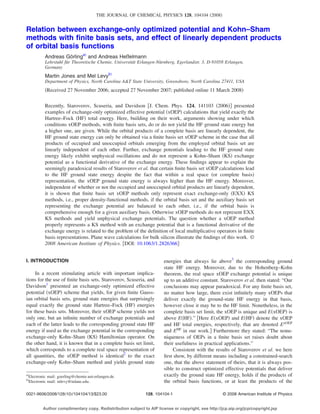
Figures 1 and 2 display xOEP exchange potentials along
the silicon-silicon bond axis, i.e., the unit cell’s diagonal, for
auxiliary basis set cutoffs Ecut
aux of 5.0 and 10.0 a.u. Gcut
aux of
3.2 and 4.5 a.u., and for various different orbital basis set
cutoffs Ecut. Note that in figures and tables instead of the
cutoffs Gcut and Gcut
aux that refer to the length of the reciprocal
lattice vectors of the plane waves the corresponding energy
cutoffs Ecut= 1
2 and Ecut
2Gcut
aux= 1
aux2 are displayed. Figure 1
2 Gcut
shows that the combination of an auxiliary basis set with
cutoff Ecut
aux=5.0 Gcut
aux=3.2 with a orbital basis set with cut-off
Ecut=1.25 Gcut=1.6 leads to a highly oscillating un-physical
exchange potential. The cutoff of the auxiliary basis
set in the considered case is about twice as large as the cutoff
of the orbital basis. This means that the space spanned by the
auxiliary basis is the same as that of all products of occupied
and unoccupied orbitals. In this case the matrix representing
the response function is corrupted and the resulting exchange
potential turns out to be unphysical. With increasing cutoff
Ecut of the orbital basis set the xOEP exchange potentials
converge toward the physical KS exchange potential, more
precisely toward the representation of the physical KS ex-change
aux
potential in an auxiliary basis set with cutoff Ecut
aux=3.2. If the cutoff Ecut of the orbital basis set is
=5.0 Gcut
about 1.5 times as large as the cutoff of the auxiliary basis set
Ecut
aux, i.e., equals 7.5 Gcut=3.9, then the exchange potential
is converged. A further increase of Ecut to Ecut=10.0 Gcut
=4.5 leads to an exchange potential that is indistinguishable
from that for Ecut=7.5 Gcut=3.9 on the scale of Fig. 1.
Figure 2 gives an analogous picture for a cutoff of the aux-iliary
aux=10.0 Gcut
basis set of Ecut
aux=4.5. Again, if the space
spanned by the auxiliary basis set equals that of the product
of occupied and unoccupied orbitals, curve for Ecut=5.0
Gcut=3.2, a highly oscillating unphysical exchange poten-tial
aux then the exchange potential
is obtained. If Ecut
1.5Ecut
is converged toward the representation of the physical KS
exchange potential in an auxiliary basis set with cutoff Ecut
aux
aux=4.5.
=10.0 Gcut
This demonstrates the point that the xOEP scheme only
represents a KS scheme if the orbital basis set is balanced to
the auxiliary basis set. In the case of a plane wave basis set
this requires the energy cutoff Ecut of the orbital basis set to
be about 1.5 times larger than the energy cutoff Ecut
aux of the
auxiliary basis set.
Table I lists for a number of orbital basis set cutoffs Ecut
exchange and ground state energies for series of auxiliary
basis set cutoffs Ecut
aux. Table I shows that the ground state
energies for a given Ecut always decrease with increasing
Ecut
aux even if the values of Ecut
aux are that large that the resulting
exchange potential is unphysical. This demonstrates that the
xOEP scheme remains well defined even if unbalanced basis
sets are used. In this case, however, the xOEP scheme no
FIG. 1. xOEP exchange potential along the silicon-silicon bond axis, i.e.,
the unit cell’s diagonal, for an auxiliary basis set cutoff Ecut
aux=5.0 a.u. and
different orbital basis set cutoffs Ecut. The upper and lower panels differ in
the energy scale. The curve for Ecut=1.25 a.u. is only displayed in the upper
panel.
FIG. 2. xOEP exchange potential along the silicon-silicon bond axis, i.e.,
the unit cell’s diagonal, for an auxiliary basis set cutoff Ecut
aux=10.0 a.u. and
different orbital basis set cutoffs Ecut. The upper and lower panels differ in
the energy scale. The curve for Ecut=5.0 a.u. is only displayed in the upper
panel.
Author complimentary copy. Redistribution subject to AIP license or copyright, see http://jcp.aip.org/jcp/copyright.jsp
23. 104104-11 Exchange optimized potential and KS methods J. Chem. Phys. 128, 104104 2008
xOEP and ExOEP, re-spectively,
aux Maux Ex
longer represents a KS method and the resulting exchange
potential is unphysical and does not represent the KS ex-change
potential. Table I also lists the differences of the
xOEP and HF ground state energies and shows that the
xOEP energy does not converge to the HF energy. In the
combinations Ecut=2.5/Ecut
aux=10.0, Ecut=5.0/Ecut
aux=20.0, and
aux=29.9 the space spanned by the auxiliary basis
Ecut=7.5/Ecut
set roughly equals that of the product of occupied and unoc-cupied
orbitals. The ground state xOEP energies in these
cases are de facto the lowest that can be achieved by the
xOEP method for the given orbital basis set. The fact that
this energy is higher than the HF total energy shows that the
xOEP energy does not reach the HF ground state energy if
the products of occupied and unoccupied orbitals become
linearly dependent as it is usually the case in plane wave
calculations and as it is the case in the presented calculations.
V. SUMMARY
We have given arguments leading to the conclusion that
exchange-only optimized potential xOEP methods, within
finite basis sets, do not yield the Hartree–Fock HF ground
state energy, but a ground state energy that is higher, if the
products of occupied and unoccupied orbitals emerging for
the finite basis set are linearly dependent. This holds true
even if the exchange potential that is optimized in xOEP
schemes is expanded in an arbitrarily large auxiliary basis
set. If, on the other hand, as presented in the surprising re-sults
of Staroverov et al., all products of occupied and unoc-cupied
orbitals emerging for the orbital basis set are linearly
independent of each other, then the HF ground state energy
can be obtained via an xOEP scheme. In this case, however,
exchange potentials leading to the HF ground state energy
exhibit unphysical oscillations and do not represent Kohn–
Sham KS exchange potentials. These findings appear to
explain the seemingly paradoxical results of Staroverov et
al.1 that certain finite basis set xOEP calculations lead to the
HF ground state energy despite the fact that it was shown3
that within a real space representation complete basis set
the xOEP ground state energy is always higher than the HF
energy. A key point is that the orbital products of a complete
basis are linearly dependent, whereas the products of occu-pied
and unoccupied orbitals form a linearly independent set
in the examples of Staroverov et al.
The constrained-search approach was used to understand
the energetics associated with the onset of orbital basis pair
linear dependency in the transition from the linear indepen-dent
to the complete basis real space situation. We saw that
with sufficient linear dependency, the fact that the con-strained
ˆ
V ˆ
T searches of the OEP and HF formulations are asso-ciated
with different operators, +ee in HF and T ˆ
in
OEP, leads to the OEP energy being above the HF energy. In
contrast, the different operator criterion has no effect when
there is no orbital basis pair linear dependency because then
only one wave function yields the density within the basis. It
then follows that the two energies are the same.
Moreover, whether or not the products of occupied and
unoccupied orbitals are linearly independent, we have shown
that basis set xOEP methods only represent exchange-only
EXX KS methods, i.e., proper density-functional methods,
if the orbital basis set and the auxiliary basis set representing
the exchange potential are balanced to each other, i.e., if the
orbital basis set is comprehensive enough for a given auxil-iary
basis set. Otherwise xOEP schemes do not represent
EXX KS methods. We have found that auxiliary basis sets
that consist of all products of occupied and unoccupied or-bitals
are not balanced to the corresponding orbital basis set.
The xOEP method, even in cases of unbalanced orbital and
auxiliary basis sets, works properly in the sense that it deter-mines
among all exchange potentials that can be represented
by the auxiliary basis set the one that yields the lowest
ground state energy. However, in these cases the resulting
exchange potential is unphysical and does not represent a KS
exchange potential. Therefore the xOEP method is of little
practical use in those cases for which it does not represent an
EXX KS method. Remember that, at present, the main rea-son
to carry out xOEP methods in most cases is to obtain a
qualitatively correct KS one-particle spectrum, either for the
purposes of interpretation or as input for other approaches
such as time-dependent density-functional methods. How-ever,
the unphysical oscillations of the exchange-potential of
xOEP schemes with unbalanced basis sets affect the unoccu-pied
orbitals and eigenvalues. Another reason to carry out
xOEP methods that represent EXX KS methods is that the
latter may be combined with new, possibly orbital-dependent,
correlation functionals to arrive at a new genera-
TABLE I. xOEP exchange and ground state energies Ex
and the difference ExOEP−EHF between HF and xOEP ground
state energies for bulk silicon per unit cell for various combinations of
orbital and auxiliary basis sets, characterized by energy cutoffs Ecut and Ecut
aux,
respectively. N and Maux denote the corresponding number of basis func-tions.
All quantities are given in a.u.
Ecut /N Ecut
xOEP ExOEP ExOEP−EHF
2.5/59 2.5 59 −2.1423 −7.4028 0.0054
5.0 137 −2.1434 −7.4033 0.0050
6.0 181 −2.1463 −7.4043 0.0039
7.4 259 −2.1474 −7.4051 0.0031
10.0 411 −2.1479 −7.4053 0.0030
5.0/150 2.5 59 −2.1451 −7.5061 0.0077
5.0 137 −2.1460 −7.5065 0.0073
7.4 259 −2.1468 −7.5069 0.0070
10.0 411 −2.1481 −7.5076 0.0062
14.9 725 −2.1501 −7.5087 0.0051
20.0 1139 −2.1502 −7.5088 0.0050
7.5/274 2.5 59 −2.1482 −7.5269 0.0080
5.0 137 −2.1487 −7.5272 0.0078
7.4 259 −2.1494 −7.5274 0.0075
10.0 411 −2.1495 −7.5275 0.0075
14.9 725 −2.1520 −7.5286 0.0063
24.9 1639 −2.1539 −7.5296 0.0053
29.9 2085 −2.1540 −7.5297 0.0053
10.0/415 2.5 59 −2.1489 −7.5287 0.0081
5.0 137 −2.1494 −7.5290 0.0078
7.4 259 −2.1500 −7.5292 0.0076
10.0 411 −2.1501 −7.5292 0.0076
14.9 725 −2.1505 −7.5294 0.0074
20.0 1139 −2.1511 −7.5296 0.0072
Author complimentary copy. Redistribution subject to AIP license or copyright, see http://jcp.aip.org/jcp/copyright.jsp
24. 104104-12 Görling et al. J. Chem. Phys. 128, 104104 2008
tion of density-functional methods. Also in this case it is
important that xOEP methods represent proper KS methods.
A balancing of auxiliary and orbital basis sets is straight-forward
for plane wave basis sets. In this case xOEP schemes
are proper EXX KS methods if the energy cutoff for the
orbital basis set set is about 1.5 times as large as that of the
auxiliary basis set. This as well as other results of this work
was illustrated with plane wave calculations for bulk silicon.
For Gaussian basis sets on the contrary, a proper generally
applicable and reasonably simple balancing scheme of or-bital
and auxiliary basis sets for a long time could not be
developed despite much efforts.24–29 Numerical grid meth-ods,
on the other hand, so far, could be applied only to
atoms11 and a few very small molecules.30 Therefore effec-tive
exact exchange-only methods like the KLI,31 the “local-ized
Hartree–Fock,”32 the equivalent “common energy de-nominator
approximation” method,33 and the closely related
very recent method of Ref. 34 as well as OEP methods that
add terms smoothing the exchange potential to the total en-ergy
expression35 are in use as numerically stable alterna-tives
that yield results very close to those of full EXX KS
methods. Very recently, however, a numerically stable OEP
method based on Gaussian basis sets with an accompanying
construction and balancing scheme for the involved auxiliary
and orbital Gaussian basis sets was presented.9
There are exact known stringent necessary constraints
for a vx to be consistent with the KS functional derivative
criterion. These constraints include the exchange potential
identity involving the highest occupied KS orbital,36,31 the
virial37 relation Ex=−rr·vxrdr, and vxrrdr
=0, which arises38 simply from the requirement that vx is the
functional derivative of some functional. These constraints
alone would eliminate many vx potentials that do not satisfy
the KS criterion.
APPENDIX A: LINEAR DEPENDENCE OF PRODUCTS
OF BASIS FUNCTIONS OF A COMPLETE BASIS
Let kx be a complete set of functions of a complex
valued variable x such that any arbitrary square integrable
function can be written as a linear combination of the func-tions
in the complete set.We show that the set kxl
x is
linearly dependent.
Using our complete sets, an arbitrary function fx, y of
two complex valued variables x and y may be expanded in
terms of kx and y,
bk,ykx. A1
fx,y =
k
=1
=1
Set y=x to get
bk,xkx. A2
fx,x =
k
=1
=1
Now choose a function fx,x and a nx out of the set
kx such that i limx→fx,x /nx=0 and ii at least
one bk,0 when n and kn. Since fx,x /nx is just
a function of x, we may expand it in terms of the kx,
fx,x
nx
dmmx. A3
=
m=1
Solving for fx,x,
dmmx =
fx,x =nx
m=1
dmmxnx A4
m=1
and equating Eq. A2 with Eq. A4, we get
dmmxnx =
k
m=1
bk,kxx, A5
=1
=1
or by setting k=m,
dmmxnx −
m=1
bm,mxx = 0, A6
m=1
=1
or
dj − bj,n − bn,jnxjx
dn − bn,nnxnx +
j
=1
jn
−
=1
n
m=1
mn
bm,mxx = 0. A7
l
Equation A7 is a linear combination of a subset of
kxx broken up into disjoint components and equated
to zero. If a subset of a set is linearly dependent, then the set
must also be linearly dependent. We show such a case by
contradiction: According to Eq. A7, for the subset
kxl
x appearing in the equation to be linearly in-dependent,
three conditions must be met:
1 dn=bn,n.
2 dj−bj,n−bn,j=0 ∀jN with jn.
3 bm,=0 ∀m,N with mn and n.
But according to our condition on fx,x there is at least one
bm,0 with mn and n, which is a contradiction to
number three of our linear independence criteria. Therefore
kxl
x must be linearly dependent by contradiction,
and therefore kxl
x for all k, lN is linearly depen-dent
because kxl
x is linearly dependent.
One may take the result one step further to show with an
induction argument that for any complete set such as kx
the set defined by i=1
N pix N, i , piN is complete and
linearly dependent.
APPENDIX B: DIRECT DERIVATION
OF THE BASIS SET xOEP EQUATION
If the orbitals and the exchange potential are represented
by basis sets then the OEP derivation10,11 of the real space
xOEP equation Eq. 10 can be adapted in such a way that
it directly yields the basis set xOEP equation Eq. 29 with-out
the need to invoke the real space xOEP equation Eq.
10. In order to show this we consider a basis set represen-tation
HxOEP=T+Vs of a Hamiltonian as it is given in Eq.
5. The energetically lowest eigenvectors ui represent the
Author complimentary copy. Redistribution subject to AIP license or copyright, see http://jcp.aip.org/jcp/copyright.jsp
25. 104104-13 Exchange optimized potential and KS methods J. Chem. Phys. 128, 104104 2008
corresponding occupied orbitals, while the other eigenvec-tors
ua represent the unoccupied orbitals. Any matrix Vs rep-resenting
an effective potential in the orbital basis set can be
written as sum VH+Vx+Vext of the matrix Vext representing
the external potential, the matrix VH representing the Cou-lomb
potential resulting from the occupied orbitals, and a
remainder Vx given by matrix elements Vx,
=
Maux
p=1
cpf p that are determined by a linear combina-tion
of auxiliary basis functions f p, see Eq. 6. The deriva-tive
of the corresponding exchange-only total energy ExOEP
with respect to the coefficients cp is given by
dExOEP
dcp
occ.
= 4
i
unocc.
a
A˜
ia,p
TT + VH + Vx
ua
NL + Vextui
i − a
occ.
= 4
i
unocc.
a
A˜
ia,p
TVx
ua
NL − Vxui
i − a
, B1
with matrix elements A˜
ia,p=i
a f p of Eq. 12. The matrix
A˜
is the one that also occurs in Eq. 11. For the second line
of Eq. B1 it is used that Tui= iS−Vsui= iS−VH−Vx
−Vextui because the coefficient vectors ui representing the
orbitals solve the generalized eigenvalue problem T
+Vsui= iSui, with S being the overlap matrix with respect
to the orbital basis set. Furthermore, it is used that uTa
iSui
=0 due to the orthonormality of the orbitals.
Next we consider the energy ExOEP as function of the
coefficients cp and search the minimum of this function, i.e.,
the minimum of the energy ExOEP. At the minimum the en-ergy
derivatives dExOEP/dcp for all indices p have to be zero.
This means that for each index p an equation
occ.
4
i
unocc.
a
A˜
ia,p
TVxui
i − a
ua
occ.
= 4
i
unocc.
a
A˜
ia,p
NLui
ua
TVx
i − a
B2
holds. The set of equations Eq. B2 is identical to the basis
set xOEP equation Eq. 29 if it is used that the right-hand
side of Eq. B2 equals the elements tp of the vector t on the
right-hand side of the basis set xOEP equation Eq. 29 and
that the left side of Eq. B2 equals the pth element of the
product Xsc, i.e., the pth row of the left side of the basis set
xOEP equation Eq. 29. The latter follows because
uMaux
a
TVxui=
uaVx,ui=
ua
q=1
cqfq ui
Maux
=
q=1
Maux
cq
uaA,qui=
q=1
A˜
ia,qcq with ua and ui de-noting
the elements of ua and ui and with the matrix ele-ments
A,q given by Eq. 8 and because the response ma-trix
Xs of Eq. 29 can be written as Xs=4A˜
T−1A˜
with the
diagonal matrix defined by the matrix elements ia,jb
=ia,jb i− a.
1V. N. Staroverov, G. E. Scuseria, and E. R. Davidson, J. Chem. Phys.
124, 141103 2006.
2V. Sahni, J. Gruenbaum, and J. P. Perdew, Phys. Rev. B 26, 4371 1982.
3 S. Ivanov and M. Levy, J. Chem. Phys. 119, 7087 2003.
4M. Städele, J. A. Majewski, P. Vogl, and A. Görling, Phys. Rev. Lett. 79,
2089 1997.
5M. Städele, M. Moukara, J. A. Majewski, P. Vogl, and A. Görling, Phys.
Rev. B 59, 10031 1999.
6 R. J. Magyar, A. Fleszar, and E. K. U. Gross, Phys. Rev. B 69, 045111
2004.
7 A. Qteish, A. I. Al-Sharif, M. Fuchs, M. Scheffler, S. Boeck, and J.
Neugebauer, Comput. Phys. Commun. 169, 28 2005.
8P. Rinke, A. Qteish, J. Neugebauer, C. Freysoldt, and M. Scheffler, New
J. Phys. 7, 126 2005.
9 A. Hesselmann, A. W. Götz, F. Della Sala, and A. Görling, J. Chem.
Phys. 127, 054102 2007.
10 R. T. Sharp and G. K. Horton, Phys. Rev. 90, 317 1953.
11 J. D. Talman and W. F. Shadwick, Phys. Rev. A 14, 36 1976.
12 A. Görling and M. Ernzerhof, Phys. Rev. A 51, 4501 1995.
13 J. E. Harriman, Phys. Rev. A 27, 632 1983; 34, 29 1986.
14W. Kohn and L. J. Sham, Phys. Rev. 140, A1133 1965.
15M. Levy, Proc. Natl. Acad. Sci. U.S.A. 76, 6062 1979.
16M. Levy and J. A. Goldstein, Phys. Rev. B 35, 7887 1987.
17 See the constrained-search discussion in Ref. 3, which includes appropri-ate
references on the approach in this context.
18 A. Görling, J. Chem. Phys. 123, 062203 2005, and references therein.
19 A. Görling and M. Levy, Phys. Rev. A 50, 196 1994.
20 A. Görling and M. Levy, Int. J. Quantum Chem., Quantum Chem. Symp.
29, 93 1995.
21P. Carrier, S. Rohra, and A. Görling, Phys. Rev. B 75, 205126 2007.
22 E. Engel, A. Höck, and S. Varga, Phys. Rev. B 63, 125121 2001.
23 E. Engel, A. Höck, R. N. Schmid, and R. M. Dreizler, Phys. Rev. B 64,
125111 2001.
24 A. Görling, Phys. Rev. Lett. 83, 5459 1999.
25 S. Ivanov, S. Hirata, and R. J. Bartlett, Phys. Rev. Lett. 83, 5455 1999.
26 S. Hamel, M. E. Casida, and D. R. Salahub, J. Chem. Phys. 114, 7342
2001.
27 L. Veseth, J. Chem. Phys. 114, 8789 2001.
28 S. Hirata, S. Ivanov, I. Grabowski, R. J. Bartlett, K. Burke, and J. D.
Talman, J. Chem. Phys. 115, 1635 2001.
29W. Yang and Q. Wu, Phys. Rev. Lett. 89, 143002 2002.
30 S. Kümmel and J. P. Perdew, Phys. Rev. Lett. 90, 043004 2003.
31 J. B. Krieger, Y. Li, and G. J. Iafrate, Phys. Rev. A 46, 5453 1992.
32F. Della Sala and A. Görling, J. Chem. Phys. 115, 5718 2001.
33 O. V. Gritsenko and E. J. Baerends, Phys. Rev. A 64, 042506 2001.
34V. N. Staroverov, G. E. Scuseria, and E. R. Davidson, J. Chem. Phys.
125, 081104 2006.
35T. Heaton-Burgess, F. A. Bulat, and W. Yang, Phys. Rev. Lett. 98,
256401 2007. F. A. Bulat, T. Heaton-Burgess, A. J. Cohen, and W.
Yang, J. Chem. Phys. 127, 174101 2007.
36M. Levy and A. Görling, Phys. Rev. A 53, 3140 1996.
37M. Levy and J. P. Perdew, Phys. Rev. A3, 2010 1985.
38 H. Ou-Yang and M. Levy, Phys. Rev. Lett. 65, 1036 1990.
Author complimentary copy. Redistribution subject to AIP license or copyright, see http://jcp.aip.org/jcp/copyright.jsp