SlideShare a Scribd company logo
1 of 56
Download to read offline
Shari Friedman
David Gardiner & Associates
Farms Here, Forests There
Tropical Deforestation and U.S.
Competitiveness in Agriculture and Timber
i
Acknowledgements
We greatly appreciate the support of the National Farmers Union and Avoided Deforestation Partners for this
report. We are particularly grateful to NFU president Roger Johnson and Jeremy Peters for their thoughtful
engagement, and ADP’s Founding Partner Jeff Horowitz and Washington Director Glenn Hurowitz for
their contributions.
Many different people helped make this report possible. Jonah Busch, Ph.D. of Conservation International and
Ruben Lubowski, Ph.D. of the Environmental Defense Fund provided invaluable assistance in the development
of the economic models used in the report. Erin Myers Madeira and Andrew Stevenson of Climate Advisers and
Resources for the Future gave extensive and important analytic input.The Union of Concerned Scientists provided
the resources of its Tropical Forest and Climate Initiative to assist in development and review of the report.
Particular thanks go to Douglas Boucher, Ph.D. and Pipa Elias who provided guidance on integration of their
own and other groundbreaking research.
We are also grateful to the many expert reviewers who provided detailed comments and feedback, including
Glenn Bush, Ph.D. of the Woods Hole Research Center, Professor Bruce Babcock at the Center for Agricultural
and Rural Development of Iowa State University, Barbara Bramble of the National Wildlife Federation, Sara
Brodnax of The Clark Group,Toby Janson-Smith of Conservation International, Professor Brian Murray of
Duke University’s Nicholas Institute, Alexia Kelly of the World Resources Institute, Sasha Lyutse of the Natural
Resources Defense Council, Anne Pence of Covington and Burling, Annie Petsonk of the Environmental Defense
Fund, Nigel Purvis of Climate Advisers, Naomi Swickard of the Voluntary Carbon Standard, Michael Wolosin of
The Nature Conservancy and several others.
Carley Corda and her team at Glover Park Group designed the report, and special thanks go to Erik
Hardenbergh, Ryan Cunningham, and Grant Leslie for their help. Olivier Jarda and Caitlin Werrell provided
research support, and Rachel Arends reviewed the design.
ii
About the Author
David Gardiner & Associates prepared the paper on behalf of Avoided Deforestation Partners and the National
Farmers Union. Shari Friedman, Senior Advisor to DGA, served as lead author.
David Gardiner & Associates helps industry, nonprofits and foundations solve energy and climate challenges.
DGA has expertise in climate and energy policy and regulation, as well as tools and strategies for businesses to
reduce emissions, lower costs and create advantages within existing or potential policies. DGA also works with
foundations and NGOs to develop and pursue strategies that advance their climate and energy goals.
Shari Friedman is the President of ASF Associates and Senior Advisor to David Gardiner & Associates. ASF
Associates focuses on climate change policy and private sector strategies. Ms. Friedman has 14 years of experience
in climate change, including policy development, international negotiations and greenhouse gas markets. She has
experience in both the federal government and the private sector. From 1995 to 2001, Ms. Friedman worked on
climate change at EPA, analyzing domestic climate change policies and international competitiveness. From 1998
to 2001, Ms. Friedman was part of the U.S. negotiating team for the Kyoto Protocol, focusing on rules for project-
level trading, particularly the Clean Development Mechanism.
In 2001, Ms. Friedman joined Environmental Enterprises Assistance Fund (EEAF), which managed private
equity funds for environmental businesses. Ms. Friedman left EEAF to create Opus4, now ASF Associates. Ms.
Friedman has a Masters degree in Public Policy from Georgetown University and a B.A. from Tufts University.
iii
Contents
Executive Summary .  .  .  .  .  .  .  .  .  .  .  .  .  .  .  .  .  .  .  .  .  .  .  .  .  .  .  .  .  .  .  .  .  .  .  .  .  .  .  .  .  .  .  .  .  .  .  .  .  .  .  .  .  .  .  .  .  .  .  .  .  .  .  .  .  . 1
I. Background .  .  .  .  .  .  .  .  .  .  .  .  .  .  .  .  .  .  .  .  .  .  .  .  .  .  .  .  .  .  .  .  .  .  .  .  .  .  .  .  .  .  .  .  .  .  .  .  .  .  .  .  .  .  .  .  .  .  .  .  .  .  .  .  .  .  .  .  .  . 6
II. Commodity Change Estimates and Impacts on U.S. Markets .  .  .  .  .  .  .  .  .  .  .  .  .  .  .  .  .  .  .  .  .  .  .  .  .  .  .  . 14
	 a. Soybeans .  .  .  .  .  .  .  .  .  .  .  .  .  .  .  .  .  .  .  .  .  .  .  .  .  .  .  .  .  .  .  .  .  .  .  .  .  .  .  .  .  .  .  .  .  .  .  .  .  .  .  .  .  .  .  .  .  .  .  .  .  .  .  .  . 14
	 b. Vegetable Oil .  .  .  .  .  .  .  .  .  .  .  .  .  .  .  .  .  .  .  .  .  .  .  .  .  .  .  .  .  .  .  .  .  .  .  .  .  .  .  .  .  .  .  .  .  .  .  .  .  .  .  .  .  .  .  .  .  .  .  .  .  . 18
	 c. Beef . .  .  .  .  .  .  .  .  .  .  .  .  .  .  .  .  .  .  .  .  .  .  .  .  .  .  .  .  .  .  .  .  .  .  .  .  .  .  .  .  .  .  .  .  .  .  .  .  .  .  .  .  .  .  .  .  .  .  .  .  .  .  .  .  .  .  .  .  . 21
	 d. Timber  .  .  .  .  .  .  .  .  .  .  .  .  .  .  .  .  .  .  .  .  .  .  .  .  .  .  .  .  .  .  .  .  .  .  .  .  .  .  .  .  .  .  .  .  .  .  .  .  .  .  .  .  .  .  .  .  .  .  .  .  .  .  .  .  .  . 24
III. Financial Impact of Tropical Forest Offsets . .  .  .  .  .  .  .  .  .  .  .  .  .  .  .  .  .  .  .  .  .  .  .  .  .  .  .  .  .  .  .  .  .  .  .  .  .  .  .  .  .  . 28
IV. Conclusion . .  .  .  .  .  .  .  .  .  .  .  .  .  .  .  .  .  .  .  .  .  .  .  .  .  .  .  .  .  .  .  .  .  .  .  .  .  .  .  .  .  .  .  .  .  .  .  .  .  .  .  .  .  .  .  .  .  .  .  .  .  .  .  .  .  .  .  . 29
iv
1
EXECUTIVE SUMMARY
Destruction of the world’s tropical forests by overseas
timber, agriculture, and cattle operations has led to a
dramatic expansion in production of commodities that
compete directly with U.S. products. About 13 million
hectares (32 million acres) of forest are destroyed
every year — mostly in the tropics.1
This deforestation
has allowed large-scale low-cost expansion of timber,
cattle and agricultural production, and has also caused
damage to the environment and forest communities.
Much of this timber and agricultural expansion has
come through practices that do not meet U.S. industry
standards for sustainability, labor practices, and basic
human rights, providing these overseas agricultural
operations a competitive advantage over U.S. producers.
The U.S. agriculture and forest products industries
stand to benefit financially from conservation of
tropical forests through climate policy. Ending
deforestation through incentives in United States
and international climate action would boost U.S.
agricultural revenue by an estimated $190 to $270
billion between 2012 and 2030.This increase includes
$141 to $221 billion in direct benefits from increased
production of soybeans, beef, timber, palm oil and palm
oil substitutes, and an estimated $49 billion* savings
in the cost of complying with climate regulations due
to lower energy and fertilizer costs resulting from the
inclusion of relatively low-cost tropical forest offsets.
Climate legislation currently under consideration
in Congress includes provisions to unlock these
benefits for U.S. agriculture through a combination
of tropical rainforest offsets and by setting aside
allowances for tropical rainforest conservation.
Combined with anticipated comparable action by
other developed countries, these policies aim to cut
tropical deforestation in half by 2020 and eliminate it
entirely by 2030.
This report analyzes the impact of achieving these
conservation goals†
on U.S. production of soybeans,
palm oil substitutes, beef, and timber. Eliminating
deforestation by 2030 will limit revenues for
agricultural expansion and logging in tropical countries,
*	 Analysis of the cost of compliance with climate regulation was done by Climate Advisers. See Section III for more details.
†	 These benchmarks are chosen based on global targets for reduced deforestation.
2
providing a more level playing field for U.S. producers
in global commodities markets. We examine potential
annual effects of a reduction in deforestation as well as
the cumulative effect between 2012 and 2030.
Methodology
This report is a first step in understanding the potential
impacts on U.S. agriculture of deforestation and global
forest conservation efforts. We consider the impact of
reduced production of these commodities on tropical
forest lands and estimate how this reduction would
affect the world market, taking into account resulting
changes in commodity production on non-forest lands
in tropical forest nations, the United States, and other
parts of the world.
We begin by estimating the amount of each
commodity that is produced on formerly forested
land. We consider the impact of a reduction in the
forested land available for agricultural and timber
production in the tropics, without considering the
underlying government policies and measures that
would produce this result. This analysis has been
structured around available data and therefore methods
are specific to each commodity. Assumptions are
outlined in the body of the paper.
We use a partial equilibrium model to estimate the
impact of this reduction on the world market and
the price effects and changes reduced commodity
production from deforested land would have for
revenue for the U.S. agriculture and timber markets. We
use a range of supply and demand elasticities (estimates
of the responsiveness of quantity demanded and
supplied to changes in price) from existing literature
to provide a scope of possible outcomes. In the low
revenue scenario, the United States has a limited
ability to adjust production in response to market price
changes and the rest of the world has a greater ability.
In the high revenue scenario, the United States has a
greater ability to respond to market price changes and
the rest of the world has a more limited ability.
We do not consider cross-elasticities or how the price
increase of one commodity could affect the revenues
of another.This could be a factor for beef revenues if
soybean prices increase and vice versa.These factors
(discussed more in Annex B) are important to drawing
a fuller picture of what would occur under reduced
deforestation scenarios. We aim to provide an initial
concept of the scope of the issue as a basis to move
forward with a fuller analysis. Given time constraints
and the dearth of existing data and analysis on this
topic, this report makes the best possible use of the
resources available. A fuller analysis would incorporate
dynamic economic modeling of price changes,
estimates of technological improvements, changes in
elasticities over time, more disaggregated and detailed
country and regional supply reaction and impacts of
supply changes in one commodity on production of
other commodities.These are recommended areas for
further research.
Impact of Offsets
Allowing international forestry offsets in climate
legislation also affects U.S. agriculture and forestry.
Because these offsets are among the most affordable
means of reducing climate pollution, they would
provide significant savings on electricity, fuel, fertilizer,
and other input costs for the U.S. agriculture, ranching,
Cumulative Revenue Increase
to U.S. Agriculture and TImber Producers
from Ending Deforestation, 2012 – 2030
Commodity 2008 U.S. $ Billion
Soybeans $34.2 – $53.4
Palm Oil and
Palm Oil
Substitutes (1)
$17.8 – $39.9
Beef $52.7 – $67.9
Timber $36.2 – $60.0
Total
Cumulative
$141.0 – $221.3
(1)	 Includes crops for soybean oil, cottonseed oil, sunflower oil and
canola oil
3
and forest products industries.These input costs are
major expenses for the industries analyzed in this
report — the agriculture sector alone spends about
$10 billion just on energy each year.2
Easing near-term
costs of a climate policy allows the sectors to transition
more smoothly to carbon-efficient technologies and
reduce the overall cost.
Allowing capped entities, including energy producers,
to “offset” their emissions by investing in affordable
emissions reduction options such as tropical forest
conservation will reduce permit prices, therefore
keeping energy prices low for farmers, ranchers,
and the forest products industry.Tropical forest
conservation is among the lowest-cost emissions
reduction options available, providing important
savings for the agriculture and forest products
industries. EPA has estimated that the cost of
emissions permits in the House-passed American
Clean Energy and Security Act would be 89%
more expensive if international offsets (the bulk of
which are expected to come from tropical forest
conservation) were excluded.3
Estimates based on
EPA’s analysis of the House-passed American Clean
Energy and Security Act indicate that the inclusion of
international offsets will save the agriculture, forestry,
fishing and timber industries about $4.6 billion per
year and $89 billion between 2012 and 2030.4
With
tropical forest conservation likely to comprise an
estimated 56% of offsets in the years immediately
following implementation of climate legislation
(though more afterwards), this translates into a cost
savings for these industries of approximately $49
billion between 2012 and 20305
(see Section III).
4
T
his paper focuses on the economic impacts of
deforestation — and forest conservation —
on the U.S. agriculture and timber industries.
But what about the impact on people in the rainforest
nations themselves?
Right now, many people in rainforest nations face
a terrible choice. In the absence of incentives for
their protection, forests are worth more dead than
alive. A company or peasant is forced to weigh the
very immediate financial proceeds of cutting down
a forest for timber, agriculture, or ranching against
the damage wrought by deforestation to their own
communities, wildlife, water and the planet — as
well as the lost potential future financial value of the
land as a carbon sink. Even if clearing and burning a
hectare of rainforest only produces ranchland worth
$200 per hectare, many people make the choice to
cut it down anyway — because that deforestation
can, at least in the short run, put food on the table
or boost earnings for a quarterly report to investors.
But that decision comes at a terrible long-term
economic price. Based on recent prices in European
carbon markets, the value of a hectare of rainforest
as a carbon sink is approximately $10,000 a hectare.
Releasing that carbon into the atmosphere by
clearing or burning the forest means sacrificing the
opportunity to realize that value. As a recent World
Bank report put it, “Farmers are destroying a $10,000
asset to create one worth $200.” *
So how will providing financial incentives for the
conservation of forests affect those who are profiting
from deforestation? In most cases, the people cutting
down the forests have the most to gain from conserving
forests. Because incentives to end deforestation are
established to, in part, compensate those who lose
money by bypassing an opportunity to deforest,
the farmers, loggers, and landowners themselves
tend to have the most to gain.They will be the ones
compensated — they can gain income far exceeding
SIDEBAR: The Impact of Deforestation on People in Rainforest Nations
any profits from deforestation, and enjoy enormous
benefits to their local communities and environments.
For instance, in Brazil, many of the ranchers and
farmers most responsible for deforestation have
become advocates of forest conservation programs.
Pilot projects and an increasing recognition of the
high costs of deforestation have convinced many
that they and their communities will become richer
— and also enjoy a better quality of life — through
conserving forests rather than cutting them down.
Perhaps the most prominent embodiment of these new
conservationists is Blairo Maggi, Brazil’s “King of Soy”
— the country’s biggest private landowner, personally
responsible for tens of thousands of acres of forest
destruction, and governor of Mato Grosso province,
ground zero for deforestation. Maggi made his name
throughout the world as an enemy of conservationists
and a vocal ideological defender of deforestation as the
path to riches for himself and the citizens of his state.
Maggi has changed, however. He has recently urged
adoption of policies to conserve the forest — if
the state can find developed country governments
or private companies who will finance forest
conservation, most likely as part of a mandatory
carbon reduction system. Forest conservation
incentives “will be much, much more profitable than
soybeans,” he told Forbes Magazine.†
In addition, even a small carbon incentive can do a
lot to bring production in rainforest nations up to
the environmental and social standards of the United
States and other developed countries.
Protecting forests will also create much needed,
well-paying jobs in developing countries. Forest
conservation requires people: park rangers to patrol
the forest, foresters to measure carbon storage, and
even satellite manufacturers and operators to provide
deforestation monitoring. Reforestation activities
*	 Chomitz, Kenneth. At Loggerheads? Washington, DC: The World Bank, 2007.
†	 Perlroth, Nicole. “Tree Hugger.” Forbes Asia Magazine. December 14, 2009. http://www.forbes.com/global/2009/1214/issues-blairo-maggi-
jungle-conservation-tree-hugger.html
5
that often accompany forest conservation can provide
additional employment opportunities.
Protecting existing forests will also provide a more
sustainable source of jobs in extractive industries
themselves. In places without conservation incentives,
forests are routinely stripped of all their value and
the ground is left as a barren desert that can’t support
communities or jobs. For this reason, many producers in
tropical countries have advocated
establishing carbon incentives that
would rapidly shift production to
more sustainable sources.
In Indonesia, for example, clear
cutting has drastically reduced
the availability of trees to
provide employment in forestry,
including logging. According to
the Indonesian forestry union,
Kahutindo, employment in
forest products has declined by
more than 50 percent in the past
decade, from 2 million workers to
fewer than 1 million today. As a
result, Kahutindo now advocates
conserving existing rainforests
and relying solely on reforestation
to produce fiber. **
There is evidence that this
strategy will work globally
to create well-paying jobs in
the forestry sector. The latest
U.N. Food and Agriculture
Organization State of the Forests
report estimated that switching
to sustainable forest management
would create 10 million good
jobs globally, which would
create a major force against rural
unemployment, underemployment and poverty.††
Benefits in the agricultural and ranching sectors are
likely to be significantly greater, given the greater
economic values. Providing financial incentives for
forest preservation will allow a wide array of people,
from peasants to landowners, to preserve the forests
we all need to fight climate change.
– Glenn Hurowitz
**	 Foster, David. “Indonesia’s Forestry Workers – Another Endangered Species.” December 11, 2007. http://blog.aflcio.
org/2007/12/11/indonesias-forestry-workersanother-endangered-species/
††	 Food and Agriculture Organization of the United Nations. “Forests and the global economy” March 10, 2009. http://
www.fao.org/news/story/en/item/10442/icode/
6
I.	BACKGROUND
Tropical rainforests store an immense amount of
carbon. Clearing and burning these forests releases
this carbon into the atmosphere in the form of
carbon dioxide. An estimated 15% or more of
total global carbon dioxide emissions comes from
tropical deforestation.6
Indonesia and Brazil, for
example, rank as the third and four largest emitters,
respectively, almost entirely due to deforestation.7
Despite the immense amounts of carbon stored in
tropical forests — deforestation releases an average
of about 500 tons of carbon dioxide per hectare —
incentives for their conservation were excluded from
the Kyoto Protocol and most other major climate
policies. Without these conservation incentives,
deforestation continues to occur at a rapid rate, much
of it due to logging and conversion of forestland to
agricultural uses.
Deforestation occurs mainly because other land uses
in many cases generate greater immediate financial
returns than retaining the land as forest.8
Alternate
uses putting pressure on forests include croplands,
pastures and plantations.9
Today, an acre of natural
tropical forest holds potential monetary value from
the extracted wood and subsequent commodities
grown or raised on the land, but holds little financial
potential as a natural forest.
Although subsistence activities have dominated
agricultural-driven tropical deforestation, large-scale
commercial activities are playing an increasingly
significant role, particularly in the Amazon, Indonesia
and Malaysia.10
Globally, foreign commercial
agriculture and timber production have become the
leading cause of deforestation. Without policies
that create value for the environmental services that
forests provide, tropical forests are often worth more
money dead than alive. Foreign agricultural, logging
and ranching operations are able to take advantage of
cheap land supply and undercut U.S. producers on the
world market.
The main agricultural
commodities that drive
tropical deforestation today
include soybeans, palm
oil and cattle. Soybean
cultivation and cattle are
drivers of deforestation
in Brazil and soy also
contributes to deforestation
in Argentina. Palm oil is a
major cause of deforestation
in Indonesia and Malaysia.11
The expansion of pasture
and plantation to previously
forested land in nations
such as Brazil, Argentina,
Indonesia and Malaysia
has contributed to these
countries becoming lead
producers and exporters of
these commodities.
7
If the forests are conserved, the land will not be
converted to pasture or plantation. While some
production will be shifted to other land in the country
or yield per acre may increase more than it would have
without pressure from land restrictions, we can expect
to see reduced production from these countries as a
result of restricted land and higher production costs.*
In addition, forests will remain intact, reducing the
influx of timber products into the international market.
The degree to which each country would be able to
intensify production in response to the restricted
supply of cheap agricultural land from forested
areas would depend on each country’s land base and
economic conditions that determine how much it
is likely to expand cropland and yields on existing
agricultural land or on other available non-forest land.
The ability of one country to capture market share is a
function of its own supply possibilities as well as those
of other countries.†
Further, a restriction in supply will
likely have price impacts that then affect demand levels
and also production choices.
The interaction among crops and also between crops,
pastureland, plantations and intact forests is dependent
on many variables, including the prices of each
commodity — whether a crop, timber or the value of
a standing forest. A further consideration is that soy is
a key feed ingredient for cattle, causing a relationship
between price increases for soy and production of beef.
Economists are beginning to develop models
specifically designed to examine the effect of different
bioenergy and climate policies on global agricultural
and forestry production and prices. One recent
study just published in November 2009 by Alla
Golub of Purdue University and coauthors finds
results consistent with this report. The Golub study
uses a general equilibrium model that links global
agriculture and forestry to look at how different land
use opportunities for greenhouse gas abatement
interact with each other. The study finds that a $100/
ton carbon price leads to an expansion over business
as usual of standing tropical forests that reduces
the amount of land available for crops and grazing.
The paper finds that this reduction in available land,
among other factors, leads to agricultural and cattle
production shifting to other countries. Under the
$100/ton carbon price, their model estimates that
the United States increases its crop production
from between one and four percent and its cattle
production by two percent.12
An Iowa State University study by Kanlaya J. Barr
and coauthors estimates elasticities of land supply
for agricultural commodities in the United States
and Brazil, both major producers and exporters of
soybeans and beef. These elasticities capture the
willingness of producers in each country to transform
land from one use to another. In this case, it analyzes
likely choices between forest, crops and pasture. The
paper focuses on the effect that agriculture price
increases would have on land choices.They estimate
that cropland elasticities in the United States are
much lower than those of Brazil.13
In a related study, Michael J. Roberts and Wolfram
Schlenker seek to understand how global food price
and quantities supplied vary with respect to changes in
supply due to biofuel demand and other factors.Their
report finds that major producers and exporters, such
as the United States and Brazil, demonstrate higher
elasticities of supply in relation to producers that
consume most of their own output.14
Also, they find
higher elasticities of supply for the United States than
found by Barr.
Blandine Antoine et al. also examine land use changes
in forested areas, considering recreational value in
addition to crops, pastures, managed forests and
national forests. The Antoine study uses elasticities of
land transformation that are similar to those used in
Golub et al.15
Although these studies provide a basis for further
understanding of the impact of reduced deforestation
on various markets, there has not been any published
analysis of the effect of deforestation alone on the
*	 Production costs are higher because the least-cost option (deforestation) is no longer available.
†	 Gan et al. finds that in the forestry sector, shifting to sustainable harvest will increase production costs and therefore shift some of the
production from one country to another.
8
U.S. agriculture and timber markets. An integrated
economic model would best address the complicated
interactions of price and supply between and among
these sectors. Individual commodity models used
within the industry will also provide useful results.
In the immediate absence of such models, we seek
to provide an initial indication of the magnitude of
impact that a reduction in deforestation could have on
selected sectors.
Estimating restricted commodity supply. While
data on these commodities is plentiful, most data
include crops from plantations and existing yields.
We seek to estimate the effect of a reduction in
deforestation only and therefore have developed
individual methods based on deforestation rates, yield
and other relevant data.*
Not all deforestation results in greater supplies of
timber or agricultural commodities to the global
market. Wood from tropical forests may also be used
as fuel wood in local markets, destroyed as collateral
damage to create roads, burned, or decomposed. Once
cleared, land can be used for industrial purposes, roads,
development, or tree farming as well as agriculture.
Since no global estimates exist for the amount of
deforestation driven by different commodities, we
identified the main countries where the commodity
was a driver of deforestation and considered only
those countries in the analysis. We first gathered data
from articles and published research that analyzed
the degree to which particular commodities drive
deforestation in different places. We then excluded
those countries without high deforestation rates in
order to focus only on those places where commodity
expansion is driving deforestation.
Because of the lack of global data, we estimate
production shifts from the countries where the
production of a given commodity is a significant driver
of deforestation. Because we are only looking at a
sample of countries, we risk missing some shifts in
commodity production that are likely to result from
forest conservation. For some commodities, such as
beef, this is likely a minor issue since deforestation for
commercial beef production is predominantly in Brazil.
For timber, however, our focus on a subset of countries
likely leads to underestimating the impact since more
countries than the five we examine harvest tropical
forests and sell the timber in international markets.
We use existing data and simple calculations to
estimate the amount of a commodity that is grown
Intro Table 1: Tropical Deforestation
— Top 20 Countries (3)
Country (1)
Annual Deforestation
Rate (hectares) (2)
Brazil 3,103,000
Indonesia 1,871,000
Sudan 589,000
Myanmar 466,000
Zambia 445,000
Tanzania 412,000
Nigeria 410,000
DR Congo 319,000
Zimbabwe 313,000
Bolivia 270,000
Mexico 260,000
Venezuela 228,000
Cameroon 220,000
Cambodia 219,000
Ecuador 198,000
Australia 193,000
Paraguay 179,000
Philippines 157,000
Honduras 156,000
Argentina 150,000
(1)	 Country list compiled from NASA Earth Observatory, Tropical
Deforestation: causes of deforestation, http://earthobservatory.
nasa.gov/Features/Deforestation/deforestation_update3.php.
February 1, 2010
(2)	Food and Agricultural Organization of the United Nations, “State
of the World’s Forests”, 2009. Average annual change rate in
forest cover 2000 – 2005.
(3)	Annual change rate does not directly correlate to emissions, as
deforestation listed above includes both dry and tropical forests.
*	 Methods vary by commodity depending on available data and market circumstances.
9
on or extracted for sale from formerly forested land.
Data on this topic is sparse. We were not able to find
one data set that could be used for all the sectors. As
a result, we developed individual methods to estimate
the production of each commodity on deforested land.
These methods are described in the subsections below.
Estimating the impact on the U.S. markets for each
commodity. We combine our estimated avoided
tropical production with a partial equilibrium model,
based on current commodity prices and estimates
of supply and demand elasticities.The model is
geographically divided into tropical forest countries
(those where agricultural and timber production are
the lead drivers of deforestation), the United States
and the Rest of the World (ROW).
The elasticities represent a range found in existing
literature. Demand elasticities indicate the amount
of a commodity that the market will purchase given
a change in the price. The higher the elasticity, the
more consumers will react to a price change by, for
example, switching to substitute products. For each
commodity, we used a single global elasticity of
demand, since these are globally traded commodities.
We averaged the high and low elasticities of demand
to define a linear global demand curve. For agricultural
commodities (including beef), we used data from
the FAPRI elasticity database.16
For timber, we used
demand elasticities from Waggener and Lane (1997).17
Elasticities of demand will likely change over different
price ranges as well as over time as global consumption
patterns change. These elasticities will also vary
according to different time horizons as consumers will
have greater ability to adjust diets and find substitutes
over longer periods. We use current estimates and do
10
not attempt to account for future changes in demand.
Supply elasticities represent the change in the amount
of a commodity that producers will supply given a
change in price.These incorporate a country’s ability
to increase yield rates, land availability and capital
constraints. For each commodity examined, we use
the estimated supply elasticities to define a set of three
linear supply curves for the United States, rainforest
nations, and the rest of the world. We estimated a
high and low supply elasticity to provide a range. We
drew heavily from the FAPRI database, but also used
commodity-specific elasticities where appropriate (see
Annex D for further discussion of elasticity choices). In
general, the supply elasticities used in this analysis are
short-term to mid-term. One might expect that longer-
term supply elasticities would be higher as they would
incorporate greater adjustments in production.
The combination of our estimated supply and demand
curves indicates the global price equilibrium
of a commodity and how much each country is likely
to supply at that price (see Annex C for further
discussion). It’s important to note that the estimated
decrease in supply or supply growth and increase in
prices reported in this paper represent changes only
for the individual commodity and are not reflective of
food supply or prices in general. In world food markets,
commodities are substituted and technologies are
constantly evolving, affecting net food supply and price.
To understand the range of possible impacts on
individual commodity producers in the United States,
we use both high and low estimates of changes to U.S.
revenue. High U.S. revenue estimates are based on high
elasticities of supply for the U.S. and low elasticities of
supply for rainforest nations and ROW. In other words,
under this scenario, the United States is more likely
to adjust production in response to price increases and
production gaps than the rest of the world. Our low
U.S. revenue estimates are based on high elasticities of
supply for rainforest nations and ROW and low supply
elasticities for the United States where the United
States is relatively less likely to change production
given price increases and production gaps than the rest
of the world.
Using one elasticity of supply for rainforest nations
and ROW does not account for individual countries’
abilities to react to the market. For example, in timber
markets, northern European timber output has been
declining due to reduced harvesting, as it is not price
competitive. However, productive capacity exists and
Europe may have an ability to respond fairly quickly
to fill a shortfall in world market supply of lumber.
This specific elasticity is aggregated into the ROW
estimate. Although less detailed, this estimate provides
a more simple and transparent analysis for this
preliminary study.
The partial equilibrium model provides estimates of
annual price effects and production/revenue effects
of decreasing production on forested land. Results
show the increase in revenue to U.S. agriculture and
timber from both a price increase and also an increase
in production.The analysis does not differentiate
between the change in production due to land
expansion versus an increase in yield.These effects
are in principle captured in the elasticities of supply
for each commodity and region, which would have a
different set of opportunities to increase production.
Under a system of protected forests, rainforest nations
are still likely to have opportunities for agricultural
expansion into non-forested land or reforestation for
timber production. As noted above, while the partial
equilibrium model accounts for how each country
or region will behave with a price increase of a given
commodity, it does not consider the interactions
between commodities.
Estimating cumulative impacts. Once a plantation or
grazing area is established, the yield enters the market
in subsequent years. However, deforested land’s poor
fertility combined with poor agricultural practices can
cause land, particularly that used for cattle ranching,
to decline in productivity. As a result, ranchers often
abandon their land after just a few years and clear
additional forest to accommodate their herd.This
abandon-and-deforest process adds significantly to
the deforestation produced by certain commodities,
11
particularly cattle.
Cumulative estimates for each commodity included in
this paper are based on estimates of that commodity’s
likelihood to continue production on cleared land.
For soybeans and oilseeds, we assume that the cleared
land will produce each year between 2012 and 2030.
For cattle, we assume it will produce for five years and
then cease to be productive pasture land (see Section
II.c for more detail). Timber is harvested once and
assumed not to regenerate for commercial timber
production within the timeframes considered in
this study.
We used the partial equilibrium model to estimate the
cumulative revenue increase for each commodity of
a gradual reduction in deforestation from 0 to 100%
between 2012 and 2030, hitting a 50% reduction in
deforestation at 2020. We include several simplified
assumptions. We measure the impact of reducing
deforestation relative to a stylized scenario where
future production only increases as a result of estimated
tropical deforestation. We also assume this production
increase at the forest frontier exactly satisfies future
demand growth so that prices stay constant in real
(inflation adjusted) terms. Additionally, we assume the
estimated supply and demand elasticities stay constant
over time.This simple baseline scenario ignores trends
in yield growth and other factors and is intended to
provide a simple indication of the potential magnitudes
of the effects. In addition, the model does not adjust for
short-term and long-term elasticities. In the long run,
sustained price increases influence a variety of market
adjustments that shift demand and supply.This would
lead to higher long-run elasticities of both supply and
demand, which are not estimated in our model.The
model therefore allows for long-term sustained price
increases, which lead to higher prices in the later years
than one would expect over the long run.
Using these assumptions and inputs, we used the partial
equilibrium model to estimate the amount of reduced
tropical production that the United States would
supply and the additional revenue due to associated
price increases.
State-level impacts. For each commodity, the
cumulative impacts are broken down by state, based
on existing production. We calculate the percentage
that each state producers based on USDA and Census
data and ascribe the increased production value to each
state based on this data. Past production is an imperfect
proxy for future expansion, as it does not consider state-
specific factors such as land availability restrictions or
opportunity costs of other crops. We present it here as
a rough distribution indication, acknowledging that the
aforementioned factors could shift how an increase in
U.S. supply would be met. Subsequent analysis should
more thoroughly consider state-specific elasticities
of supply.
12
O
ne of the most contentious areas of energy
and climate policy has been a major dispute
about whether or not biofuels produced or
consumed in the United States and other developed
countries are driving deforestation.
A number of studies published in prominent scientific
journals have concluded that growing crops for fuel
in the United States and Europe displaces food crops,
leading to higher food prices and greater demand for
agricultural products that in turn drives deforestation
for agricultural expansion.* As a result of this “indirect
land use” impact, these studies found that ethanol
and other biofuels caused significantly more climate
pollution than the gasoline they are meant to replace.
In a report published in the journal Science, for
instance, Princeton University’s Tim Searchinger
found that corn-based ethanol grown in the United
States increased greenhouse gas emissions for 167
years over gasoline.†
SIDEBAR: Ending the Ethanol Wars
Biofuels manufactuers, growers and others have
disputed these findings, arguing that land use decisions
in tropical countries are driven by many forces other
than developed country energy and land use policy
— and that increasing yields from many crops could
counteract any indirect land use impacts.**	
There’s a lot at stake in this debate — and not just for
the environment.The 2007 Energy Independence and
Security Act mandated the production of 36 billion
gallons of biofuels by 2022 (a quadrupling of current
production), but required 22.3 billion gallons of that to
be subject to lifecycle greenhouse gas analysis to ensure
that it actually reduced pollution relative to gasoline.
As part of that analysis, it stipulated that indirect land
use impacts such as tropical deforestation be used to
calculate the total greenhouse gas impact of biofuels.††
If ethanol is found to indeed drive deforestation at
significant levels, it would be ineligible to fill the
demand created by part of the 36 billion gallon
mandate — significantly reducing a source of income
for corn growers and ethanol manufacturers.
Although stark disagreements about the environmental
impact of ethanol persist, environmentalists and
biofuels producers have reached a consensus that
protecting rainforests through climate finance
mechanisms will dramatically reduce any indirect
land use concerns. In most parts of the world, even
additional income from biofuels can’t come close
to generating the levels of revenue that could
be available to landowners from climate finance
incentives for forest conservation — meaning that
tropical forests will generally stay intact.
As a result, protecting rainforests through climate
finance will allow biofuels producers and growers in
the United States to prosper with fewer concerns about
the environmental impact of their production.
“REDD can help reduce the
potential for any direct and
indirect effects of bioenergy
production on greenhouse
gas emissions from changes
in agriculture and other
land uses.”
—Annie Petsonk
Environmental Defense Fund
*	 Fargione, Joseph; Jason Hill, David Tilman; Stephen Polansky; and Peter Hawthorne. “Land Clearing and the Biofuel Carbon Debt,” Science. Vol.
319, No. 29. February 29, 2008. P. 1235-1238.
†	 Searchinger,Timothy; Ralph Heimlich; R.A. Houghton; Amani Elobeid; Jacinto Fabiosa; Simla Tokgoz; Dermot Hayes; and Tun-Hsiang Yu.
“Use of U.S. Croplands for Biofuels Increases Greenhouse Gases Through Emissions from Land Use Change.” Science. February 29, 2008. Vol
319, no. 5867. P. 1238-1240.
**	 Khosla, Vinod. “Biofuels: Clarifying Assumptions.” Science. Vol. 322, No. 5900. October 17, 2008. P. 371-374.
††	 Energy Independence and Security Act,Title II
13
“The Ohio Corn Growers Association recognizes that the
indirect land use debate has many arguments on both sides
of the issue. Regardless, stopping tropical deforestation
is a win for U.S. agriculture’s competitiveness as well as
ending the debate on corn’s role in indirect land use.”
—Dwayne Siekman
Ohio Corn Growers Association
14
a.	Soybeans
The United States is the leading producer of soybeans
with 33% of global production in 2007, followed by
Brazil, Argentina, and China.18
The United States
is also the top exporter of soybeans, accounting for
40% of global exports in 2007, followed by Brazil,
Argentina, Paraguay and Canada.
The relationship between soy cultivation and
deforestation in the Amazon is complex. In 2003,
soybeans accounted for approximately four percent of
the agricultural land in the Amazon. Most Amazon
soybeans are grown on large-scale commercial
plantations.19
In some instances, commercial soy
cultivation is not an initial driver, but follows initial
deforestation for other purposes. Cattle ranchers or
small-scale farmers deforest the land and then move
on when the soil has become depleted. Commercial
soy operations recondition the land and create
long-term soy plantations.19
Increasingly, however,
large-scale agriculture itself is the primary driver of
deforestation. A National Academies of Science study
of Brazil’s Mato Grosso state by Morton et al. shows
that 17% of deforestation was caused by large-scale
agriculture between 2001 and 2004. Further, this
expansion closely tracks global soybean prices — as
prices go up, more land is cleared for large-scale
agriculture.20
The increase in soybean cultivation as
a driver of deforestation is partially due to expanded
transportation infrastructure in forested regions.
Production of soybeans in closed-canopy forest
increased 15% per year from 1999 to 2004.21
The price of forested land is substantially cheaper
than other agricultural land in Brazil. In 2004,
uncleared Brazilian savannah or forest cost about
US$50/acre. In contrast, cleared Brazilian agricultural
land ranged in price between $100 and $300.22
Whether commercial soy plantations are the driver
or the secondary beneficiary, unprotected forests are
leading to expanded soy cultivation in the tropics.
Argentina has also emerged as a leader in soy
production and exports. In Argentina, expansion
in soybeans has replaced other crops. However, the
introduction of new soy varieties and other factors
have led to deforestation for soy plantations.23
Together, the United States, Brazil and Argentina
produce about four-fifths of the world’s soybean crop
and account for 90% of global exports.24
Recent studies suggest that soybean production
in Brazil and Argentina affects world markets,
including those in the United States. A USDA
analysis found that exports from Brazil and
Argentina were projected to cause a reduction in
U.S. soybean exports.25
Additional data show that
the United States is able to pick up gaps in global
production. In the 2008 – 2009 growing season,
global soybean production decreased by 11%. In
response, the United States increased production,
pulling the world soybean output up by five percent,
counteracting the sharp declines in production in
Argentina, Brazil and Paraguay.26
Table SB1: Global Soybean Producers, 2007
Country
Production
(tonnes)
% World
Production
United States 72,860,400 33%
Brazil 57,857,200 26%
Argentina 47,482,784 22%
China 13,800,147 6%
Source: Food and Agricultural Organization of the United Nations,
FAOStat, FAO Statistics Division (2009)
Table SB2: Top Global Soybean Exporters, 2007
Country
Export Quantity
(tonnes)
% World
Exports
United States 29,840,182 40%
Brazil 23,733,776 32%
Argentina 11,842,537 16%
Paraguay 3,520,813 5%
Source: Food and Agriculture Organization of the United Nations,
FAOStat, FAO Statistics Division (2009)
II.	COMMODITY CHANGE ESTIMATES AND IMPACTS ON U.S. MARKETS
15
To get a preliminary understanding of how
deforestation affects soy producers in the United States,
we examined the amount of soybeans entering the
market on land that was cleared for soybean growth in
Argentina, Brazil and Paraguay.This does not include
soybean production on land that was cleared for other
purposes and then converted to soy plantations.
Total deforestation for these countries combined
is 3.4 million hectares (3.1 million in Brazil, 0.18
million in Paraguay and 0.15 million in Argentina*).27
Given the lack of conclusive data on the drivers
of deforestation, we extrapolated the information
reported in Morton’s study and assumed that 17%
of the deforestation in each country was due to
large-scale agriculture.28
In the literature reviewed
for this study, soy was the prime (and often only)
commodity discussed for large-scale commercial
crops in the Amazon. Nonetheless, we assumed that
it is reasonable that some other large-scale crops are
growing on this land and conservatively discounted our
estimate by 20% to account for potential attribution
errors for other crops.†
Given a yield of 2.97, 2.81,
and 2.41 tonnes per hectare for Argentina, Brazil
and Paraguay respectively,29
we estimate the annual
avoided expanded production from the forest frontier
at 653,000 tonnes per year if deforestation is halved
and approximately 1,306,500 tonnes per year if net
deforestation is eliminated entirely.
Using a partial equilibrium model, we estimated
the effect on U.S. soybean revenue that would result
from reduced deforestation in Brazil, Argentina and
Paraguay. We used a 2008 price of $323/tonne.30
*	 Numbers are rounded to the nearest thousand.
†	 Most literature on this topic addresses soy as the large-scale agricultural crop.The study noted above by D.C. Morton et al. notes that deforesta-
tion for large-scale crops in Mato Grosso is highly correlated with global soy prices, indicating that soy is a main driver. In the absence of data
indicating other crops driving large-scale agriculture in the Amazon, we assume 20% as a proxy and apply a discount factor of 0.8.
16
Table SB3 shows the annual production data used.The
first row of Table SB3 shows our estimate of the annual
amount of soybeans that is grown on rainforests cleared
for soybean cultivation (based on our analysis described
above).The second row shows all the soybeans that
enter the market from Brazil, Argentina and Paraguay.
These two rows are different because not all soybeans
from these countries are grown on land deforested
for soybean cultivation. Some is grown on land other
than tropical forest and some is grown on land that
was forested, but was cleared for reasons other than
soybeans. It’s common that land is cleared for livestock
grazing, but then converted to soy plantations. In some
cases, the baseline production in these countries is
from land that was cleared for soybean production in
previous years and now enters the market annually.
To estimate supply response, we use the average
soybean-specific demand elasticity of -0.275.31
This
means that the global demand for soybeans declines
by about 0.275% for each 1% increase in the price of
soybeans.To estimate supply response, we use a high
supply elasticity of 0.2532
and a low supply elasticity
of 0.633
for the three regions evaluated in the model
(tropical forest countries, the United State and the rest
of the world). While elasticities of supply are likely to
differ between the regions, these elasticities represent
an approximate middle-range within available
literature.This mid-range allows us to examine what
could happen if the U.S. has a relatively higher ability
to react than the rest of the world and vice versa. In
the long run, we would expect supply elasticities to be
higher, accounting for various market adjustments that
affect supply. Individual suppliers face more long-run
options such as technology shifts or shifts to other
production sources (in this case, other types of land).
Long-term global supply can also shift because new
entrants are likely to enter the market if prices are
higher, or exit the market if prices are lower.Therefore,
the price effects in the later years are likely smaller
than our model estimates. (See Annex D for further
discussion of the partial equilibrium model and
data inputs.)
We used two scenarios with different elasticities of
supply to represent the likely high and low impact on
U.S. revenue.These scenarios were: (1) high supply
elasticity for the United States and low supply
elasticity for rainforest nations and the rest of the
world; and (2) low supply elasticity for the United
States and high supply elasticity for rainforest nations
and the rest of the world. For each scenario, we
estimated the annual impacts at both a 50% and 100%
reduction in deforestation.Table SB4 shows the results.
All results are reported in 2008 U.S. dollars.
Where the U.S. has a higher ability to react to price
increases, annual U.S. revenue increases by $590
million if deforestation is ended. Where U.S. ability
to react to price is less than the rest of the world,
annual U.S. revenue increases by $387 million with
zero deforestation.
The cumulative effects assume that a 100% reduction
in deforestation is achieved gradually with 10% in
2012 increasing annually to 100% in 2030. We assume
that once the land is cleared for soybean cultivation,
the crop will continue to produce from 2012 to 2030.
For simplicity, we assume that increases in production
from deforestation are exactly enough to meet
future increases in demand such that real prices stay
Table SB3: Annual Soybean Production
by Region, 2007
Country/Region Tonnes
Annual soybean production that
drives deforestation (1)
1,306,534
Other annual soybean production
from Brazil, Argentina and
Paraguay (2)
109,889,450
United States 72,860,400
Rest of World 36,476,228
Source: Food and Agriculture Organization of the United Nations,
FAOStat, FAO Statistics Division
(1)	 Calculated from methods described above
(2)	equals [Total production from Brazil, Argentina, and Paraguay
as reported by FAO] — [Annual soybean production that drives
deforestation]
17
constant over time. Future sources of demand, such
as population growth, changing diets in developing
countries, and growing biofuel use could increase the
price more than is reflected in our model, while yield
growth and other sources of supply outside the tropics
could lead to lower prices. In the cumulative analysis,
the model shows price increases each year, which are
initially less than the annual price increase and become
higher than the annual percentage change in later years.
This is because the amount of soybeans not entering
the market in early years are added to those not
entering the market in later years. In year one, the price
(in 2008 dollars) is estimated to increase by between $2
and $3 per tonne (a 0.6% to 0.9% increase over 2008
prices). In year 19, the price increases between $51 and
$60 per tonne (a 15.8 % to 18.6% increase over 2008
prices). Long-run elasticities that allow for market
adjustments would reduce the price effects especially
in later years. Given these assumptions, the cumulative
increase in revenue to U.S. soybean growers from 2012
to 2030 with gradual forest protection up to 100% in
2030 would be between $34.2 billion and $53.4 billion.
Soy production in the United States is concentrated in
the South and Midwest, with some production on the
East Coast.Table SB5 shows how much revenue each
U.S. state stands to gain from gradually eliminating
deforestation, presuming proportional benefits to
different states based on current production levels.The
high and low estimates are based on the cumulative
estimates between 2012 and 2030 that are described
above. Annex E shows projected revenue increases for
all states.
Table SB4: Soybean Modeling Results
Scenario
Price Change
(Annual)
Annual U.S. Revenue
Increase
Cumulative Revenue
Increase to U.S. from
Ending Deforestation,
2012 – 2030$/tonne
%
Change U.S.$
%
Change
Low U.S.
Revenue
50% reduction
in deforestation
$3 1.03% $265,384,316 1.13%
$34,198,100,533
100% reduction
in deforestation
$4.67 1.45% $386,824,566 1.64%
High U.S.
Revenue
50% reduction
in deforestation
$4 1.20% $405,005,077 1.72%
$53,441,145,875
100% reduction
in deforestation
$5.49 1.70% $590,833,044 2.51%
Table SB5: State-level Soybean Revenue
Increases From Rainforest Conservation
State (1)
Cumulative Revenue Increase
from Ending Deforestation,
2012 – 2030 (Range in millions)
Iowa $4,945 – $7,728
Illinois $4,376 – $6,839
Minnesota $2,898 – $4,528
Indiana $2,712 – $4,238
Nebraska $2,640 – $4,125
Missouri $2,346 – $3,666
Ohio $2,259 – $3,529
South Dakota $1,791 – $2,798
Kansas $1,634 – $2,554
Arkansas $1,248 – $1,950
(1)	 State rank from USDA, National Agricultural Statistics Service.
Based on 2009 production data.
18
b.	 Vegetable Oil
The greatest driver of deforestation in Asia is palm
oil cultivation.34
Rubber, sugarcane and coffee also
contribute, but to a much lesser extent.35
The growth
in palm oil production is largely a result of growing
demand for food, cosmetics and biofuels.36
Seventy-
seven percent of palm oil is used for food,37
but demand
as a fuel source has risen, especially in Europe.38
Indonesia and Malaysia are the major producers of
palm oil and related products, together accounting
for about 88% of total world palm oil production.39
Over half the new oil palm plantations between 1990
and 2005 in Indonesia and Malaysia were established
on newly deforested land. This is partly because
logging generates revenue that covers initial costs of
establishing the plantation.40
Palm oil directly competes with — and is easily
replaced by — other oils including canola (rapeseed)
oil, sunflower oil, cottonseed oil, and soybean oil.41
Most products containing palm oil, palm kernel oil,
or derivatives such as palmitate frequently exchange
these other edible oils depending on small variations
in price and availability. While the United States
does not produce any palm fruit, it ranks fourth
in production of the other oilseeds noted above.
Since some crops have other uses (e.g., only 19% of
soybeans are used for oil), we calculated the amount
used for oil. Table PO1 shows the top producers of
19
oilseeds (palm fruit, rapeseed (canola), sunflower seed,
cottonseed and soybeans*).
Indonesia and Malaysia collectively produced more
than 152 million tonnes of palm fruit and 32†
million tonnes of palm oil in 2007, of which over
22 million tonnes were exported.42
Their combined
average annual production increase of palm fruit
between 2000 and 2007 was over 9 million tonnes —
more than 5.9 million tonnes in Indonesia and 3.2
million tonnes in Malaysia.43
The percentage of palm
production in Indonesia and Malaysia associated with
deforestation is 57% and 56% respectively.44
Given
existing yields and market conditions, we estimate
that ending deforestation would reduce business as
usual supply of palm fruit by 5 million tonnes.
Using the partial equilibrium model, we estimated
the effect on U.S. oilseed producers that would result
from reduced deforestation in Indonesia and Malaysia.
Table PO2 shows the annual production data.The first
row of Table PO2 shows our estimate of the annual
amount of palm production grown on land cleared
for palm plantations (based on our analysis described
above).The second row shows the remainder of palm
and oilseed production that enters the market from
Indonesia and Malaysia.These numbers are different
because not all palm production from these countries
comes from land deforested for palm plantations.
Some is grown in other areas of the country and some
is grown on land that was formerly forested, but was
not deforested that year for palm production.
We input the above information into our partial
equilibrium model, using the average oilseed-specific
demand elasticity of -0.305 and a mix of high and
low global oilseed supply elasticities of 0.2545
to 0.6.46
These are the same supply elasticities used in the
soybean analysis and provide a simple, transparent
method.These high and low elasticities of supply are
alternated between regions depending on the scenario
(i.e., high U.S. revenue or low U.S. revenue scenario).
Aggregating high and low elasticities of supply for all
regions does not allow for individual country estimates.
However, these serve as approximate numbers that lie
within the upper and lower boundaries of the supply
elasticities that we found in existing literature. In the
long run, we would expect supply elasticities to be
higher, accounting for various market adjustments that
affect supply (see section II.a for further discussion).
For the price in a business as usual scenario, we used
*	 The soybean market will be affected by tropical forested countries decreasing both soybean and palm oil production. When analyzing soybean
supply as a substitute for palm oil, we only count the amount of U.S. soybean production that is historically allocated to make soybean oil.
†	 Numbers are rounded to the nearest 0.1 million
Table PO1: Top Global Producers of Palm Oil
and Palm Oil Substitutes, 2007 (1)
Country
Production
Quantity
(Tonnes) (2)
% Global
Production
Malaysia 79,100,000 24.63%
Indonesia 78,117,784 24.32%
China 18,440,572 5.74%
United States 17,383,302 5.41%
India 12,991,650 4.04%
Brazil 12,549,340 3.91%
Source: Food and Agricultural Organization of the United Nations,
FAOStats, FAO Statistics Division
(1)	 Palm oil substitutes include cottonseed oil, canola oil, soybean
oil and sunflower oil
(2)	Oilseed production is discounted for the percentage generally
used for oil versus other uses. Percentage of each oilseed used
for oil are assumed to be: palm fruit — 100%; rapeseed (canola)
— 100%; cotton seed — 16.2%; soybeans — 19%; sunflower
seeds — 91%.
PO2: Annual Oilseed Production by Region, 2007
Country/Region Tonnes
Annual palm and oilseed
production that drives
deforestation (1)
5,161,743
Other annual palm and oilseed
production from Indonesia and
Malaysia (2)
152,056,042
Annual U.S. oilseed production 17,383,302
Annual Rest of World oilseed
production
146,589,556
Source: Food and Agriculture Organization of the United Nations,
FAOStat, FAO Statistics Division
(1)	 Calculated from methods described above
(2)	equals [Total production from Indonesia and Malaysia as
reported by FAO] — [Annual palm production that drives
deforestation]
20
an average 2008 price of oilseeds (weighted by U.S.
production) of $324/tonne.47
(See Annex D for
further discussion of the partial equilibrium model
and data inputs.)
We used two scenarios with different elasticities of
supply to represent the likely high and low impact on
U.S. revenue. These scenarios were: (1) high supply
elasticity for the U.S and low supply elasticity for
rainforest nations and the rest of the world (which
represents the high revenue estimate); and (2) low
supply elasticity for the United States and high
supply elasticity for rainforest nations and the rest of
the world (which provides the low revenue estimate).
For each scenario, we estimated the annual impacts
at both a 50% and 100% reduction in deforestation.
Table PO3 shows the results. All results are reported
in 2008 U.S. dollars.
In the high U.S. elasticity scenario, annual U.S. revenue
for palm oil substitutes increases by approximately
$202 million if deforestation is reduced by 50% and
more than $340 million if deforestation is eliminated.
This increase is due in part to an increased production
and in part to increase in the annual price of oilseeds
due to the restricted supply.The annual price increases
from between 2.4% to almost 4%.
Using the partial equilibrium model to estimate
cumulative impacts, we assumed that deforestation
reduction phases in gradually from a 10% reduction in
deforestation in 2012 to 100% reduction in 2030. We
also assume that once planted, a palm oil plantation
remains productive for the time frame examined
(2012 – 2030). The corresponding price increases
change each year, with initial years being less than
the estimated annual price change and latter years
being higher than the estimated annual price change.
In year one, the price change ranges between two
dollars and four dollars per tonne (a 0.6% to 0.9%
increase over 2008 prices). In year 19, the price change
ranges between $117 and $195 per tonne (a 36% to
60% increase over 2008 prices). As noted in previous
sections, long-run elasticities of supply would likely
account for market changes and lead to less significant
price increases in the latter years.
Given these results, we find that total U.S. revenue
increases for oilseeds from forest conservation would
be between $17.8 billion and $39.9 billion. The
above estimates are based on the price of oilseed
crops. Processed oil is about twice the price of raw
oilseed crops and therefore the total revenue increase
would be expected to be higher.
Table PO3: Palm Oil Modeling Results
Scenario
Price Change
(Annual)
Annual U.S. Revenue
Increase
Cumulative Revenue
Increase to U.S. from
Ending Deforestation,
2012 – 2030$/tonne
%
Change U.S.$
%
Change
Low U.S.
Revenue
50% reduction
in deforestation
$5 1.6% $100,073,149 1.8%
$17,819,523,653
100% reduction
in deforestation
$8 2.5% $168,151,377 3.0%
High U.S.
Revenue
50% reduction
in deforestation
$8 2.4% $202,179,158 3.6%
$39,897,030,304
100% reduction
in deforestation
$13 3.9% $340,710,694 6.1%
21
Most states produce some substitute for palm oil.Table
PO4 shows the top 15 oilseed producing states. As
noted below, the revenue is based on the price of the
oilseed crop and not the processed oil.The Midwest is
the strongest producer of oilseed crops, with significant
production also coming from southern states. A full
list of oilseed producing states can be found in Annex
E. These estimates are based on the assumption that
each state captures its existing market share, which, as
discussed above, is a rough proxy.
c.	Beef
The United States is the world’s largest producer
of beef48
with 12 million tonnes produced in 2007,
amounting to about 20% of the total world market49
.
Cattle ranching expansion is the primary driver for
deforestation in Brazil50
, which is the world’s largest
beef exporter.51
Estimates of the amount of deforestation attributable
to cattle ranching in Brazil are between about 60%52
and 80%.53
A 2004 report by the USDA estimates that
1.4 million hectares each year are attributed to cattle
ranching,54
which would have been 61% of Brazil’s
total deforestation.55
A recent study of deforestation
drivers in Brazil’s Mato Grasso state found that cattle,
which accounted for almost 80% of deforestation in
2002, accounted for approximately 66% in 2003.56
Argentina is also a large beef producer and exporter, but
because the bulk of ranching occurs on the Argentine
pampas (or prairie) livestock production is not a
significant driver of tropical deforestation in Argentina
and is therefore not considered in this analysis.
The beef trade is complicated by health issues such as
foot-and-mouth disease, which has been a problem
for Brazil, and bovine spongiform encephalopathy
(BSE), which has been found in the United States and
restricts U.S. exports.57
Health concerns have created
two different markets, one for fresh beef and one for
processed beef. Our analysis neither distinguishes
between the markets nor predicts the impact of trade
restrictions on the U.S.’s ability to capture market
share available from reduced deforestation.These are
important factors to consider in future analysis.
Using a figure of 61% of Brazil’s annual deforestation
attributable to cattle, 1.9 million hectares of natural
forested land in the Amazon are converted every year
to cattle raising. Brazilian cattle yield is just one head
per hectare58
and Brazilian beef yields .2295 tons (459
lbs) of beef/head.59
(As a point of comparison, USDA
choice beef yields about 487.8 lbs of beef per head.60
)
Table PO4: State-level Oilseed Revenue
Increases from Rainforest Conservation
State (1)
Cumulative Revenue Increase
from Ending Deforestation,
2012 – 2030 (Range in Millions)
Iowa $2,067 – $4,628
Illinois $1,829 – $4,096
North Dakota $1,591 – $3,562
Minnesota $1,249 – $2,795
South Dakota $1,167 – $2,614
Indiana $1,134 – $2,538
Nebraska $1,118 – $2,502
Missouri $1,054 – $2,361
Ohio $944 – $2,114
Kansas $792 – $1,773
Texas $746 – $1,671
Arkansas $639 – $1,432
Mississippi $388 – $868
Tennessee $360 – $805
North Carolina $353 – $792
(1)	 State rank based on USDA National Agricultural Statistics
Service. Based on 2009 production and value. States are
ranked by production value as opposed to quantity in order to
account for different values among oilseed crops.
22
Therefore, we estimate that each year Amazonian
forests are cleared to provide an additional 434,000
tonnes of beef.
Using a partial equilibrium model, we estimated the
effect on U.S. beef revenue that would result from a
reduction in deforestation from Brazil. We used a 2008
price of $5,159/tonne.61
Table BF2 shows the annual
production data used.The first row of Table BF2 shows
our estimate of the annual beef production grown on
land cleared for cattle grazing.The second row shows
all the beef production that enters the market from
Brazil.These numbers are different because not all
Brazilian beef comes from land deforested for cattle
grazing. Some is grown in other areas of the country
and some is grown on land that was deforested for
other reasons, such as slash and burn clearings or
subsistence agriculture. Cattle grazing tends to deplete
land within a few years, so while some baseline
production is from land cleared in previous years,
this effect is less than for soybeans or oilseeds which
continue to produce for longer periods.
We used an average beef-specific demand elasticity
of -0.4562
and a mix of high and low beef supply
elasticities (see Annex D for a description of
elasticities). For the United States, supply elasticities
for beef have a very wide range. In a more complete
study, the assumptions that generate each elasticity
should be examined in order to determine the most
appropriate supply elasticities. For this study, we
drew upon the FAPRI database, which cites a U.S.
elasticity of supply of 0.01 for cattle and calves,63
indicating a fairly low U.S. responsiveness to market
price changes. We keep the U.S. supply elasticity
consistent and alter the demand elasticities for
rainforest nations and the rest of the world. The beef
supply elasticities used in this study for rainforest
nations and the rest of the world range from 0.24564
to 0.5,65
based on elasticities of supply specific to
Brazil. Both represent a lagged estimate. The low
estimate is based on land use in Brazil that includes
pastureland. Barr et al. found supply elasticities that
include pastureland were lower than those without.66
Table BF1: Top Global Beef Producers, 2007
Country
Production
(Tonnes)
% of World Total
Production
United States 12,044,305 20%
Brazil 7,048,995 12%
China 5,849,010 10%
Argentina 2,830,000 5%
Australia 2,226,292 4%
Source: Food and Agriculture Organization of the United Nations,
FAOStats.
BF2: Annual Beef Production by Region, 2007
Country/Region Tonnes
Annual beef production that
drives deforestation (1)
434,404
Other annual beef production
from Brazil (2)
6,614,591
United States 12,044,305
Rest of World 40,758,560
Source: Food and Agriculture Organization of the United Nations,
FAOStat, FAO Statistics Division.
(1)	 Calculated from methods described above
(2)	equals [Total beef production from Brazil as reported by FAO] —
[Annual beef production that drives deforestation]
23
The high estimate is supply elasticity for cattle and
calves from the FAPRI database.67
We used two
scenarios with different elasticities of supply to represent
the likely high and low impact on U.S. revenue. For each
scenario, we estimated the annual impacts at both a 50%
and 100% reduction in deforestation.Table BF3 shows
the results. All results are reported in 2008 U.S. dollars.
Where the ROW countries have low abilities to react
to price increases, U.S. revenue for beef increases by
$1.5 billion annually when deforestation is eliminated.
If Brazil and the rest of the world have a high ability to
produce more beef given higher beef prices, the annual
revenue increase to the United States would be $2.3
billion with a 100% reduction in deforestation.
Deforested land in the tropics typically sustains cattle
for five to ten years before the land is depleted and the
ranchers move on to deforest more land.* We assumed
the conservative five-year estimate of production.
Using the partial equilibrium model, we estimated the
cumulative revenue gains assuming that deforestation
declines gradually from a 10% reduction in deforestation
in 2012 to a 100% reduction in 2030.The price of beef
increases gradually as well over this time.The price
increases in year one range from $126 to $159 (a 2.4%
to 3% increase over 2008 prices) and in year 19 the price
increases range from $331 to $441 (a 6.4% to 8.5%
increase over 2008 prices).We estimate the cumulative
benefit of this gradual reduction in deforestation to
U.S. cattle producers to be between $53 billion and
$67 billion.
Table BF4 shows the top 15 beef producing states in
2008 and an illustration of state distribution of the
economic gain to cattle producers if deforestation were
halted, given existing production rates.These estimates
are based on the assumption that each state captures
its existing market share. Annex E shows estimated
revenue increases for all states.
*	 Food and Agriculture Organization of the United Nations. “Livestock Policy Brief 03: Cattle ranching and deforestation.” Livestock Information,
Sector Analysis and Policy Branch. Animal Protection and Health Division. December 4, 2009.
Table BF3: Beef Modeling Results
Scenario
Price Change
(Annual)
Annual U.S. Revenue
Increase
Cumulative Revenue
Increase to U.S. from
Ending Deforestation,
2012 – 2030
U.S.
$/tonne
%
Change U.S.$
%
Change
Low U.S.
Revenue
50% REDD $127 2.46% $1,532,682,136 2.47%
$52,744,788,255
100% REDD $150 2.92% $1,817,345,327 2.92%
High U.S.
Revenue
50% REDD $160 3.10% $1,934,190,165 3.11%
$67,963,111,806
100% REDD $191 3.70% $2,310,830,350 3.72%
Table BF4: State-level Beef Revenue Increases
from Rainforest Conservation
State (1)
Cumulative Gain from Ending
Deforestation, 2012 – 2030
(Range in millions)
Texas $8,368 – $10,782
Nebraska $5,992 – $7,721
Kansas $5,046 – $6,502
Oklahoma $2,640 – $3,402
California $2,447 – $3,153
Colorado $2,426 – $3,126
Iowa $2,392 – $3,083
South Dakota $1,919 – $2,473
Missouri $1,731 – $2,230
Idaho $1,478 – $1,905
Minnesota $1,437 – $1,851
Wisconsin $1,403 – $1,80
Montana $1,257 – $1,620
North Dakota $972 – $1,252
New Mexico $909 – $1,171
(1)	 State rank from USDA National Agricultural Statistics Service.
Rank based on 2009 production data.
24
e.	Timber
Natural forests are mostly not cleared exclusively
for timber, but logging increases the profitability
of deforestation. Many tree species exist in natural
tropical forests, often more than 100 on a single
hectare and over 1,000 in a single region.68
Not all
of these trees have commercial value and not all
wood of commercial value makes it to the market.
Wood may be left to decay or be used as fuel wood.
The volume and type of high-value trees, as well as
the reasons and timeframes for logging them, differ
by region.69
In the Amazon, timber has not traditionally been a
primary driver of deforestation. However, logging
often involves road construction that enables less well-
capitalized cattle and agriculture operations to move in
behind timber. An estimated 12,000 to 19,800 square
kilometers of the Brazilian Amazon are logged every
year.70
However, much of the wood from the forest
is not extracted for export, but is lost to collateral
damage from roads or is burned. The main timber
export from the Amazon is mahogany, which can be
found distributed throughout a diverse forest. While
other types of wood are logged and exported from the
Amazon, data was sparse and therefore we only include
mahogany estimates in this analysis.
25
In Southeast Asia, timber sales are more closely
linked to deforestation, but are still not the singular
driver. Often the returns on timber sales finance
plantations, making standing forests financially
attractive for agricultural conversion.71
Subsistence
agriculture and fuel wood consumption also causes
deforestation, but less than commercial agriculture or
timber harvesting.72
More high-end exportable wood
is extracted from natural forests in Southeast Asia than
in the Amazon. In 2007, Malaysia led the world in
tropical hardwood exports, accounting for about 35%
of the volume of tropical wood exports.73
Some of this
production was from natural tropical forests and some
was from tree plantations.Tropical wood in this region
includes teak, epay, and luan plywood.
The market for particular timber types and qualities is
largely driven by consumer demand, which is affected
by economic conditions as well as by marketing and
trends. The top five products made in the U.S. from
tropical hardwood species are doors, molding, cabinets,
decking and flooring.74
While some tropical woods
(such as epay for decking) have unique characteristics,
most uses have readily available American substitutes
that can be used if tropical hardwoods become less
available or prices increase.
Most data for timber production includes harvests
from plantations, which have different yields than
harvests in natural forests. Similarly, all deforested
wood does not necessarily enter the global or even the
domestic market. Only a portion of the total volume of
a natural forest has commercial value and these trees
may be widely distributed.75
To identify major sources
of high-end timber from natural forests, we cross-
referenced high deforestation developing countries
with those that had high exports (see Table TM1).
In Brazil, where high-value trees are widely distributed
and much of the forest does not enter the international
timber market, we assumed that one tree per
hectare76
at a mass of 4.6 cubic meters entered the
market. For the Democratic Republic of Congo and
Southeast Asian countries, we used FAO’s estimation
of commercial timber mass in forests: 25.5 cubic
meters per hectare and 28.9 cubic meters per hectare
respectively.77
We multiplied the commercial timber
mass per hectare by FAO’s estimates of the total
hectares of deforestation (see Table TM1, first column).
We discounted for slash and burn deforestation, which
is estimated to be 53% in Africa, 44% in Asia, and
31% in Latin America.78
Given these assumptions,
50,000,000 cubic meters of wood will not enter the
global market when tropical deforestation is eliminated.
Table TM2 shows estimates for total global hardwood
production. The first row shows our estimate of the
TableTM1: Deforestation and Exports
for Selected Countries
Country
Annual
Deforestation
(ha) (2000 – 2005
average) (1)
2007 Exports
(cubic meters) (2)
Brazil 3,103,000 3,595,777
Indonesia 1,871,000 2,669,035
Myanmar 466,000 315,000
Malaysia 140,000 7,320,861
DR Congo 17,000 771,680
(1)	 Food and Agriculture Organization of the United Nations, State
of the World’s Forests, 2009
(2)	Food and Agriculture Organization of the United Nations,
ForesSTAT. http://faostat.fao.org. Includes Ind Rwd Wir (c), Ind
Rwd Wir (NC) Other, Ind Rwd Wir (NC) Tropica, Sawnwood (C),
Sawnwood (NC), and Veneer.
Table TM2: Annual Hardwood Production
by Region
Category
Production (million
cubic meters)
Hardwood due to
deforestation in Brazil,
Indonesia, Malaysia,
Myanmar, and DR Congo
50
Other hardwood from
Brazil, Indonesia, Malaysia,
Myanmar, and DR Congo
198
United States 157
Rest of World 396
Sources: Sohngen et al. 2007 and Seneca Creek 2004.
26
amount of wood that enters the market each year
from deforested land (based on our analysis described
above).The second row shows the remaining hardwood
that enters the market from the deforesting countries
considered in this section of the study.These numbers
are different because not all hardwood from these
countries comes from deforestation. Some is from tree
plantations and some is from degraded (as opposed to
deforested) land, which we do not consider here.
Using these inputs, plus a starting 2008 price of $239/
cubic meter hardwood,79
we considered two scenarios
in the partial equilibrium model. One was a high U.S.
timber-specific supply elasticity of 0.2780
coupled with a
low timber supply elasticity for the ROW and rainforest
nations of 0.2.81
This represents a scenario where the
United States has a high willingness and ability to
increase production in response to a price change, where
the rest of the world has a low ability and willingness.
The second scenario was based on a low U.S. timber-
specific supply elasticity of 0.13482
coupled with a high
supply elasticity for rainforest nations and the rest of the
world of 1.1.83
(See Annex D for more discussion about
elasticities and model inputs.)
Table TM3 has the modeling results (in 2008 U.S.
dollars). The annual timber price per cubic meter
increases by between $14/cubic meter and $21/cubic
meter if deforestation is eliminated. In that case,
annual U.S. revenue increases by between $2.5 billion
and $4 billion each year. We assume that once a forest
is cleared, it is not replanted and therefore timber is
only extracted once. Using the partial equilibrium
model, we estimated the cumulative revenue gains
assuming that deforestation occurs gradually from
a 10% reduction in deforestation in 2012 to a 100%
reduction in deforestation in 2030. The cumulative
revenue increase to the United States between 2012
and 2030 assuming a gradual increase in forest
protection is estimated to be between $36.2 billion
and $60 billion. The estimated price increases for this
period range from $8 per tonne and $12 per tonne in
year one (a 3.4% to 5% increase over 2008 prices) and
$14 per tonne and $21 per tonne in year 19 (a 5.9%
to 8.8% increase over 2008 prices).
Table TM3: Timber Modeling Results
Scenario
Price Change
(Annual)
Annual U.S. Revenue Increase
Cumulative Revenue
Increase to U.S. from
Ending Deforestation,
2012 – 2030$/m3
%
Change U.S.$
%
Change
Low U.S.
Revenue
50% reduction
in deforestation
$11 4.54% $1,843,231,982 4.92%
$36,237,962,107
100% reduction
in deforestation
$14 5.99% $2,462,331,269 6.57%
High U.S.
Revenue
50% reduction
in deforestation
$16 6.70% $3,059,486,073 8.16%
$59,955,994,975
100% reduction
in deforestation
$21 8.64% $4,005,302,651 10.69%
27
Table TM4: State-level Hardwood Revenue
Increases From Rainforest Conservation
State (1)
Cumulative Revenue Increase
from Ending Deforestation,
2012 – 2030 (Range in millions)
Pennsylvania $3,711 – $6,140
Tennessee $3,360 – $5,560
Florida (2) $2,988 – $4,944
Virginia $2,697 – $4,462
North Carolina $2,273 – $3,761
West Virginia $1,957 – $3,237
Kentucky $1,926 – $3,187
New York $1,632 – $2,701
Missouri $1,613 – $2,669
Mississippi $1,568 – $2,594
(1)	 State rank based on hardwood production data from U.S.
Census Bureau. “Lumber Production and Mill Stocks”
2008 Annual.
(2)	Only total timber production data available to calculate state
rank. Hardwood data estimated by applying the regional
percentage of hardwood production to the total timber
production. Hardwood accounted for 38% and 2.9% of total
timber production in the Eastern and Western U.S. respectively.
In the United States, hardwood production is
concentrated in eastern states.Table TM4 shows the
state distribution of high hardwood-producing states
and illustrates estimates of proportional gain from
eliminating deforestation (see Annex E for all states).
This analysis assumes that states retain their existing
share of the market. In reality, the amount of increase
that any state can capture will be a function of several
factors including land availability and competing uses
for land and capital.
28
Protecting tropical forests not only
reduces competitive pressure on U.S.
agricultural producers by reducing
overseas agricultural conversion and
logging, but also lowers projected
input costs for agriculture, ranching,
and timber that could be affected
by climate policy. Energy costs
account for up to six percent of U.S.
agriculture production costs, about
$10 billion per year.84
In addition,
fertilizer and pesticide production
are energy intensive and therefore
fertilizer costs tend to increase with
energy prices. Although increased
energy costs for agriculture from
climate legislation will be minimal
(and may be mostly or entirely offset
by rural energy efficiency incentives
and domestic offset opportunities),
tropical forest offsets can still have a
substantial impact.85
Protecting tropical forests is one
of the most affordable ways of
reducing greenhouse gas emissions.
For example, Brazil is offering to
make large reductions in emissions
from deforestation for $5 per ton
through its Amazon Fund. Some
private project developers have
made emissions reductions at even
lower costs, while some NGO’s
have offered higher cost emissions
reductions.The EPA’s analysis
of the House-passed climate
legislation estimated that emission permits would be
89% more expensive without international offsets†
(most of which are expected to come from forest
conservation).86
Allowing U.S. emitters to get
*	 The analysis in Section III was done by Climate Advisers, 2009.
†	 This modeling is based on Waxman-Markey. While other legislation has been proposed (e.g., from Senators Boxer/Kerry, Cantwell/Collins,
Kerry/Graham) the Waxman-Markey analysis remains the most extensive and is therefore used here.
**	 The impact on cost is also affected by the price of natural gas, which some of the industries use as a feedstock. Future natural gas prices are hard
to predict and cause fluctuations in cost estimates of climate legislation. It is inconclusive what the impact of climate legislation will be on natu-
ral gas prices.
III. 	FINANCIAL IMPACT OF TROPICAL FOREST OFFSET AVAILABILITY 			
ON U.S. AGRICULTURE AND TIMBER INDUSTRIES*
offset credit for investing in tropical forest
conservation could dramatically lower costs of climate
legislation — savings that can be passed on to energy
consumers such as the agriculture, ranching, and
timber industries.**
Total Revenue Gain for Agriculture, Fisheries and
Forestry with and without International Offsets,
2012 – 2030 (in U.S.$ billions)
30
20
10
0
-10
-20
-30
10
-30
With Offsets
Without Offsets
Total Revenue Change for Timber
with and without International Offsets,
2012 – 2030 (in U.S.$ billions)
150
100
50
0
-50
-100
-150
With Offsets
Without Offsets
29
††	 This estimate applies to all agriculture, forestry, timber, and fisheries industries and not only the sectors studied in section II of this study.
Comparing the macroeconomic impacts on these
industries in an EPA modeling scenario that
includes international offsets with one that does
not allow international offsets shows that allowing
international offsets will increase revenue in the
domestic agriculture, forestry, timber, and fishing
industries by a combined average of $4.6 billion/
year compared to legislation without international
offsets. It does not account for potential increases
in revenue for these industries from increases in
domestic offset demand that would likely come with
an elimination of international offsets.The primary
impact of including international offsets is to lower
average annual allowance prices.To the extent that
increases in allowance prices were passed through to
these industries in the form of increased energy and
input costs, higher allowance prices would cost U.S.
agriculture and forest products industries additional
money. With tropical forest conservation accounting
for approximately 56% of total international offsets in
the early years of climate legislation implementation
(and rising after that) according to a recent analysis,
tropical forests deliver an additional cost savings of $49
billion between 2012 and 2030††
to these industries.87
This analysis presumes the use of significant revenue
from U.S. climate legislation to help rainforest nations
build the capacity to meet the standards required for
offsets. Without this investment, these offsets and their
cost savings may be purely theoretical.
30
Annex A: Summary of Annual Impacts for
Reduced Deforestation Scenarios
The tables below show the annual effect of reducing
deforestation by 50% (Table AA1) and by 100% (Table
AA2).These are different than the ES Table in that
they are annual effects rather than cumulative effects.
Table AA1: Annual Effects of 50% Reduction in Deforestation
Commodity Annual U.S. Revenue Increase (Range in 2008 U.S.$) (1)
Soybeans $265,384,316 – $405,005,077
Palm Oil and Palm Oil Substitutes (2) $100,073,149 – $202, 179,158
Beef (3) $1,532,682,136 – $1,934, 190,165
Timber $1,843,231, 982 – $3,059,486,073
Total $4,314,555,964 – $6,303,700,737
Table AA2: Annual Effects of 100% Reduction in Deforestation
Commodity Annual U.S. Revenue Increase (Range in 2008 U.S.$) (1)
Soybeans $386,824,566 – $590,833,044
Palm Oil and Palm Oil Substitutes (2) $168,151,377 – $340,710,694
Beef (3) $1,817,345,327 – $2,310,830,350
Timber $2,462,331,269 – $4,005,302,651
Total $6,608,861,011 – 9,467,177,704
(1)	 Each commodity considered in isolation
(2)	Includes crops for soybean oil, cottonseed oil, sunflower oil and canola oil
(3)	Does not include impacts of higher feed costs
IV.	CONCLUSION
Conserving tropical rainforests generates significant
financial gains and savings for the U.S. agriculture and
timber industries, while also increasing opportunities
for residents of rainforest nations. Total estimated
increases in revenue for U.S. soybean, oilseed, beef and
timber producers range between $190 billion to $270
billion between 2012 and 2030.
31
Annex B: Suggestions for
Additional Analysis
Our analysis, while limited in several ways, indicates
potentially significant impacts on U.S. agricultural
and timber markets that warrant additional analysis.
Below are factors that we believe will lead to a better
understanding of the potential impacts of reduced
deforestation on selected U.S. agricultural and forest
product markets:
•	 Factors that could affect production under a
reduced deforestation scenario. Eliminating
deforestation takes away the least expensive
path to expanding production of agricultural
products in many parts of the world. Other
avenues, such as increasing yield per acre or
expanding production on other non-forest
land, could also expand production in response
to increases in price. Analysis is needed to
understand the degree to which these other
production paths can be used, the effect that
the increased costs will have on price, and the
potential impact of technology on price. Future
analysis should consider using elasticities of
supply that incorporate a country’s ability to
increase production based on both yield and
land expansion. A more thorough examination
of commodity elasticities is warranted. Also,
further analysis should assess how much this
shift towards greater intensity will occur in a
business-as-usual scenario and to what degree
that shift would be affected by efforts to
reduce deforestation.
•	 Interaction between commodity markets.
Our analysis uses a partial equilibrium
model that assesses a country’s capacity
and willingness to produce more of a
given commodity based on price, with
other commodity production assumed to
remain constant. It does not account for the
interaction among and between markets
for different commodities. The markets for
soybeans and palm oil substitutes are directly
linked through the market for vegetable oil, as
are the markets for soybeans and beef through
the market for livestock feed. A general
equilibrium model (or more comprehensive
agricultural and forest sector model) would
improve this analysis given the interactions
between the agricultural crops, beef
production and forestland.
•	 Supply Elasticities. Elasticities of supply are key
to understanding how individual countries can
and will react to restricted supply and increased
prices. Our analysis uses a range of estimates
and in some cases, proxy estimates where data
is not available. (See Annex D for a discussion
of the elasticities used in this study). Additional
research could improve the understanding of
different countries’ responses and the resulting
revenue increases to the United States. An
improved model would account for changes in
elasticities over the long run and global ability
to react to long-term price increases.
•	 Ability of states to capture existing market
share. Similar to countries, states have their
own supply curves for each commodity based
on their land constraints, opportunity costs,
and other factors. We estimated the impacts
to each state based upon its existing domestic
market share. A more spatially disaggregated
agricultural model with state-specific data
would provide a better estimate of the portion
of increased revenue each state might capture.
32
Annex C: Illustration of How Supply and
Demand Curves Set Price and Quantity
The graph below illustrates how the supply and demand
curves in the partial equilibrium model interact to
produce estimates of price and quantity for a given
commodity.The downward-sloping curve is the global
demand curve, indicating how much of a commodity
will be demanded overall at each price in the world
market.The upward-sloping curves on the left are the
supply curves for each of the four regions considered,
with separate curves for the United States, for the
forest and non-forest frontier regions of tropical forest
countries, and for the Rest of the World (ROW).
The orange upward-sloping curve to the far right is
the global supply curve in a scenario with no change
in deforestation relative to business as usual. Each
country or region’s supply curve (the lines left of the
total supply curves) indicates how much it is willing
to supply at each price. So in this example, the tropical
forest countries are willing to supply more at a lower
price than the United States or ROW.The more elastic
(less steeply vertical) the curve, the more responsive the
region is to price signals.Thus, a region with an elastic
supply will respond to a price increase more than a
region with inelastic supply.
If we restrict deforestation to zero, the supply of land
from the forest-frontier regions becomes zero for
each price level. This shift is modeled as a shift in
the upward-sloping red line to the vertical pink line,
which represent the supply curves from the forest
frontier of tropical forest countries, without and with
REDD, respectively. As a result of this constraint on
available land for production in tropical forest nations,
the global supply curve shifts to the left, with less
quantity produced at each price point. This causes a
price increase in equilibrium, as shown by the change
in the intersection point between the global supply
and demand curves with and without REDD policies.
In this example, the price for soybeans without forest
conservation measures is $323/tonne and the price
with a reduction in deforestation is about $380/
tonne.* While global quantity supplied declines, the
quantity supplied by each of the regions remaining in
production now rises as a result of the higher price.
*	 This price is based on the cumulative effect from 2012 to 2030 of preventing forest conversion to soy plantations.The estimated annual price
increase is lower.
Figure AC: Annual Global Market for Soybeans in 2030 with and without
Reduction in Deforestation and Forest Degradation (REDD)
$500
$450
$400
$350
$300
$250
$200
$150
$100
$50
$0
100,000,000	 200,000,000	 300,000,000
U.S. quantity with REDD
U.S. quantity without REDD
Global price and
quantity with REDD
Global price and
quantity without REDD
Pricepertonne(2008)U.S.$
Tonnes of soybeans
Demand (global)
Supply (tropical forest countries,
forest frontier, without REDD)
Supply (tropical forest countries,
forest frontier, with REDD)
Supply (tropical forest countries,
off-frontier)
Supply (USA)
Supply (rest of world)
Supply (global, without REDD)
33
Annex D: Description of Model and Inputs
The partial equilibrium model was prepared in
Microsoft Excel 2007 by Jonah Busch, Ph.D.
(Conservation International), and is available from
the author upon request.
The model assumed a global market for each of the
four agricultural commodities. Price and quantity
impacts for each commodity were estimated separately
rather than jointly, that is, without price interactions
between commodities.
In the 2011 – 2030 business-as-usual scenario, increases
in global commodity demand were assumed to be met
entirely through agricultural expansion at the tropical
forest frontier, with constant real commodity prices.
The inputs to the model included:
•	 Production of each commodity. For soybeans,
oilseeds and cattle, we used 2007 data from
FAO’s electronic database FAOStats.88
For
timber, we used data from both Ohio State
University’s “Country Specific Global Forest
Data Set V.5”89
and Seneca Creek Associates’
report, “Illegal Logging and Global Wood
Markets: The Competitive Impacts on the U.S.
Wood Products Industry.”90
•	 Price for each commodity. 2008 Price data
for soybeans, cottonseed, canola/rapeseed and
sunflower seed came from the U.S. Department
of Agriculture’s National Agriculture Statistics
Service. Cottonseed, canola/rapeseed and
sunflower seed are U.S.-produced substitutes
for palm oil.To get one price for palm-oil
substitutes, we took the average of the prices
for these commodities, weighted by U.S.
production. The price for beef came from
the U.S. Department of Agriculture’s meat
price spreads.91
Price estimates for hardwood
came from “How will Reducing Emissions
from Deforestation in Developing Countries
(REDD) Affect the U.S.Timber Market?”92
•	 Elasticities of demand. We gathered
most demand elasticity estimates from
the elasticities database at the Food and
Agricultural Policy Research Institute
(FAPRI).93
FAPRI’s database has elasticities
for each commodity by country. For timber
demand elasticities, we used the demand
estimate for SE Asian timber that was used
in Waggener and Lane (1997) and is based
on the demand elasticity for Indonesian logs.
This elasticity is within the range of U.S.
Table AD2: Demand Elasticities
High Low Average
Soybeans -0.4 -0.15 -0.275
Palm Oil (1) -0.46 -0.15 -0.305
Beef (2) -0.75 -0.15 -0.45
Timber (3) NA NA -1.5
(1)	 Palm oil elasticities based on high and low demand for palm oil,
soybeans, sunflower and rapeseed.
(2)	FAPRI category includes beef and veal	
(3)	Timber demand elasticities from Waggener and Lane 1997
Table AD1: Price Data (1)
Commodity Price (U.S.$) Unit
Soybeans 323 tonne
Cottonseed 202 tonne
Canola/rapeseed 421 tonne
Sunflower seed 450 tonne
Beef (2) 5159 tonne
Hardwoods (3) 239 cubic meter
Source: Unless noted, all sources are 2008 prices from USDA NASS
database
(1)	 Palm oil prices derived from the average price of oilseed
weighted by 2007 production as reported by FAO
(2)	Beef prices from USDA at http://www.ers.usda.gov/Data/
MeatPriceSpreads/
(3)	Hardwood prices from Elias 2009
Farms here-forests-there-report-5-26-10

More Related Content

Similar to Farms here-forests-there-report-5-26-10

Climate Change and Agriculture into the 21st Century
Climate Change and Agriculture into the 21st CenturyClimate Change and Agriculture into the 21st Century
Climate Change and Agriculture into the 21st CenturyTurlough Guerin GAICD FGIA
 
Dr Dev Kambhampati | USDA- Genetically Engineered Crops in USA
Dr Dev Kambhampati | USDA- Genetically Engineered Crops in USADr Dev Kambhampati | USDA- Genetically Engineered Crops in USA
Dr Dev Kambhampati | USDA- Genetically Engineered Crops in USADr Dev Kambhampati
 
No-Till Agriculture: A Climate Smart Solution
No-Till Agriculture: A Climate Smart SolutionNo-Till Agriculture: A Climate Smart Solution
No-Till Agriculture: A Climate Smart Solutionx3G9
 
A Review of 15 Crops SAHEL_CLEARED
A Review of 15 Crops SAHEL_CLEAREDA Review of 15 Crops SAHEL_CLEARED
A Review of 15 Crops SAHEL_CLEAREDBrent M. Simpson
 
Natural Capital - The New Political Imperative
Natural Capital - The New Political ImperativeNatural Capital - The New Political Imperative
Natural Capital - The New Political ImperativeZ3P
 
Jatropha: Zambia’s First Bio-diesel Feedstock
Jatropha: Zambia’s First Bio-diesel Feedstock  Jatropha: Zambia’s First Bio-diesel Feedstock
Jatropha: Zambia’s First Bio-diesel Feedstock ZY8
 
Mitigating Global Warming through Agriculture: An Untapped Potential
Mitigating Global Warming through Agriculture: An Untapped PotentialMitigating Global Warming through Agriculture: An Untapped Potential
Mitigating Global Warming through Agriculture: An Untapped Potentialx3G9
 
Practice Note Environment and Climate Change 2011
Practice Note Environment and Climate Change 2011Practice Note Environment and Climate Change 2011
Practice Note Environment and Climate Change 2011Dr Lendy Spires
 
Climate Frontline Africa
Climate Frontline AfricaClimate Frontline Africa
Climate Frontline AfricaFARM-Africa
 
The 2050 Critera Report
The 2050 Critera ReportThe 2050 Critera Report
The 2050 Critera ReportLeland Lehrman
 
4 itto guidelines (restauracion de bosques tropilcales secundarios)
4 itto guidelines (restauracion de bosques tropilcales secundarios)4 itto guidelines (restauracion de bosques tropilcales secundarios)
4 itto guidelines (restauracion de bosques tropilcales secundarios)Foro Abierto
 

Similar to Farms here-forests-there-report-5-26-10 (20)

Climate Change and Agriculture into the 21st Century
Climate Change and Agriculture into the 21st CenturyClimate Change and Agriculture into the 21st Century
Climate Change and Agriculture into the 21st Century
 
Dr Dev Kambhampati | USDA- Genetically Engineered Crops in USA
Dr Dev Kambhampati | USDA- Genetically Engineered Crops in USADr Dev Kambhampati | USDA- Genetically Engineered Crops in USA
Dr Dev Kambhampati | USDA- Genetically Engineered Crops in USA
 
Climate Smart agriculture
Climate Smart agricultureClimate Smart agriculture
Climate Smart agriculture
 
No-Till Agriculture: A Climate Smart Solution
No-Till Agriculture: A Climate Smart Solution  No-Till Agriculture: A Climate Smart Solution
No-Till Agriculture: A Climate Smart Solution
 
No-Till Agriculture: A Climate Smart Solution
No-Till Agriculture: A Climate Smart SolutionNo-Till Agriculture: A Climate Smart Solution
No-Till Agriculture: A Climate Smart Solution
 
A Review of 15 Crops SAHEL_CLEARED
A Review of 15 Crops SAHEL_CLEAREDA Review of 15 Crops SAHEL_CLEARED
A Review of 15 Crops SAHEL_CLEARED
 
Natural Capital - The New Political Imperative
Natural Capital - The New Political ImperativeNatural Capital - The New Political Imperative
Natural Capital - The New Political Imperative
 
Jatropha: Zambia’s First Bio-diesel Feedstock
Jatropha: Zambia’s First Bio-diesel Feedstock  Jatropha: Zambia’s First Bio-diesel Feedstock
Jatropha: Zambia’s First Bio-diesel Feedstock
 
Oil and Gas Methane Pollution Report
Oil and Gas Methane Pollution ReportOil and Gas Methane Pollution Report
Oil and Gas Methane Pollution Report
 
Policy Analysis in relation to climate change adaptation, mitigation, agricul...
Policy Analysis in relation to climate change adaptation, mitigation, agricul...Policy Analysis in relation to climate change adaptation, mitigation, agricul...
Policy Analysis in relation to climate change adaptation, mitigation, agricul...
 
Mitigating Global Warming through Agriculture: An Untapped Potential
Mitigating Global Warming through Agriculture: An Untapped Potential  Mitigating Global Warming through Agriculture: An Untapped Potential
Mitigating Global Warming through Agriculture: An Untapped Potential
 
Mitigating Global Warming through Agriculture: An Untapped Potential
Mitigating Global Warming through Agriculture: An Untapped PotentialMitigating Global Warming through Agriculture: An Untapped Potential
Mitigating Global Warming through Agriculture: An Untapped Potential
 
Wwf the 2050-critera_report
Wwf the 2050-critera_reportWwf the 2050-critera_report
Wwf the 2050-critera_report
 
Growing Food Organically in Confidence ~ Ireland
Growing Food Organically in Confidence ~ Ireland Growing Food Organically in Confidence ~ Ireland
Growing Food Organically in Confidence ~ Ireland
 
Practice Note Environment and Climate Change 2011
Practice Note Environment and Climate Change 2011Practice Note Environment and Climate Change 2011
Practice Note Environment and Climate Change 2011
 
Climate Frontline Africa
Climate Frontline AfricaClimate Frontline Africa
Climate Frontline Africa
 
Community Food Project How to Guide
Community Food Project How to GuideCommunity Food Project How to Guide
Community Food Project How to Guide
 
The 2050 Critera Report
The 2050 Critera ReportThe 2050 Critera Report
The 2050 Critera Report
 
4 itto guidelines (restauracion de bosques tropilcales secundarios)
4 itto guidelines (restauracion de bosques tropilcales secundarios)4 itto guidelines (restauracion de bosques tropilcales secundarios)
4 itto guidelines (restauracion de bosques tropilcales secundarios)
 
10 [en] pdf
10 [en] pdf10 [en] pdf
10 [en] pdf
 

Recently uploaded

(办理学位证)加州大学圣塔芭芭拉分校毕业证成绩单原版一比一
(办理学位证)加州大学圣塔芭芭拉分校毕业证成绩单原版一比一(办理学位证)加州大学圣塔芭芭拉分校毕业证成绩单原版一比一
(办理学位证)加州大学圣塔芭芭拉分校毕业证成绩单原版一比一Fi sss
 
FUTURISTIC FOOD PRODUCTS OFTEN INVOLVE INNOVATIONS THAT
FUTURISTIC FOOD PRODUCTS OFTEN INVOLVE INNOVATIONS THATFUTURISTIC FOOD PRODUCTS OFTEN INVOLVE INNOVATIONS THAT
FUTURISTIC FOOD PRODUCTS OFTEN INVOLVE INNOVATIONS THATBHIKHUKUMAR KUNWARADIYA
 
thanksgiving dinner and more information
thanksgiving dinner and more informationthanksgiving dinner and more information
thanksgiving dinner and more informationlialiaskou00
 
Chocolate Milk Flavorful Indulgence to RD UHT Innovations.pptx
Chocolate Milk Flavorful Indulgence to RD UHT Innovations.pptxChocolate Milk Flavorful Indulgence to RD UHT Innovations.pptx
Chocolate Milk Flavorful Indulgence to RD UHT Innovations.pptxRD Food
 
Irradiation preservation of food advancements
Irradiation preservation of food advancementsIrradiation preservation of food advancements
Irradiation preservation of food advancementsDeepika Sugumar
 
Food-Allergy-PowerPoint-Presentation-2.ppt
Food-Allergy-PowerPoint-Presentation-2.pptFood-Allergy-PowerPoint-Presentation-2.ppt
Food-Allergy-PowerPoint-Presentation-2.pptIsaacMensah62
 
Russian Escorts DELHI - Russian Call Girls in Delhi Greater Kailash TELL-NO. ...
Russian Escorts DELHI - Russian Call Girls in Delhi Greater Kailash TELL-NO. ...Russian Escorts DELHI - Russian Call Girls in Delhi Greater Kailash TELL-NO. ...
Russian Escorts DELHI - Russian Call Girls in Delhi Greater Kailash TELL-NO. ...dollysharma2066
 
526350093-Online-Food-Ordering-System-Ppt.pptx
526350093-Online-Food-Ordering-System-Ppt.pptx526350093-Online-Food-Ordering-System-Ppt.pptx
526350093-Online-Food-Ordering-System-Ppt.pptxJaidBagwan2
 
VIP Russian Call Girls in Cuttack Deepika 8250192130 Independent Escort Servi...
VIP Russian Call Girls in Cuttack Deepika 8250192130 Independent Escort Servi...VIP Russian Call Girls in Cuttack Deepika 8250192130 Independent Escort Servi...
VIP Russian Call Girls in Cuttack Deepika 8250192130 Independent Escort Servi...Suhani Kapoor
 
咨询办理南卡罗来纳大学毕业证成绩单SC毕业文凭
咨询办理南卡罗来纳大学毕业证成绩单SC毕业文凭咨询办理南卡罗来纳大学毕业证成绩单SC毕业文凭
咨询办理南卡罗来纳大学毕业证成绩单SC毕业文凭o8wvnojp
 
HIGH PRESSURE PROCESSING ( HPP ) .pptx
HIGH PRESSURE  PROCESSING ( HPP )  .pptxHIGH PRESSURE  PROCESSING ( HPP )  .pptx
HIGH PRESSURE PROCESSING ( HPP ) .pptxparvin6647
 
Gwal Pahari Call Girls 9873940964 Book Hot And Sexy Girls
Gwal Pahari Call Girls 9873940964 Book Hot And Sexy GirlsGwal Pahari Call Girls 9873940964 Book Hot And Sexy Girls
Gwal Pahari Call Girls 9873940964 Book Hot And Sexy Girlshram8477
 
VIP Kolkata Call Girl Jadavpur 👉 8250192130 Available With Room
VIP Kolkata Call Girl Jadavpur 👉 8250192130  Available With RoomVIP Kolkata Call Girl Jadavpur 👉 8250192130  Available With Room
VIP Kolkata Call Girl Jadavpur 👉 8250192130 Available With Roomdivyansh0kumar0
 
Estimation of protein quality using various methods
Estimation of protein quality using various methodsEstimation of protein quality using various methods
Estimation of protein quality using various methodsThiviKutty
 
Best Connaught Place Call Girls Service WhatsApp -> 9999965857 Available 24x7...
Best Connaught Place Call Girls Service WhatsApp -> 9999965857 Available 24x7...Best Connaught Place Call Girls Service WhatsApp -> 9999965857 Available 24x7...
Best Connaught Place Call Girls Service WhatsApp -> 9999965857 Available 24x7...srsj9000
 
Jp Nagar Call Girls Bangalore WhatsApp 8250192130 High Profile Service
Jp Nagar Call Girls Bangalore WhatsApp 8250192130 High Profile ServiceJp Nagar Call Girls Bangalore WhatsApp 8250192130 High Profile Service
Jp Nagar Call Girls Bangalore WhatsApp 8250192130 High Profile ServiceHigh Profile Call Girls
 
Affordable PriceD Call Girls In Crowne Plaza Greater Noida 8377877756 Short 2...
Affordable PriceD Call Girls In Crowne Plaza Greater Noida 8377877756 Short 2...Affordable PriceD Call Girls In Crowne Plaza Greater Noida 8377877756 Short 2...
Affordable PriceD Call Girls In Crowne Plaza Greater Noida 8377877756 Short 2...dollysharma2066
 
Call Girls Laxmi Nagar Delhi reach out to us at ☎ 9711199012
Call Girls Laxmi Nagar Delhi reach out to us at ☎ 9711199012Call Girls Laxmi Nagar Delhi reach out to us at ☎ 9711199012
Call Girls Laxmi Nagar Delhi reach out to us at ☎ 9711199012rehmti665
 
如何办韩国SKKU文凭,成均馆大学毕业证学位证怎么辨别?
如何办韩国SKKU文凭,成均馆大学毕业证学位证怎么辨别?如何办韩国SKKU文凭,成均馆大学毕业证学位证怎么辨别?
如何办韩国SKKU文凭,成均馆大学毕业证学位证怎么辨别?t6tjlrih
 

Recently uploaded (20)

(办理学位证)加州大学圣塔芭芭拉分校毕业证成绩单原版一比一
(办理学位证)加州大学圣塔芭芭拉分校毕业证成绩单原版一比一(办理学位证)加州大学圣塔芭芭拉分校毕业证成绩单原版一比一
(办理学位证)加州大学圣塔芭芭拉分校毕业证成绩单原版一比一
 
FUTURISTIC FOOD PRODUCTS OFTEN INVOLVE INNOVATIONS THAT
FUTURISTIC FOOD PRODUCTS OFTEN INVOLVE INNOVATIONS THATFUTURISTIC FOOD PRODUCTS OFTEN INVOLVE INNOVATIONS THAT
FUTURISTIC FOOD PRODUCTS OFTEN INVOLVE INNOVATIONS THAT
 
thanksgiving dinner and more information
thanksgiving dinner and more informationthanksgiving dinner and more information
thanksgiving dinner and more information
 
Chocolate Milk Flavorful Indulgence to RD UHT Innovations.pptx
Chocolate Milk Flavorful Indulgence to RD UHT Innovations.pptxChocolate Milk Flavorful Indulgence to RD UHT Innovations.pptx
Chocolate Milk Flavorful Indulgence to RD UHT Innovations.pptx
 
Irradiation preservation of food advancements
Irradiation preservation of food advancementsIrradiation preservation of food advancements
Irradiation preservation of food advancements
 
Food-Allergy-PowerPoint-Presentation-2.ppt
Food-Allergy-PowerPoint-Presentation-2.pptFood-Allergy-PowerPoint-Presentation-2.ppt
Food-Allergy-PowerPoint-Presentation-2.ppt
 
Russian Escorts DELHI - Russian Call Girls in Delhi Greater Kailash TELL-NO. ...
Russian Escorts DELHI - Russian Call Girls in Delhi Greater Kailash TELL-NO. ...Russian Escorts DELHI - Russian Call Girls in Delhi Greater Kailash TELL-NO. ...
Russian Escorts DELHI - Russian Call Girls in Delhi Greater Kailash TELL-NO. ...
 
526350093-Online-Food-Ordering-System-Ppt.pptx
526350093-Online-Food-Ordering-System-Ppt.pptx526350093-Online-Food-Ordering-System-Ppt.pptx
526350093-Online-Food-Ordering-System-Ppt.pptx
 
VIP Russian Call Girls in Cuttack Deepika 8250192130 Independent Escort Servi...
VIP Russian Call Girls in Cuttack Deepika 8250192130 Independent Escort Servi...VIP Russian Call Girls in Cuttack Deepika 8250192130 Independent Escort Servi...
VIP Russian Call Girls in Cuttack Deepika 8250192130 Independent Escort Servi...
 
咨询办理南卡罗来纳大学毕业证成绩单SC毕业文凭
咨询办理南卡罗来纳大学毕业证成绩单SC毕业文凭咨询办理南卡罗来纳大学毕业证成绩单SC毕业文凭
咨询办理南卡罗来纳大学毕业证成绩单SC毕业文凭
 
HIGH PRESSURE PROCESSING ( HPP ) .pptx
HIGH PRESSURE  PROCESSING ( HPP )  .pptxHIGH PRESSURE  PROCESSING ( HPP )  .pptx
HIGH PRESSURE PROCESSING ( HPP ) .pptx
 
Gwal Pahari Call Girls 9873940964 Book Hot And Sexy Girls
Gwal Pahari Call Girls 9873940964 Book Hot And Sexy GirlsGwal Pahari Call Girls 9873940964 Book Hot And Sexy Girls
Gwal Pahari Call Girls 9873940964 Book Hot And Sexy Girls
 
VIP Kolkata Call Girl Jadavpur 👉 8250192130 Available With Room
VIP Kolkata Call Girl Jadavpur 👉 8250192130  Available With RoomVIP Kolkata Call Girl Jadavpur 👉 8250192130  Available With Room
VIP Kolkata Call Girl Jadavpur 👉 8250192130 Available With Room
 
Estimation of protein quality using various methods
Estimation of protein quality using various methodsEstimation of protein quality using various methods
Estimation of protein quality using various methods
 
Best Connaught Place Call Girls Service WhatsApp -> 9999965857 Available 24x7...
Best Connaught Place Call Girls Service WhatsApp -> 9999965857 Available 24x7...Best Connaught Place Call Girls Service WhatsApp -> 9999965857 Available 24x7...
Best Connaught Place Call Girls Service WhatsApp -> 9999965857 Available 24x7...
 
Jp Nagar Call Girls Bangalore WhatsApp 8250192130 High Profile Service
Jp Nagar Call Girls Bangalore WhatsApp 8250192130 High Profile ServiceJp Nagar Call Girls Bangalore WhatsApp 8250192130 High Profile Service
Jp Nagar Call Girls Bangalore WhatsApp 8250192130 High Profile Service
 
Affordable PriceD Call Girls In Crowne Plaza Greater Noida 8377877756 Short 2...
Affordable PriceD Call Girls In Crowne Plaza Greater Noida 8377877756 Short 2...Affordable PriceD Call Girls In Crowne Plaza Greater Noida 8377877756 Short 2...
Affordable PriceD Call Girls In Crowne Plaza Greater Noida 8377877756 Short 2...
 
9953330565 Low Rate Call Girls In Sameypur-Bodli Delhi NCR
9953330565 Low Rate Call Girls In Sameypur-Bodli Delhi NCR9953330565 Low Rate Call Girls In Sameypur-Bodli Delhi NCR
9953330565 Low Rate Call Girls In Sameypur-Bodli Delhi NCR
 
Call Girls Laxmi Nagar Delhi reach out to us at ☎ 9711199012
Call Girls Laxmi Nagar Delhi reach out to us at ☎ 9711199012Call Girls Laxmi Nagar Delhi reach out to us at ☎ 9711199012
Call Girls Laxmi Nagar Delhi reach out to us at ☎ 9711199012
 
如何办韩国SKKU文凭,成均馆大学毕业证学位证怎么辨别?
如何办韩国SKKU文凭,成均馆大学毕业证学位证怎么辨别?如何办韩国SKKU文凭,成均馆大学毕业证学位证怎么辨别?
如何办韩国SKKU文凭,成均馆大学毕业证学位证怎么辨别?
 

Farms here-forests-there-report-5-26-10

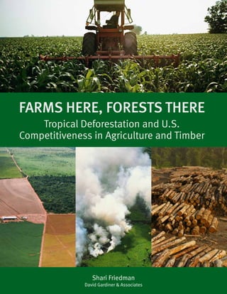
  • 1. Shari Friedman David Gardiner & Associates Farms Here, Forests There Tropical Deforestation and U.S. Competitiveness in Agriculture and Timber
  • 2.
  • 3. i Acknowledgements We greatly appreciate the support of the National Farmers Union and Avoided Deforestation Partners for this report. We are particularly grateful to NFU president Roger Johnson and Jeremy Peters for their thoughtful engagement, and ADP’s Founding Partner Jeff Horowitz and Washington Director Glenn Hurowitz for their contributions. Many different people helped make this report possible. Jonah Busch, Ph.D. of Conservation International and Ruben Lubowski, Ph.D. of the Environmental Defense Fund provided invaluable assistance in the development of the economic models used in the report. Erin Myers Madeira and Andrew Stevenson of Climate Advisers and Resources for the Future gave extensive and important analytic input.The Union of Concerned Scientists provided the resources of its Tropical Forest and Climate Initiative to assist in development and review of the report. Particular thanks go to Douglas Boucher, Ph.D. and Pipa Elias who provided guidance on integration of their own and other groundbreaking research. We are also grateful to the many expert reviewers who provided detailed comments and feedback, including Glenn Bush, Ph.D. of the Woods Hole Research Center, Professor Bruce Babcock at the Center for Agricultural and Rural Development of Iowa State University, Barbara Bramble of the National Wildlife Federation, Sara Brodnax of The Clark Group,Toby Janson-Smith of Conservation International, Professor Brian Murray of Duke University’s Nicholas Institute, Alexia Kelly of the World Resources Institute, Sasha Lyutse of the Natural Resources Defense Council, Anne Pence of Covington and Burling, Annie Petsonk of the Environmental Defense Fund, Nigel Purvis of Climate Advisers, Naomi Swickard of the Voluntary Carbon Standard, Michael Wolosin of The Nature Conservancy and several others. Carley Corda and her team at Glover Park Group designed the report, and special thanks go to Erik Hardenbergh, Ryan Cunningham, and Grant Leslie for their help. Olivier Jarda and Caitlin Werrell provided research support, and Rachel Arends reviewed the design.
  • 4. ii About the Author David Gardiner & Associates prepared the paper on behalf of Avoided Deforestation Partners and the National Farmers Union. Shari Friedman, Senior Advisor to DGA, served as lead author. David Gardiner & Associates helps industry, nonprofits and foundations solve energy and climate challenges. DGA has expertise in climate and energy policy and regulation, as well as tools and strategies for businesses to reduce emissions, lower costs and create advantages within existing or potential policies. DGA also works with foundations and NGOs to develop and pursue strategies that advance their climate and energy goals. Shari Friedman is the President of ASF Associates and Senior Advisor to David Gardiner & Associates. ASF Associates focuses on climate change policy and private sector strategies. Ms. Friedman has 14 years of experience in climate change, including policy development, international negotiations and greenhouse gas markets. She has experience in both the federal government and the private sector. From 1995 to 2001, Ms. Friedman worked on climate change at EPA, analyzing domestic climate change policies and international competitiveness. From 1998 to 2001, Ms. Friedman was part of the U.S. negotiating team for the Kyoto Protocol, focusing on rules for project- level trading, particularly the Clean Development Mechanism. In 2001, Ms. Friedman joined Environmental Enterprises Assistance Fund (EEAF), which managed private equity funds for environmental businesses. Ms. Friedman left EEAF to create Opus4, now ASF Associates. Ms. Friedman has a Masters degree in Public Policy from Georgetown University and a B.A. from Tufts University.
  • 5. iii Contents Executive Summary . . . . . . . . . . . . . . . . . . . . . . . . . . . . . . . . . . . . . . . . . . . . . . . . . . . . . . . . . . . . . . . . . . 1 I. Background . . . . . . . . . . . . . . . . . . . . . . . . . . . . . . . . . . . . . . . . . . . . . . . . . . . . . . . . . . . . . . . . . . . . . . 6 II. Commodity Change Estimates and Impacts on U.S. Markets . . . . . . . . . . . . . . . . . . . . . . . . . . . . 14 a. Soybeans . . . . . . . . . . . . . . . . . . . . . . . . . . . . . . . . . . . . . . . . . . . . . . . . . . . . . . . . . . . . . . . . . 14 b. Vegetable Oil . . . . . . . . . . . . . . . . . . . . . . . . . . . . . . . . . . . . . . . . . . . . . . . . . . . . . . . . . . . . . . 18 c. Beef . . . . . . . . . . . . . . . . . . . . . . . . . . . . . . . . . . . . . . . . . . . . . . . . . . . . . . . . . . . . . . . . . . . . . . 21 d. Timber . . . . . . . . . . . . . . . . . . . . . . . . . . . . . . . . . . . . . . . . . . . . . . . . . . . . . . . . . . . . . . . . . . 24 III. Financial Impact of Tropical Forest Offsets . . . . . . . . . . . . . . . . . . . . . . . . . . . . . . . . . . . . . . . . . . . 28 IV. Conclusion . . . . . . . . . . . . . . . . . . . . . . . . . . . . . . . . . . . . . . . . . . . . . . . . . . . . . . . . . . . . . . . . . . . . . 29
  • 6. iv
  • 7. 1 EXECUTIVE SUMMARY Destruction of the world’s tropical forests by overseas timber, agriculture, and cattle operations has led to a dramatic expansion in production of commodities that compete directly with U.S. products. About 13 million hectares (32 million acres) of forest are destroyed every year — mostly in the tropics.1 This deforestation has allowed large-scale low-cost expansion of timber, cattle and agricultural production, and has also caused damage to the environment and forest communities. Much of this timber and agricultural expansion has come through practices that do not meet U.S. industry standards for sustainability, labor practices, and basic human rights, providing these overseas agricultural operations a competitive advantage over U.S. producers. The U.S. agriculture and forest products industries stand to benefit financially from conservation of tropical forests through climate policy. Ending deforestation through incentives in United States and international climate action would boost U.S. agricultural revenue by an estimated $190 to $270 billion between 2012 and 2030.This increase includes $141 to $221 billion in direct benefits from increased production of soybeans, beef, timber, palm oil and palm oil substitutes, and an estimated $49 billion* savings in the cost of complying with climate regulations due to lower energy and fertilizer costs resulting from the inclusion of relatively low-cost tropical forest offsets. Climate legislation currently under consideration in Congress includes provisions to unlock these benefits for U.S. agriculture through a combination of tropical rainforest offsets and by setting aside allowances for tropical rainforest conservation. Combined with anticipated comparable action by other developed countries, these policies aim to cut tropical deforestation in half by 2020 and eliminate it entirely by 2030. This report analyzes the impact of achieving these conservation goals† on U.S. production of soybeans, palm oil substitutes, beef, and timber. Eliminating deforestation by 2030 will limit revenues for agricultural expansion and logging in tropical countries, * Analysis of the cost of compliance with climate regulation was done by Climate Advisers. See Section III for more details. † These benchmarks are chosen based on global targets for reduced deforestation.
  • 8. 2 providing a more level playing field for U.S. producers in global commodities markets. We examine potential annual effects of a reduction in deforestation as well as the cumulative effect between 2012 and 2030. Methodology This report is a first step in understanding the potential impacts on U.S. agriculture of deforestation and global forest conservation efforts. We consider the impact of reduced production of these commodities on tropical forest lands and estimate how this reduction would affect the world market, taking into account resulting changes in commodity production on non-forest lands in tropical forest nations, the United States, and other parts of the world. We begin by estimating the amount of each commodity that is produced on formerly forested land. We consider the impact of a reduction in the forested land available for agricultural and timber production in the tropics, without considering the underlying government policies and measures that would produce this result. This analysis has been structured around available data and therefore methods are specific to each commodity. Assumptions are outlined in the body of the paper. We use a partial equilibrium model to estimate the impact of this reduction on the world market and the price effects and changes reduced commodity production from deforested land would have for revenue for the U.S. agriculture and timber markets. We use a range of supply and demand elasticities (estimates of the responsiveness of quantity demanded and supplied to changes in price) from existing literature to provide a scope of possible outcomes. In the low revenue scenario, the United States has a limited ability to adjust production in response to market price changes and the rest of the world has a greater ability. In the high revenue scenario, the United States has a greater ability to respond to market price changes and the rest of the world has a more limited ability. We do not consider cross-elasticities or how the price increase of one commodity could affect the revenues of another.This could be a factor for beef revenues if soybean prices increase and vice versa.These factors (discussed more in Annex B) are important to drawing a fuller picture of what would occur under reduced deforestation scenarios. We aim to provide an initial concept of the scope of the issue as a basis to move forward with a fuller analysis. Given time constraints and the dearth of existing data and analysis on this topic, this report makes the best possible use of the resources available. A fuller analysis would incorporate dynamic economic modeling of price changes, estimates of technological improvements, changes in elasticities over time, more disaggregated and detailed country and regional supply reaction and impacts of supply changes in one commodity on production of other commodities.These are recommended areas for further research. Impact of Offsets Allowing international forestry offsets in climate legislation also affects U.S. agriculture and forestry. Because these offsets are among the most affordable means of reducing climate pollution, they would provide significant savings on electricity, fuel, fertilizer, and other input costs for the U.S. agriculture, ranching, Cumulative Revenue Increase to U.S. Agriculture and TImber Producers from Ending Deforestation, 2012 – 2030 Commodity 2008 U.S. $ Billion Soybeans $34.2 – $53.4 Palm Oil and Palm Oil Substitutes (1) $17.8 – $39.9 Beef $52.7 – $67.9 Timber $36.2 – $60.0 Total Cumulative $141.0 – $221.3 (1) Includes crops for soybean oil, cottonseed oil, sunflower oil and canola oil
  • 9. 3 and forest products industries.These input costs are major expenses for the industries analyzed in this report — the agriculture sector alone spends about $10 billion just on energy each year.2 Easing near-term costs of a climate policy allows the sectors to transition more smoothly to carbon-efficient technologies and reduce the overall cost. Allowing capped entities, including energy producers, to “offset” their emissions by investing in affordable emissions reduction options such as tropical forest conservation will reduce permit prices, therefore keeping energy prices low for farmers, ranchers, and the forest products industry.Tropical forest conservation is among the lowest-cost emissions reduction options available, providing important savings for the agriculture and forest products industries. EPA has estimated that the cost of emissions permits in the House-passed American Clean Energy and Security Act would be 89% more expensive if international offsets (the bulk of which are expected to come from tropical forest conservation) were excluded.3 Estimates based on EPA’s analysis of the House-passed American Clean Energy and Security Act indicate that the inclusion of international offsets will save the agriculture, forestry, fishing and timber industries about $4.6 billion per year and $89 billion between 2012 and 2030.4 With tropical forest conservation likely to comprise an estimated 56% of offsets in the years immediately following implementation of climate legislation (though more afterwards), this translates into a cost savings for these industries of approximately $49 billion between 2012 and 20305 (see Section III).
  • 10. 4 T his paper focuses on the economic impacts of deforestation — and forest conservation — on the U.S. agriculture and timber industries. But what about the impact on people in the rainforest nations themselves? Right now, many people in rainforest nations face a terrible choice. In the absence of incentives for their protection, forests are worth more dead than alive. A company or peasant is forced to weigh the very immediate financial proceeds of cutting down a forest for timber, agriculture, or ranching against the damage wrought by deforestation to their own communities, wildlife, water and the planet — as well as the lost potential future financial value of the land as a carbon sink. Even if clearing and burning a hectare of rainforest only produces ranchland worth $200 per hectare, many people make the choice to cut it down anyway — because that deforestation can, at least in the short run, put food on the table or boost earnings for a quarterly report to investors. But that decision comes at a terrible long-term economic price. Based on recent prices in European carbon markets, the value of a hectare of rainforest as a carbon sink is approximately $10,000 a hectare. Releasing that carbon into the atmosphere by clearing or burning the forest means sacrificing the opportunity to realize that value. As a recent World Bank report put it, “Farmers are destroying a $10,000 asset to create one worth $200.” * So how will providing financial incentives for the conservation of forests affect those who are profiting from deforestation? In most cases, the people cutting down the forests have the most to gain from conserving forests. Because incentives to end deforestation are established to, in part, compensate those who lose money by bypassing an opportunity to deforest, the farmers, loggers, and landowners themselves tend to have the most to gain.They will be the ones compensated — they can gain income far exceeding SIDEBAR: The Impact of Deforestation on People in Rainforest Nations any profits from deforestation, and enjoy enormous benefits to their local communities and environments. For instance, in Brazil, many of the ranchers and farmers most responsible for deforestation have become advocates of forest conservation programs. Pilot projects and an increasing recognition of the high costs of deforestation have convinced many that they and their communities will become richer — and also enjoy a better quality of life — through conserving forests rather than cutting them down. Perhaps the most prominent embodiment of these new conservationists is Blairo Maggi, Brazil’s “King of Soy” — the country’s biggest private landowner, personally responsible for tens of thousands of acres of forest destruction, and governor of Mato Grosso province, ground zero for deforestation. Maggi made his name throughout the world as an enemy of conservationists and a vocal ideological defender of deforestation as the path to riches for himself and the citizens of his state. Maggi has changed, however. He has recently urged adoption of policies to conserve the forest — if the state can find developed country governments or private companies who will finance forest conservation, most likely as part of a mandatory carbon reduction system. Forest conservation incentives “will be much, much more profitable than soybeans,” he told Forbes Magazine.† In addition, even a small carbon incentive can do a lot to bring production in rainforest nations up to the environmental and social standards of the United States and other developed countries. Protecting forests will also create much needed, well-paying jobs in developing countries. Forest conservation requires people: park rangers to patrol the forest, foresters to measure carbon storage, and even satellite manufacturers and operators to provide deforestation monitoring. Reforestation activities * Chomitz, Kenneth. At Loggerheads? Washington, DC: The World Bank, 2007. † Perlroth, Nicole. “Tree Hugger.” Forbes Asia Magazine. December 14, 2009. http://www.forbes.com/global/2009/1214/issues-blairo-maggi- jungle-conservation-tree-hugger.html
  • 11. 5 that often accompany forest conservation can provide additional employment opportunities. Protecting existing forests will also provide a more sustainable source of jobs in extractive industries themselves. In places without conservation incentives, forests are routinely stripped of all their value and the ground is left as a barren desert that can’t support communities or jobs. For this reason, many producers in tropical countries have advocated establishing carbon incentives that would rapidly shift production to more sustainable sources. In Indonesia, for example, clear cutting has drastically reduced the availability of trees to provide employment in forestry, including logging. According to the Indonesian forestry union, Kahutindo, employment in forest products has declined by more than 50 percent in the past decade, from 2 million workers to fewer than 1 million today. As a result, Kahutindo now advocates conserving existing rainforests and relying solely on reforestation to produce fiber. ** There is evidence that this strategy will work globally to create well-paying jobs in the forestry sector. The latest U.N. Food and Agriculture Organization State of the Forests report estimated that switching to sustainable forest management would create 10 million good jobs globally, which would create a major force against rural unemployment, underemployment and poverty.†† Benefits in the agricultural and ranching sectors are likely to be significantly greater, given the greater economic values. Providing financial incentives for forest preservation will allow a wide array of people, from peasants to landowners, to preserve the forests we all need to fight climate change. – Glenn Hurowitz ** Foster, David. “Indonesia’s Forestry Workers – Another Endangered Species.” December 11, 2007. http://blog.aflcio. org/2007/12/11/indonesias-forestry-workersanother-endangered-species/ †† Food and Agriculture Organization of the United Nations. “Forests and the global economy” March 10, 2009. http:// www.fao.org/news/story/en/item/10442/icode/
  • 12. 6 I. BACKGROUND Tropical rainforests store an immense amount of carbon. Clearing and burning these forests releases this carbon into the atmosphere in the form of carbon dioxide. An estimated 15% or more of total global carbon dioxide emissions comes from tropical deforestation.6 Indonesia and Brazil, for example, rank as the third and four largest emitters, respectively, almost entirely due to deforestation.7 Despite the immense amounts of carbon stored in tropical forests — deforestation releases an average of about 500 tons of carbon dioxide per hectare — incentives for their conservation were excluded from the Kyoto Protocol and most other major climate policies. Without these conservation incentives, deforestation continues to occur at a rapid rate, much of it due to logging and conversion of forestland to agricultural uses. Deforestation occurs mainly because other land uses in many cases generate greater immediate financial returns than retaining the land as forest.8 Alternate uses putting pressure on forests include croplands, pastures and plantations.9 Today, an acre of natural tropical forest holds potential monetary value from the extracted wood and subsequent commodities grown or raised on the land, but holds little financial potential as a natural forest. Although subsistence activities have dominated agricultural-driven tropical deforestation, large-scale commercial activities are playing an increasingly significant role, particularly in the Amazon, Indonesia and Malaysia.10 Globally, foreign commercial agriculture and timber production have become the leading cause of deforestation. Without policies that create value for the environmental services that forests provide, tropical forests are often worth more money dead than alive. Foreign agricultural, logging and ranching operations are able to take advantage of cheap land supply and undercut U.S. producers on the world market. The main agricultural commodities that drive tropical deforestation today include soybeans, palm oil and cattle. Soybean cultivation and cattle are drivers of deforestation in Brazil and soy also contributes to deforestation in Argentina. Palm oil is a major cause of deforestation in Indonesia and Malaysia.11 The expansion of pasture and plantation to previously forested land in nations such as Brazil, Argentina, Indonesia and Malaysia has contributed to these countries becoming lead producers and exporters of these commodities.
  • 13. 7 If the forests are conserved, the land will not be converted to pasture or plantation. While some production will be shifted to other land in the country or yield per acre may increase more than it would have without pressure from land restrictions, we can expect to see reduced production from these countries as a result of restricted land and higher production costs.* In addition, forests will remain intact, reducing the influx of timber products into the international market. The degree to which each country would be able to intensify production in response to the restricted supply of cheap agricultural land from forested areas would depend on each country’s land base and economic conditions that determine how much it is likely to expand cropland and yields on existing agricultural land or on other available non-forest land. The ability of one country to capture market share is a function of its own supply possibilities as well as those of other countries.† Further, a restriction in supply will likely have price impacts that then affect demand levels and also production choices. The interaction among crops and also between crops, pastureland, plantations and intact forests is dependent on many variables, including the prices of each commodity — whether a crop, timber or the value of a standing forest. A further consideration is that soy is a key feed ingredient for cattle, causing a relationship between price increases for soy and production of beef. Economists are beginning to develop models specifically designed to examine the effect of different bioenergy and climate policies on global agricultural and forestry production and prices. One recent study just published in November 2009 by Alla Golub of Purdue University and coauthors finds results consistent with this report. The Golub study uses a general equilibrium model that links global agriculture and forestry to look at how different land use opportunities for greenhouse gas abatement interact with each other. The study finds that a $100/ ton carbon price leads to an expansion over business as usual of standing tropical forests that reduces the amount of land available for crops and grazing. The paper finds that this reduction in available land, among other factors, leads to agricultural and cattle production shifting to other countries. Under the $100/ton carbon price, their model estimates that the United States increases its crop production from between one and four percent and its cattle production by two percent.12 An Iowa State University study by Kanlaya J. Barr and coauthors estimates elasticities of land supply for agricultural commodities in the United States and Brazil, both major producers and exporters of soybeans and beef. These elasticities capture the willingness of producers in each country to transform land from one use to another. In this case, it analyzes likely choices between forest, crops and pasture. The paper focuses on the effect that agriculture price increases would have on land choices.They estimate that cropland elasticities in the United States are much lower than those of Brazil.13 In a related study, Michael J. Roberts and Wolfram Schlenker seek to understand how global food price and quantities supplied vary with respect to changes in supply due to biofuel demand and other factors.Their report finds that major producers and exporters, such as the United States and Brazil, demonstrate higher elasticities of supply in relation to producers that consume most of their own output.14 Also, they find higher elasticities of supply for the United States than found by Barr. Blandine Antoine et al. also examine land use changes in forested areas, considering recreational value in addition to crops, pastures, managed forests and national forests. The Antoine study uses elasticities of land transformation that are similar to those used in Golub et al.15 Although these studies provide a basis for further understanding of the impact of reduced deforestation on various markets, there has not been any published analysis of the effect of deforestation alone on the * Production costs are higher because the least-cost option (deforestation) is no longer available. † Gan et al. finds that in the forestry sector, shifting to sustainable harvest will increase production costs and therefore shift some of the production from one country to another.
  • 14. 8 U.S. agriculture and timber markets. An integrated economic model would best address the complicated interactions of price and supply between and among these sectors. Individual commodity models used within the industry will also provide useful results. In the immediate absence of such models, we seek to provide an initial indication of the magnitude of impact that a reduction in deforestation could have on selected sectors. Estimating restricted commodity supply. While data on these commodities is plentiful, most data include crops from plantations and existing yields. We seek to estimate the effect of a reduction in deforestation only and therefore have developed individual methods based on deforestation rates, yield and other relevant data.* Not all deforestation results in greater supplies of timber or agricultural commodities to the global market. Wood from tropical forests may also be used as fuel wood in local markets, destroyed as collateral damage to create roads, burned, or decomposed. Once cleared, land can be used for industrial purposes, roads, development, or tree farming as well as agriculture. Since no global estimates exist for the amount of deforestation driven by different commodities, we identified the main countries where the commodity was a driver of deforestation and considered only those countries in the analysis. We first gathered data from articles and published research that analyzed the degree to which particular commodities drive deforestation in different places. We then excluded those countries without high deforestation rates in order to focus only on those places where commodity expansion is driving deforestation. Because of the lack of global data, we estimate production shifts from the countries where the production of a given commodity is a significant driver of deforestation. Because we are only looking at a sample of countries, we risk missing some shifts in commodity production that are likely to result from forest conservation. For some commodities, such as beef, this is likely a minor issue since deforestation for commercial beef production is predominantly in Brazil. For timber, however, our focus on a subset of countries likely leads to underestimating the impact since more countries than the five we examine harvest tropical forests and sell the timber in international markets. We use existing data and simple calculations to estimate the amount of a commodity that is grown Intro Table 1: Tropical Deforestation — Top 20 Countries (3) Country (1) Annual Deforestation Rate (hectares) (2) Brazil 3,103,000 Indonesia 1,871,000 Sudan 589,000 Myanmar 466,000 Zambia 445,000 Tanzania 412,000 Nigeria 410,000 DR Congo 319,000 Zimbabwe 313,000 Bolivia 270,000 Mexico 260,000 Venezuela 228,000 Cameroon 220,000 Cambodia 219,000 Ecuador 198,000 Australia 193,000 Paraguay 179,000 Philippines 157,000 Honduras 156,000 Argentina 150,000 (1) Country list compiled from NASA Earth Observatory, Tropical Deforestation: causes of deforestation, http://earthobservatory. nasa.gov/Features/Deforestation/deforestation_update3.php. February 1, 2010 (2) Food and Agricultural Organization of the United Nations, “State of the World’s Forests”, 2009. Average annual change rate in forest cover 2000 – 2005. (3) Annual change rate does not directly correlate to emissions, as deforestation listed above includes both dry and tropical forests. * Methods vary by commodity depending on available data and market circumstances.
  • 15. 9 on or extracted for sale from formerly forested land. Data on this topic is sparse. We were not able to find one data set that could be used for all the sectors. As a result, we developed individual methods to estimate the production of each commodity on deforested land. These methods are described in the subsections below. Estimating the impact on the U.S. markets for each commodity. We combine our estimated avoided tropical production with a partial equilibrium model, based on current commodity prices and estimates of supply and demand elasticities.The model is geographically divided into tropical forest countries (those where agricultural and timber production are the lead drivers of deforestation), the United States and the Rest of the World (ROW). The elasticities represent a range found in existing literature. Demand elasticities indicate the amount of a commodity that the market will purchase given a change in the price. The higher the elasticity, the more consumers will react to a price change by, for example, switching to substitute products. For each commodity, we used a single global elasticity of demand, since these are globally traded commodities. We averaged the high and low elasticities of demand to define a linear global demand curve. For agricultural commodities (including beef), we used data from the FAPRI elasticity database.16 For timber, we used demand elasticities from Waggener and Lane (1997).17 Elasticities of demand will likely change over different price ranges as well as over time as global consumption patterns change. These elasticities will also vary according to different time horizons as consumers will have greater ability to adjust diets and find substitutes over longer periods. We use current estimates and do
  • 16. 10 not attempt to account for future changes in demand. Supply elasticities represent the change in the amount of a commodity that producers will supply given a change in price.These incorporate a country’s ability to increase yield rates, land availability and capital constraints. For each commodity examined, we use the estimated supply elasticities to define a set of three linear supply curves for the United States, rainforest nations, and the rest of the world. We estimated a high and low supply elasticity to provide a range. We drew heavily from the FAPRI database, but also used commodity-specific elasticities where appropriate (see Annex D for further discussion of elasticity choices). In general, the supply elasticities used in this analysis are short-term to mid-term. One might expect that longer- term supply elasticities would be higher as they would incorporate greater adjustments in production. The combination of our estimated supply and demand curves indicates the global price equilibrium of a commodity and how much each country is likely to supply at that price (see Annex C for further discussion). It’s important to note that the estimated decrease in supply or supply growth and increase in prices reported in this paper represent changes only for the individual commodity and are not reflective of food supply or prices in general. In world food markets, commodities are substituted and technologies are constantly evolving, affecting net food supply and price. To understand the range of possible impacts on individual commodity producers in the United States, we use both high and low estimates of changes to U.S. revenue. High U.S. revenue estimates are based on high elasticities of supply for the U.S. and low elasticities of supply for rainforest nations and ROW. In other words, under this scenario, the United States is more likely to adjust production in response to price increases and production gaps than the rest of the world. Our low U.S. revenue estimates are based on high elasticities of supply for rainforest nations and ROW and low supply elasticities for the United States where the United States is relatively less likely to change production given price increases and production gaps than the rest of the world. Using one elasticity of supply for rainforest nations and ROW does not account for individual countries’ abilities to react to the market. For example, in timber markets, northern European timber output has been declining due to reduced harvesting, as it is not price competitive. However, productive capacity exists and Europe may have an ability to respond fairly quickly to fill a shortfall in world market supply of lumber. This specific elasticity is aggregated into the ROW estimate. Although less detailed, this estimate provides a more simple and transparent analysis for this preliminary study. The partial equilibrium model provides estimates of annual price effects and production/revenue effects of decreasing production on forested land. Results show the increase in revenue to U.S. agriculture and timber from both a price increase and also an increase in production.The analysis does not differentiate between the change in production due to land expansion versus an increase in yield.These effects are in principle captured in the elasticities of supply for each commodity and region, which would have a different set of opportunities to increase production. Under a system of protected forests, rainforest nations are still likely to have opportunities for agricultural expansion into non-forested land or reforestation for timber production. As noted above, while the partial equilibrium model accounts for how each country or region will behave with a price increase of a given commodity, it does not consider the interactions between commodities. Estimating cumulative impacts. Once a plantation or grazing area is established, the yield enters the market in subsequent years. However, deforested land’s poor fertility combined with poor agricultural practices can cause land, particularly that used for cattle ranching, to decline in productivity. As a result, ranchers often abandon their land after just a few years and clear additional forest to accommodate their herd.This abandon-and-deforest process adds significantly to the deforestation produced by certain commodities,
  • 17. 11 particularly cattle. Cumulative estimates for each commodity included in this paper are based on estimates of that commodity’s likelihood to continue production on cleared land. For soybeans and oilseeds, we assume that the cleared land will produce each year between 2012 and 2030. For cattle, we assume it will produce for five years and then cease to be productive pasture land (see Section II.c for more detail). Timber is harvested once and assumed not to regenerate for commercial timber production within the timeframes considered in this study. We used the partial equilibrium model to estimate the cumulative revenue increase for each commodity of a gradual reduction in deforestation from 0 to 100% between 2012 and 2030, hitting a 50% reduction in deforestation at 2020. We include several simplified assumptions. We measure the impact of reducing deforestation relative to a stylized scenario where future production only increases as a result of estimated tropical deforestation. We also assume this production increase at the forest frontier exactly satisfies future demand growth so that prices stay constant in real (inflation adjusted) terms. Additionally, we assume the estimated supply and demand elasticities stay constant over time.This simple baseline scenario ignores trends in yield growth and other factors and is intended to provide a simple indication of the potential magnitudes of the effects. In addition, the model does not adjust for short-term and long-term elasticities. In the long run, sustained price increases influence a variety of market adjustments that shift demand and supply.This would lead to higher long-run elasticities of both supply and demand, which are not estimated in our model.The model therefore allows for long-term sustained price increases, which lead to higher prices in the later years than one would expect over the long run. Using these assumptions and inputs, we used the partial equilibrium model to estimate the amount of reduced tropical production that the United States would supply and the additional revenue due to associated price increases. State-level impacts. For each commodity, the cumulative impacts are broken down by state, based on existing production. We calculate the percentage that each state producers based on USDA and Census data and ascribe the increased production value to each state based on this data. Past production is an imperfect proxy for future expansion, as it does not consider state- specific factors such as land availability restrictions or opportunity costs of other crops. We present it here as a rough distribution indication, acknowledging that the aforementioned factors could shift how an increase in U.S. supply would be met. Subsequent analysis should more thoroughly consider state-specific elasticities of supply.
  • 18. 12 O ne of the most contentious areas of energy and climate policy has been a major dispute about whether or not biofuels produced or consumed in the United States and other developed countries are driving deforestation. A number of studies published in prominent scientific journals have concluded that growing crops for fuel in the United States and Europe displaces food crops, leading to higher food prices and greater demand for agricultural products that in turn drives deforestation for agricultural expansion.* As a result of this “indirect land use” impact, these studies found that ethanol and other biofuels caused significantly more climate pollution than the gasoline they are meant to replace. In a report published in the journal Science, for instance, Princeton University’s Tim Searchinger found that corn-based ethanol grown in the United States increased greenhouse gas emissions for 167 years over gasoline.† SIDEBAR: Ending the Ethanol Wars Biofuels manufactuers, growers and others have disputed these findings, arguing that land use decisions in tropical countries are driven by many forces other than developed country energy and land use policy — and that increasing yields from many crops could counteract any indirect land use impacts.** There’s a lot at stake in this debate — and not just for the environment.The 2007 Energy Independence and Security Act mandated the production of 36 billion gallons of biofuels by 2022 (a quadrupling of current production), but required 22.3 billion gallons of that to be subject to lifecycle greenhouse gas analysis to ensure that it actually reduced pollution relative to gasoline. As part of that analysis, it stipulated that indirect land use impacts such as tropical deforestation be used to calculate the total greenhouse gas impact of biofuels.†† If ethanol is found to indeed drive deforestation at significant levels, it would be ineligible to fill the demand created by part of the 36 billion gallon mandate — significantly reducing a source of income for corn growers and ethanol manufacturers. Although stark disagreements about the environmental impact of ethanol persist, environmentalists and biofuels producers have reached a consensus that protecting rainforests through climate finance mechanisms will dramatically reduce any indirect land use concerns. In most parts of the world, even additional income from biofuels can’t come close to generating the levels of revenue that could be available to landowners from climate finance incentives for forest conservation — meaning that tropical forests will generally stay intact. As a result, protecting rainforests through climate finance will allow biofuels producers and growers in the United States to prosper with fewer concerns about the environmental impact of their production. “REDD can help reduce the potential for any direct and indirect effects of bioenergy production on greenhouse gas emissions from changes in agriculture and other land uses.” —Annie Petsonk Environmental Defense Fund * Fargione, Joseph; Jason Hill, David Tilman; Stephen Polansky; and Peter Hawthorne. “Land Clearing and the Biofuel Carbon Debt,” Science. Vol. 319, No. 29. February 29, 2008. P. 1235-1238. † Searchinger,Timothy; Ralph Heimlich; R.A. Houghton; Amani Elobeid; Jacinto Fabiosa; Simla Tokgoz; Dermot Hayes; and Tun-Hsiang Yu. “Use of U.S. Croplands for Biofuels Increases Greenhouse Gases Through Emissions from Land Use Change.” Science. February 29, 2008. Vol 319, no. 5867. P. 1238-1240. ** Khosla, Vinod. “Biofuels: Clarifying Assumptions.” Science. Vol. 322, No. 5900. October 17, 2008. P. 371-374. †† Energy Independence and Security Act,Title II
  • 19. 13 “The Ohio Corn Growers Association recognizes that the indirect land use debate has many arguments on both sides of the issue. Regardless, stopping tropical deforestation is a win for U.S. agriculture’s competitiveness as well as ending the debate on corn’s role in indirect land use.” —Dwayne Siekman Ohio Corn Growers Association
  • 20. 14 a. Soybeans The United States is the leading producer of soybeans with 33% of global production in 2007, followed by Brazil, Argentina, and China.18 The United States is also the top exporter of soybeans, accounting for 40% of global exports in 2007, followed by Brazil, Argentina, Paraguay and Canada. The relationship between soy cultivation and deforestation in the Amazon is complex. In 2003, soybeans accounted for approximately four percent of the agricultural land in the Amazon. Most Amazon soybeans are grown on large-scale commercial plantations.19 In some instances, commercial soy cultivation is not an initial driver, but follows initial deforestation for other purposes. Cattle ranchers or small-scale farmers deforest the land and then move on when the soil has become depleted. Commercial soy operations recondition the land and create long-term soy plantations.19 Increasingly, however, large-scale agriculture itself is the primary driver of deforestation. A National Academies of Science study of Brazil’s Mato Grosso state by Morton et al. shows that 17% of deforestation was caused by large-scale agriculture between 2001 and 2004. Further, this expansion closely tracks global soybean prices — as prices go up, more land is cleared for large-scale agriculture.20 The increase in soybean cultivation as a driver of deforestation is partially due to expanded transportation infrastructure in forested regions. Production of soybeans in closed-canopy forest increased 15% per year from 1999 to 2004.21 The price of forested land is substantially cheaper than other agricultural land in Brazil. In 2004, uncleared Brazilian savannah or forest cost about US$50/acre. In contrast, cleared Brazilian agricultural land ranged in price between $100 and $300.22 Whether commercial soy plantations are the driver or the secondary beneficiary, unprotected forests are leading to expanded soy cultivation in the tropics. Argentina has also emerged as a leader in soy production and exports. In Argentina, expansion in soybeans has replaced other crops. However, the introduction of new soy varieties and other factors have led to deforestation for soy plantations.23 Together, the United States, Brazil and Argentina produce about four-fifths of the world’s soybean crop and account for 90% of global exports.24 Recent studies suggest that soybean production in Brazil and Argentina affects world markets, including those in the United States. A USDA analysis found that exports from Brazil and Argentina were projected to cause a reduction in U.S. soybean exports.25 Additional data show that the United States is able to pick up gaps in global production. In the 2008 – 2009 growing season, global soybean production decreased by 11%. In response, the United States increased production, pulling the world soybean output up by five percent, counteracting the sharp declines in production in Argentina, Brazil and Paraguay.26 Table SB1: Global Soybean Producers, 2007 Country Production (tonnes) % World Production United States 72,860,400 33% Brazil 57,857,200 26% Argentina 47,482,784 22% China 13,800,147 6% Source: Food and Agricultural Organization of the United Nations, FAOStat, FAO Statistics Division (2009) Table SB2: Top Global Soybean Exporters, 2007 Country Export Quantity (tonnes) % World Exports United States 29,840,182 40% Brazil 23,733,776 32% Argentina 11,842,537 16% Paraguay 3,520,813 5% Source: Food and Agriculture Organization of the United Nations, FAOStat, FAO Statistics Division (2009) II. COMMODITY CHANGE ESTIMATES AND IMPACTS ON U.S. MARKETS
  • 21. 15 To get a preliminary understanding of how deforestation affects soy producers in the United States, we examined the amount of soybeans entering the market on land that was cleared for soybean growth in Argentina, Brazil and Paraguay.This does not include soybean production on land that was cleared for other purposes and then converted to soy plantations. Total deforestation for these countries combined is 3.4 million hectares (3.1 million in Brazil, 0.18 million in Paraguay and 0.15 million in Argentina*).27 Given the lack of conclusive data on the drivers of deforestation, we extrapolated the information reported in Morton’s study and assumed that 17% of the deforestation in each country was due to large-scale agriculture.28 In the literature reviewed for this study, soy was the prime (and often only) commodity discussed for large-scale commercial crops in the Amazon. Nonetheless, we assumed that it is reasonable that some other large-scale crops are growing on this land and conservatively discounted our estimate by 20% to account for potential attribution errors for other crops.† Given a yield of 2.97, 2.81, and 2.41 tonnes per hectare for Argentina, Brazil and Paraguay respectively,29 we estimate the annual avoided expanded production from the forest frontier at 653,000 tonnes per year if deforestation is halved and approximately 1,306,500 tonnes per year if net deforestation is eliminated entirely. Using a partial equilibrium model, we estimated the effect on U.S. soybean revenue that would result from reduced deforestation in Brazil, Argentina and Paraguay. We used a 2008 price of $323/tonne.30 * Numbers are rounded to the nearest thousand. † Most literature on this topic addresses soy as the large-scale agricultural crop.The study noted above by D.C. Morton et al. notes that deforesta- tion for large-scale crops in Mato Grosso is highly correlated with global soy prices, indicating that soy is a main driver. In the absence of data indicating other crops driving large-scale agriculture in the Amazon, we assume 20% as a proxy and apply a discount factor of 0.8.
  • 22. 16 Table SB3 shows the annual production data used.The first row of Table SB3 shows our estimate of the annual amount of soybeans that is grown on rainforests cleared for soybean cultivation (based on our analysis described above).The second row shows all the soybeans that enter the market from Brazil, Argentina and Paraguay. These two rows are different because not all soybeans from these countries are grown on land deforested for soybean cultivation. Some is grown on land other than tropical forest and some is grown on land that was forested, but was cleared for reasons other than soybeans. It’s common that land is cleared for livestock grazing, but then converted to soy plantations. In some cases, the baseline production in these countries is from land that was cleared for soybean production in previous years and now enters the market annually. To estimate supply response, we use the average soybean-specific demand elasticity of -0.275.31 This means that the global demand for soybeans declines by about 0.275% for each 1% increase in the price of soybeans.To estimate supply response, we use a high supply elasticity of 0.2532 and a low supply elasticity of 0.633 for the three regions evaluated in the model (tropical forest countries, the United State and the rest of the world). While elasticities of supply are likely to differ between the regions, these elasticities represent an approximate middle-range within available literature.This mid-range allows us to examine what could happen if the U.S. has a relatively higher ability to react than the rest of the world and vice versa. In the long run, we would expect supply elasticities to be higher, accounting for various market adjustments that affect supply. Individual suppliers face more long-run options such as technology shifts or shifts to other production sources (in this case, other types of land). Long-term global supply can also shift because new entrants are likely to enter the market if prices are higher, or exit the market if prices are lower.Therefore, the price effects in the later years are likely smaller than our model estimates. (See Annex D for further discussion of the partial equilibrium model and data inputs.) We used two scenarios with different elasticities of supply to represent the likely high and low impact on U.S. revenue.These scenarios were: (1) high supply elasticity for the United States and low supply elasticity for rainforest nations and the rest of the world; and (2) low supply elasticity for the United States and high supply elasticity for rainforest nations and the rest of the world. For each scenario, we estimated the annual impacts at both a 50% and 100% reduction in deforestation.Table SB4 shows the results. All results are reported in 2008 U.S. dollars. Where the U.S. has a higher ability to react to price increases, annual U.S. revenue increases by $590 million if deforestation is ended. Where U.S. ability to react to price is less than the rest of the world, annual U.S. revenue increases by $387 million with zero deforestation. The cumulative effects assume that a 100% reduction in deforestation is achieved gradually with 10% in 2012 increasing annually to 100% in 2030. We assume that once the land is cleared for soybean cultivation, the crop will continue to produce from 2012 to 2030. For simplicity, we assume that increases in production from deforestation are exactly enough to meet future increases in demand such that real prices stay Table SB3: Annual Soybean Production by Region, 2007 Country/Region Tonnes Annual soybean production that drives deforestation (1) 1,306,534 Other annual soybean production from Brazil, Argentina and Paraguay (2) 109,889,450 United States 72,860,400 Rest of World 36,476,228 Source: Food and Agriculture Organization of the United Nations, FAOStat, FAO Statistics Division (1) Calculated from methods described above (2) equals [Total production from Brazil, Argentina, and Paraguay as reported by FAO] — [Annual soybean production that drives deforestation]
  • 23. 17 constant over time. Future sources of demand, such as population growth, changing diets in developing countries, and growing biofuel use could increase the price more than is reflected in our model, while yield growth and other sources of supply outside the tropics could lead to lower prices. In the cumulative analysis, the model shows price increases each year, which are initially less than the annual price increase and become higher than the annual percentage change in later years. This is because the amount of soybeans not entering the market in early years are added to those not entering the market in later years. In year one, the price (in 2008 dollars) is estimated to increase by between $2 and $3 per tonne (a 0.6% to 0.9% increase over 2008 prices). In year 19, the price increases between $51 and $60 per tonne (a 15.8 % to 18.6% increase over 2008 prices). Long-run elasticities that allow for market adjustments would reduce the price effects especially in later years. Given these assumptions, the cumulative increase in revenue to U.S. soybean growers from 2012 to 2030 with gradual forest protection up to 100% in 2030 would be between $34.2 billion and $53.4 billion. Soy production in the United States is concentrated in the South and Midwest, with some production on the East Coast.Table SB5 shows how much revenue each U.S. state stands to gain from gradually eliminating deforestation, presuming proportional benefits to different states based on current production levels.The high and low estimates are based on the cumulative estimates between 2012 and 2030 that are described above. Annex E shows projected revenue increases for all states. Table SB4: Soybean Modeling Results Scenario Price Change (Annual) Annual U.S. Revenue Increase Cumulative Revenue Increase to U.S. from Ending Deforestation, 2012 – 2030$/tonne % Change U.S.$ % Change Low U.S. Revenue 50% reduction in deforestation $3 1.03% $265,384,316 1.13% $34,198,100,533 100% reduction in deforestation $4.67 1.45% $386,824,566 1.64% High U.S. Revenue 50% reduction in deforestation $4 1.20% $405,005,077 1.72% $53,441,145,875 100% reduction in deforestation $5.49 1.70% $590,833,044 2.51% Table SB5: State-level Soybean Revenue Increases From Rainforest Conservation State (1) Cumulative Revenue Increase from Ending Deforestation, 2012 – 2030 (Range in millions) Iowa $4,945 – $7,728 Illinois $4,376 – $6,839 Minnesota $2,898 – $4,528 Indiana $2,712 – $4,238 Nebraska $2,640 – $4,125 Missouri $2,346 – $3,666 Ohio $2,259 – $3,529 South Dakota $1,791 – $2,798 Kansas $1,634 – $2,554 Arkansas $1,248 – $1,950 (1) State rank from USDA, National Agricultural Statistics Service. Based on 2009 production data.
  • 24. 18 b. Vegetable Oil The greatest driver of deforestation in Asia is palm oil cultivation.34 Rubber, sugarcane and coffee also contribute, but to a much lesser extent.35 The growth in palm oil production is largely a result of growing demand for food, cosmetics and biofuels.36 Seventy- seven percent of palm oil is used for food,37 but demand as a fuel source has risen, especially in Europe.38 Indonesia and Malaysia are the major producers of palm oil and related products, together accounting for about 88% of total world palm oil production.39 Over half the new oil palm plantations between 1990 and 2005 in Indonesia and Malaysia were established on newly deforested land. This is partly because logging generates revenue that covers initial costs of establishing the plantation.40 Palm oil directly competes with — and is easily replaced by — other oils including canola (rapeseed) oil, sunflower oil, cottonseed oil, and soybean oil.41 Most products containing palm oil, palm kernel oil, or derivatives such as palmitate frequently exchange these other edible oils depending on small variations in price and availability. While the United States does not produce any palm fruit, it ranks fourth in production of the other oilseeds noted above. Since some crops have other uses (e.g., only 19% of soybeans are used for oil), we calculated the amount used for oil. Table PO1 shows the top producers of
  • 25. 19 oilseeds (palm fruit, rapeseed (canola), sunflower seed, cottonseed and soybeans*). Indonesia and Malaysia collectively produced more than 152 million tonnes of palm fruit and 32† million tonnes of palm oil in 2007, of which over 22 million tonnes were exported.42 Their combined average annual production increase of palm fruit between 2000 and 2007 was over 9 million tonnes — more than 5.9 million tonnes in Indonesia and 3.2 million tonnes in Malaysia.43 The percentage of palm production in Indonesia and Malaysia associated with deforestation is 57% and 56% respectively.44 Given existing yields and market conditions, we estimate that ending deforestation would reduce business as usual supply of palm fruit by 5 million tonnes. Using the partial equilibrium model, we estimated the effect on U.S. oilseed producers that would result from reduced deforestation in Indonesia and Malaysia. Table PO2 shows the annual production data.The first row of Table PO2 shows our estimate of the annual amount of palm production grown on land cleared for palm plantations (based on our analysis described above).The second row shows the remainder of palm and oilseed production that enters the market from Indonesia and Malaysia.These numbers are different because not all palm production from these countries comes from land deforested for palm plantations. Some is grown in other areas of the country and some is grown on land that was formerly forested, but was not deforested that year for palm production. We input the above information into our partial equilibrium model, using the average oilseed-specific demand elasticity of -0.305 and a mix of high and low global oilseed supply elasticities of 0.2545 to 0.6.46 These are the same supply elasticities used in the soybean analysis and provide a simple, transparent method.These high and low elasticities of supply are alternated between regions depending on the scenario (i.e., high U.S. revenue or low U.S. revenue scenario). Aggregating high and low elasticities of supply for all regions does not allow for individual country estimates. However, these serve as approximate numbers that lie within the upper and lower boundaries of the supply elasticities that we found in existing literature. In the long run, we would expect supply elasticities to be higher, accounting for various market adjustments that affect supply (see section II.a for further discussion). For the price in a business as usual scenario, we used * The soybean market will be affected by tropical forested countries decreasing both soybean and palm oil production. When analyzing soybean supply as a substitute for palm oil, we only count the amount of U.S. soybean production that is historically allocated to make soybean oil. † Numbers are rounded to the nearest 0.1 million Table PO1: Top Global Producers of Palm Oil and Palm Oil Substitutes, 2007 (1) Country Production Quantity (Tonnes) (2) % Global Production Malaysia 79,100,000 24.63% Indonesia 78,117,784 24.32% China 18,440,572 5.74% United States 17,383,302 5.41% India 12,991,650 4.04% Brazil 12,549,340 3.91% Source: Food and Agricultural Organization of the United Nations, FAOStats, FAO Statistics Division (1) Palm oil substitutes include cottonseed oil, canola oil, soybean oil and sunflower oil (2) Oilseed production is discounted for the percentage generally used for oil versus other uses. Percentage of each oilseed used for oil are assumed to be: palm fruit — 100%; rapeseed (canola) — 100%; cotton seed — 16.2%; soybeans — 19%; sunflower seeds — 91%. PO2: Annual Oilseed Production by Region, 2007 Country/Region Tonnes Annual palm and oilseed production that drives deforestation (1) 5,161,743 Other annual palm and oilseed production from Indonesia and Malaysia (2) 152,056,042 Annual U.S. oilseed production 17,383,302 Annual Rest of World oilseed production 146,589,556 Source: Food and Agriculture Organization of the United Nations, FAOStat, FAO Statistics Division (1) Calculated from methods described above (2) equals [Total production from Indonesia and Malaysia as reported by FAO] — [Annual palm production that drives deforestation]
  • 26. 20 an average 2008 price of oilseeds (weighted by U.S. production) of $324/tonne.47 (See Annex D for further discussion of the partial equilibrium model and data inputs.) We used two scenarios with different elasticities of supply to represent the likely high and low impact on U.S. revenue. These scenarios were: (1) high supply elasticity for the U.S and low supply elasticity for rainforest nations and the rest of the world (which represents the high revenue estimate); and (2) low supply elasticity for the United States and high supply elasticity for rainforest nations and the rest of the world (which provides the low revenue estimate). For each scenario, we estimated the annual impacts at both a 50% and 100% reduction in deforestation. Table PO3 shows the results. All results are reported in 2008 U.S. dollars. In the high U.S. elasticity scenario, annual U.S. revenue for palm oil substitutes increases by approximately $202 million if deforestation is reduced by 50% and more than $340 million if deforestation is eliminated. This increase is due in part to an increased production and in part to increase in the annual price of oilseeds due to the restricted supply.The annual price increases from between 2.4% to almost 4%. Using the partial equilibrium model to estimate cumulative impacts, we assumed that deforestation reduction phases in gradually from a 10% reduction in deforestation in 2012 to 100% reduction in 2030. We also assume that once planted, a palm oil plantation remains productive for the time frame examined (2012 – 2030). The corresponding price increases change each year, with initial years being less than the estimated annual price change and latter years being higher than the estimated annual price change. In year one, the price change ranges between two dollars and four dollars per tonne (a 0.6% to 0.9% increase over 2008 prices). In year 19, the price change ranges between $117 and $195 per tonne (a 36% to 60% increase over 2008 prices). As noted in previous sections, long-run elasticities of supply would likely account for market changes and lead to less significant price increases in the latter years. Given these results, we find that total U.S. revenue increases for oilseeds from forest conservation would be between $17.8 billion and $39.9 billion. The above estimates are based on the price of oilseed crops. Processed oil is about twice the price of raw oilseed crops and therefore the total revenue increase would be expected to be higher. Table PO3: Palm Oil Modeling Results Scenario Price Change (Annual) Annual U.S. Revenue Increase Cumulative Revenue Increase to U.S. from Ending Deforestation, 2012 – 2030$/tonne % Change U.S.$ % Change Low U.S. Revenue 50% reduction in deforestation $5 1.6% $100,073,149 1.8% $17,819,523,653 100% reduction in deforestation $8 2.5% $168,151,377 3.0% High U.S. Revenue 50% reduction in deforestation $8 2.4% $202,179,158 3.6% $39,897,030,304 100% reduction in deforestation $13 3.9% $340,710,694 6.1%
  • 27. 21 Most states produce some substitute for palm oil.Table PO4 shows the top 15 oilseed producing states. As noted below, the revenue is based on the price of the oilseed crop and not the processed oil.The Midwest is the strongest producer of oilseed crops, with significant production also coming from southern states. A full list of oilseed producing states can be found in Annex E. These estimates are based on the assumption that each state captures its existing market share, which, as discussed above, is a rough proxy. c. Beef The United States is the world’s largest producer of beef48 with 12 million tonnes produced in 2007, amounting to about 20% of the total world market49 . Cattle ranching expansion is the primary driver for deforestation in Brazil50 , which is the world’s largest beef exporter.51 Estimates of the amount of deforestation attributable to cattle ranching in Brazil are between about 60%52 and 80%.53 A 2004 report by the USDA estimates that 1.4 million hectares each year are attributed to cattle ranching,54 which would have been 61% of Brazil’s total deforestation.55 A recent study of deforestation drivers in Brazil’s Mato Grasso state found that cattle, which accounted for almost 80% of deforestation in 2002, accounted for approximately 66% in 2003.56 Argentina is also a large beef producer and exporter, but because the bulk of ranching occurs on the Argentine pampas (or prairie) livestock production is not a significant driver of tropical deforestation in Argentina and is therefore not considered in this analysis. The beef trade is complicated by health issues such as foot-and-mouth disease, which has been a problem for Brazil, and bovine spongiform encephalopathy (BSE), which has been found in the United States and restricts U.S. exports.57 Health concerns have created two different markets, one for fresh beef and one for processed beef. Our analysis neither distinguishes between the markets nor predicts the impact of trade restrictions on the U.S.’s ability to capture market share available from reduced deforestation.These are important factors to consider in future analysis. Using a figure of 61% of Brazil’s annual deforestation attributable to cattle, 1.9 million hectares of natural forested land in the Amazon are converted every year to cattle raising. Brazilian cattle yield is just one head per hectare58 and Brazilian beef yields .2295 tons (459 lbs) of beef/head.59 (As a point of comparison, USDA choice beef yields about 487.8 lbs of beef per head.60 ) Table PO4: State-level Oilseed Revenue Increases from Rainforest Conservation State (1) Cumulative Revenue Increase from Ending Deforestation, 2012 – 2030 (Range in Millions) Iowa $2,067 – $4,628 Illinois $1,829 – $4,096 North Dakota $1,591 – $3,562 Minnesota $1,249 – $2,795 South Dakota $1,167 – $2,614 Indiana $1,134 – $2,538 Nebraska $1,118 – $2,502 Missouri $1,054 – $2,361 Ohio $944 – $2,114 Kansas $792 – $1,773 Texas $746 – $1,671 Arkansas $639 – $1,432 Mississippi $388 – $868 Tennessee $360 – $805 North Carolina $353 – $792 (1) State rank based on USDA National Agricultural Statistics Service. Based on 2009 production and value. States are ranked by production value as opposed to quantity in order to account for different values among oilseed crops.
  • 28. 22 Therefore, we estimate that each year Amazonian forests are cleared to provide an additional 434,000 tonnes of beef. Using a partial equilibrium model, we estimated the effect on U.S. beef revenue that would result from a reduction in deforestation from Brazil. We used a 2008 price of $5,159/tonne.61 Table BF2 shows the annual production data used.The first row of Table BF2 shows our estimate of the annual beef production grown on land cleared for cattle grazing.The second row shows all the beef production that enters the market from Brazil.These numbers are different because not all Brazilian beef comes from land deforested for cattle grazing. Some is grown in other areas of the country and some is grown on land that was deforested for other reasons, such as slash and burn clearings or subsistence agriculture. Cattle grazing tends to deplete land within a few years, so while some baseline production is from land cleared in previous years, this effect is less than for soybeans or oilseeds which continue to produce for longer periods. We used an average beef-specific demand elasticity of -0.4562 and a mix of high and low beef supply elasticities (see Annex D for a description of elasticities). For the United States, supply elasticities for beef have a very wide range. In a more complete study, the assumptions that generate each elasticity should be examined in order to determine the most appropriate supply elasticities. For this study, we drew upon the FAPRI database, which cites a U.S. elasticity of supply of 0.01 for cattle and calves,63 indicating a fairly low U.S. responsiveness to market price changes. We keep the U.S. supply elasticity consistent and alter the demand elasticities for rainforest nations and the rest of the world. The beef supply elasticities used in this study for rainforest nations and the rest of the world range from 0.24564 to 0.5,65 based on elasticities of supply specific to Brazil. Both represent a lagged estimate. The low estimate is based on land use in Brazil that includes pastureland. Barr et al. found supply elasticities that include pastureland were lower than those without.66 Table BF1: Top Global Beef Producers, 2007 Country Production (Tonnes) % of World Total Production United States 12,044,305 20% Brazil 7,048,995 12% China 5,849,010 10% Argentina 2,830,000 5% Australia 2,226,292 4% Source: Food and Agriculture Organization of the United Nations, FAOStats. BF2: Annual Beef Production by Region, 2007 Country/Region Tonnes Annual beef production that drives deforestation (1) 434,404 Other annual beef production from Brazil (2) 6,614,591 United States 12,044,305 Rest of World 40,758,560 Source: Food and Agriculture Organization of the United Nations, FAOStat, FAO Statistics Division. (1) Calculated from methods described above (2) equals [Total beef production from Brazil as reported by FAO] — [Annual beef production that drives deforestation]
  • 29. 23 The high estimate is supply elasticity for cattle and calves from the FAPRI database.67 We used two scenarios with different elasticities of supply to represent the likely high and low impact on U.S. revenue. For each scenario, we estimated the annual impacts at both a 50% and 100% reduction in deforestation.Table BF3 shows the results. All results are reported in 2008 U.S. dollars. Where the ROW countries have low abilities to react to price increases, U.S. revenue for beef increases by $1.5 billion annually when deforestation is eliminated. If Brazil and the rest of the world have a high ability to produce more beef given higher beef prices, the annual revenue increase to the United States would be $2.3 billion with a 100% reduction in deforestation. Deforested land in the tropics typically sustains cattle for five to ten years before the land is depleted and the ranchers move on to deforest more land.* We assumed the conservative five-year estimate of production. Using the partial equilibrium model, we estimated the cumulative revenue gains assuming that deforestation declines gradually from a 10% reduction in deforestation in 2012 to a 100% reduction in 2030.The price of beef increases gradually as well over this time.The price increases in year one range from $126 to $159 (a 2.4% to 3% increase over 2008 prices) and in year 19 the price increases range from $331 to $441 (a 6.4% to 8.5% increase over 2008 prices).We estimate the cumulative benefit of this gradual reduction in deforestation to U.S. cattle producers to be between $53 billion and $67 billion. Table BF4 shows the top 15 beef producing states in 2008 and an illustration of state distribution of the economic gain to cattle producers if deforestation were halted, given existing production rates.These estimates are based on the assumption that each state captures its existing market share. Annex E shows estimated revenue increases for all states. * Food and Agriculture Organization of the United Nations. “Livestock Policy Brief 03: Cattle ranching and deforestation.” Livestock Information, Sector Analysis and Policy Branch. Animal Protection and Health Division. December 4, 2009. Table BF3: Beef Modeling Results Scenario Price Change (Annual) Annual U.S. Revenue Increase Cumulative Revenue Increase to U.S. from Ending Deforestation, 2012 – 2030 U.S. $/tonne % Change U.S.$ % Change Low U.S. Revenue 50% REDD $127 2.46% $1,532,682,136 2.47% $52,744,788,255 100% REDD $150 2.92% $1,817,345,327 2.92% High U.S. Revenue 50% REDD $160 3.10% $1,934,190,165 3.11% $67,963,111,806 100% REDD $191 3.70% $2,310,830,350 3.72% Table BF4: State-level Beef Revenue Increases from Rainforest Conservation State (1) Cumulative Gain from Ending Deforestation, 2012 – 2030 (Range in millions) Texas $8,368 – $10,782 Nebraska $5,992 – $7,721 Kansas $5,046 – $6,502 Oklahoma $2,640 – $3,402 California $2,447 – $3,153 Colorado $2,426 – $3,126 Iowa $2,392 – $3,083 South Dakota $1,919 – $2,473 Missouri $1,731 – $2,230 Idaho $1,478 – $1,905 Minnesota $1,437 – $1,851 Wisconsin $1,403 – $1,80 Montana $1,257 – $1,620 North Dakota $972 – $1,252 New Mexico $909 – $1,171 (1) State rank from USDA National Agricultural Statistics Service. Rank based on 2009 production data.
  • 30. 24 e. Timber Natural forests are mostly not cleared exclusively for timber, but logging increases the profitability of deforestation. Many tree species exist in natural tropical forests, often more than 100 on a single hectare and over 1,000 in a single region.68 Not all of these trees have commercial value and not all wood of commercial value makes it to the market. Wood may be left to decay or be used as fuel wood. The volume and type of high-value trees, as well as the reasons and timeframes for logging them, differ by region.69 In the Amazon, timber has not traditionally been a primary driver of deforestation. However, logging often involves road construction that enables less well- capitalized cattle and agriculture operations to move in behind timber. An estimated 12,000 to 19,800 square kilometers of the Brazilian Amazon are logged every year.70 However, much of the wood from the forest is not extracted for export, but is lost to collateral damage from roads or is burned. The main timber export from the Amazon is mahogany, which can be found distributed throughout a diverse forest. While other types of wood are logged and exported from the Amazon, data was sparse and therefore we only include mahogany estimates in this analysis.
  • 31. 25 In Southeast Asia, timber sales are more closely linked to deforestation, but are still not the singular driver. Often the returns on timber sales finance plantations, making standing forests financially attractive for agricultural conversion.71 Subsistence agriculture and fuel wood consumption also causes deforestation, but less than commercial agriculture or timber harvesting.72 More high-end exportable wood is extracted from natural forests in Southeast Asia than in the Amazon. In 2007, Malaysia led the world in tropical hardwood exports, accounting for about 35% of the volume of tropical wood exports.73 Some of this production was from natural tropical forests and some was from tree plantations.Tropical wood in this region includes teak, epay, and luan plywood. The market for particular timber types and qualities is largely driven by consumer demand, which is affected by economic conditions as well as by marketing and trends. The top five products made in the U.S. from tropical hardwood species are doors, molding, cabinets, decking and flooring.74 While some tropical woods (such as epay for decking) have unique characteristics, most uses have readily available American substitutes that can be used if tropical hardwoods become less available or prices increase. Most data for timber production includes harvests from plantations, which have different yields than harvests in natural forests. Similarly, all deforested wood does not necessarily enter the global or even the domestic market. Only a portion of the total volume of a natural forest has commercial value and these trees may be widely distributed.75 To identify major sources of high-end timber from natural forests, we cross- referenced high deforestation developing countries with those that had high exports (see Table TM1). In Brazil, where high-value trees are widely distributed and much of the forest does not enter the international timber market, we assumed that one tree per hectare76 at a mass of 4.6 cubic meters entered the market. For the Democratic Republic of Congo and Southeast Asian countries, we used FAO’s estimation of commercial timber mass in forests: 25.5 cubic meters per hectare and 28.9 cubic meters per hectare respectively.77 We multiplied the commercial timber mass per hectare by FAO’s estimates of the total hectares of deforestation (see Table TM1, first column). We discounted for slash and burn deforestation, which is estimated to be 53% in Africa, 44% in Asia, and 31% in Latin America.78 Given these assumptions, 50,000,000 cubic meters of wood will not enter the global market when tropical deforestation is eliminated. Table TM2 shows estimates for total global hardwood production. The first row shows our estimate of the TableTM1: Deforestation and Exports for Selected Countries Country Annual Deforestation (ha) (2000 – 2005 average) (1) 2007 Exports (cubic meters) (2) Brazil 3,103,000 3,595,777 Indonesia 1,871,000 2,669,035 Myanmar 466,000 315,000 Malaysia 140,000 7,320,861 DR Congo 17,000 771,680 (1) Food and Agriculture Organization of the United Nations, State of the World’s Forests, 2009 (2) Food and Agriculture Organization of the United Nations, ForesSTAT. http://faostat.fao.org. Includes Ind Rwd Wir (c), Ind Rwd Wir (NC) Other, Ind Rwd Wir (NC) Tropica, Sawnwood (C), Sawnwood (NC), and Veneer. Table TM2: Annual Hardwood Production by Region Category Production (million cubic meters) Hardwood due to deforestation in Brazil, Indonesia, Malaysia, Myanmar, and DR Congo 50 Other hardwood from Brazil, Indonesia, Malaysia, Myanmar, and DR Congo 198 United States 157 Rest of World 396 Sources: Sohngen et al. 2007 and Seneca Creek 2004.
  • 32. 26 amount of wood that enters the market each year from deforested land (based on our analysis described above).The second row shows the remaining hardwood that enters the market from the deforesting countries considered in this section of the study.These numbers are different because not all hardwood from these countries comes from deforestation. Some is from tree plantations and some is from degraded (as opposed to deforested) land, which we do not consider here. Using these inputs, plus a starting 2008 price of $239/ cubic meter hardwood,79 we considered two scenarios in the partial equilibrium model. One was a high U.S. timber-specific supply elasticity of 0.2780 coupled with a low timber supply elasticity for the ROW and rainforest nations of 0.2.81 This represents a scenario where the United States has a high willingness and ability to increase production in response to a price change, where the rest of the world has a low ability and willingness. The second scenario was based on a low U.S. timber- specific supply elasticity of 0.13482 coupled with a high supply elasticity for rainforest nations and the rest of the world of 1.1.83 (See Annex D for more discussion about elasticities and model inputs.) Table TM3 has the modeling results (in 2008 U.S. dollars). The annual timber price per cubic meter increases by between $14/cubic meter and $21/cubic meter if deforestation is eliminated. In that case, annual U.S. revenue increases by between $2.5 billion and $4 billion each year. We assume that once a forest is cleared, it is not replanted and therefore timber is only extracted once. Using the partial equilibrium model, we estimated the cumulative revenue gains assuming that deforestation occurs gradually from a 10% reduction in deforestation in 2012 to a 100% reduction in deforestation in 2030. The cumulative revenue increase to the United States between 2012 and 2030 assuming a gradual increase in forest protection is estimated to be between $36.2 billion and $60 billion. The estimated price increases for this period range from $8 per tonne and $12 per tonne in year one (a 3.4% to 5% increase over 2008 prices) and $14 per tonne and $21 per tonne in year 19 (a 5.9% to 8.8% increase over 2008 prices). Table TM3: Timber Modeling Results Scenario Price Change (Annual) Annual U.S. Revenue Increase Cumulative Revenue Increase to U.S. from Ending Deforestation, 2012 – 2030$/m3 % Change U.S.$ % Change Low U.S. Revenue 50% reduction in deforestation $11 4.54% $1,843,231,982 4.92% $36,237,962,107 100% reduction in deforestation $14 5.99% $2,462,331,269 6.57% High U.S. Revenue 50% reduction in deforestation $16 6.70% $3,059,486,073 8.16% $59,955,994,975 100% reduction in deforestation $21 8.64% $4,005,302,651 10.69%
  • 33. 27 Table TM4: State-level Hardwood Revenue Increases From Rainforest Conservation State (1) Cumulative Revenue Increase from Ending Deforestation, 2012 – 2030 (Range in millions) Pennsylvania $3,711 – $6,140 Tennessee $3,360 – $5,560 Florida (2) $2,988 – $4,944 Virginia $2,697 – $4,462 North Carolina $2,273 – $3,761 West Virginia $1,957 – $3,237 Kentucky $1,926 – $3,187 New York $1,632 – $2,701 Missouri $1,613 – $2,669 Mississippi $1,568 – $2,594 (1) State rank based on hardwood production data from U.S. Census Bureau. “Lumber Production and Mill Stocks” 2008 Annual. (2) Only total timber production data available to calculate state rank. Hardwood data estimated by applying the regional percentage of hardwood production to the total timber production. Hardwood accounted for 38% and 2.9% of total timber production in the Eastern and Western U.S. respectively. In the United States, hardwood production is concentrated in eastern states.Table TM4 shows the state distribution of high hardwood-producing states and illustrates estimates of proportional gain from eliminating deforestation (see Annex E for all states). This analysis assumes that states retain their existing share of the market. In reality, the amount of increase that any state can capture will be a function of several factors including land availability and competing uses for land and capital.
  • 34. 28 Protecting tropical forests not only reduces competitive pressure on U.S. agricultural producers by reducing overseas agricultural conversion and logging, but also lowers projected input costs for agriculture, ranching, and timber that could be affected by climate policy. Energy costs account for up to six percent of U.S. agriculture production costs, about $10 billion per year.84 In addition, fertilizer and pesticide production are energy intensive and therefore fertilizer costs tend to increase with energy prices. Although increased energy costs for agriculture from climate legislation will be minimal (and may be mostly or entirely offset by rural energy efficiency incentives and domestic offset opportunities), tropical forest offsets can still have a substantial impact.85 Protecting tropical forests is one of the most affordable ways of reducing greenhouse gas emissions. For example, Brazil is offering to make large reductions in emissions from deforestation for $5 per ton through its Amazon Fund. Some private project developers have made emissions reductions at even lower costs, while some NGO’s have offered higher cost emissions reductions.The EPA’s analysis of the House-passed climate legislation estimated that emission permits would be 89% more expensive without international offsets† (most of which are expected to come from forest conservation).86 Allowing U.S. emitters to get * The analysis in Section III was done by Climate Advisers, 2009. † This modeling is based on Waxman-Markey. While other legislation has been proposed (e.g., from Senators Boxer/Kerry, Cantwell/Collins, Kerry/Graham) the Waxman-Markey analysis remains the most extensive and is therefore used here. ** The impact on cost is also affected by the price of natural gas, which some of the industries use as a feedstock. Future natural gas prices are hard to predict and cause fluctuations in cost estimates of climate legislation. It is inconclusive what the impact of climate legislation will be on natu- ral gas prices. III. FINANCIAL IMPACT OF TROPICAL FOREST OFFSET AVAILABILITY ON U.S. AGRICULTURE AND TIMBER INDUSTRIES* offset credit for investing in tropical forest conservation could dramatically lower costs of climate legislation — savings that can be passed on to energy consumers such as the agriculture, ranching, and timber industries.** Total Revenue Gain for Agriculture, Fisheries and Forestry with and without International Offsets, 2012 – 2030 (in U.S.$ billions) 30 20 10 0 -10 -20 -30 10 -30 With Offsets Without Offsets Total Revenue Change for Timber with and without International Offsets, 2012 – 2030 (in U.S.$ billions) 150 100 50 0 -50 -100 -150 With Offsets Without Offsets
  • 35. 29 †† This estimate applies to all agriculture, forestry, timber, and fisheries industries and not only the sectors studied in section II of this study. Comparing the macroeconomic impacts on these industries in an EPA modeling scenario that includes international offsets with one that does not allow international offsets shows that allowing international offsets will increase revenue in the domestic agriculture, forestry, timber, and fishing industries by a combined average of $4.6 billion/ year compared to legislation without international offsets. It does not account for potential increases in revenue for these industries from increases in domestic offset demand that would likely come with an elimination of international offsets.The primary impact of including international offsets is to lower average annual allowance prices.To the extent that increases in allowance prices were passed through to these industries in the form of increased energy and input costs, higher allowance prices would cost U.S. agriculture and forest products industries additional money. With tropical forest conservation accounting for approximately 56% of total international offsets in the early years of climate legislation implementation (and rising after that) according to a recent analysis, tropical forests deliver an additional cost savings of $49 billion between 2012 and 2030†† to these industries.87 This analysis presumes the use of significant revenue from U.S. climate legislation to help rainforest nations build the capacity to meet the standards required for offsets. Without this investment, these offsets and their cost savings may be purely theoretical.
  • 36. 30 Annex A: Summary of Annual Impacts for Reduced Deforestation Scenarios The tables below show the annual effect of reducing deforestation by 50% (Table AA1) and by 100% (Table AA2).These are different than the ES Table in that they are annual effects rather than cumulative effects. Table AA1: Annual Effects of 50% Reduction in Deforestation Commodity Annual U.S. Revenue Increase (Range in 2008 U.S.$) (1) Soybeans $265,384,316 – $405,005,077 Palm Oil and Palm Oil Substitutes (2) $100,073,149 – $202, 179,158 Beef (3) $1,532,682,136 – $1,934, 190,165 Timber $1,843,231, 982 – $3,059,486,073 Total $4,314,555,964 – $6,303,700,737 Table AA2: Annual Effects of 100% Reduction in Deforestation Commodity Annual U.S. Revenue Increase (Range in 2008 U.S.$) (1) Soybeans $386,824,566 – $590,833,044 Palm Oil and Palm Oil Substitutes (2) $168,151,377 – $340,710,694 Beef (3) $1,817,345,327 – $2,310,830,350 Timber $2,462,331,269 – $4,005,302,651 Total $6,608,861,011 – 9,467,177,704 (1) Each commodity considered in isolation (2) Includes crops for soybean oil, cottonseed oil, sunflower oil and canola oil (3) Does not include impacts of higher feed costs IV. CONCLUSION Conserving tropical rainforests generates significant financial gains and savings for the U.S. agriculture and timber industries, while also increasing opportunities for residents of rainforest nations. Total estimated increases in revenue for U.S. soybean, oilseed, beef and timber producers range between $190 billion to $270 billion between 2012 and 2030.
  • 37. 31 Annex B: Suggestions for Additional Analysis Our analysis, while limited in several ways, indicates potentially significant impacts on U.S. agricultural and timber markets that warrant additional analysis. Below are factors that we believe will lead to a better understanding of the potential impacts of reduced deforestation on selected U.S. agricultural and forest product markets: • Factors that could affect production under a reduced deforestation scenario. Eliminating deforestation takes away the least expensive path to expanding production of agricultural products in many parts of the world. Other avenues, such as increasing yield per acre or expanding production on other non-forest land, could also expand production in response to increases in price. Analysis is needed to understand the degree to which these other production paths can be used, the effect that the increased costs will have on price, and the potential impact of technology on price. Future analysis should consider using elasticities of supply that incorporate a country’s ability to increase production based on both yield and land expansion. A more thorough examination of commodity elasticities is warranted. Also, further analysis should assess how much this shift towards greater intensity will occur in a business-as-usual scenario and to what degree that shift would be affected by efforts to reduce deforestation. • Interaction between commodity markets. Our analysis uses a partial equilibrium model that assesses a country’s capacity and willingness to produce more of a given commodity based on price, with other commodity production assumed to remain constant. It does not account for the interaction among and between markets for different commodities. The markets for soybeans and palm oil substitutes are directly linked through the market for vegetable oil, as are the markets for soybeans and beef through the market for livestock feed. A general equilibrium model (or more comprehensive agricultural and forest sector model) would improve this analysis given the interactions between the agricultural crops, beef production and forestland. • Supply Elasticities. Elasticities of supply are key to understanding how individual countries can and will react to restricted supply and increased prices. Our analysis uses a range of estimates and in some cases, proxy estimates where data is not available. (See Annex D for a discussion of the elasticities used in this study). Additional research could improve the understanding of different countries’ responses and the resulting revenue increases to the United States. An improved model would account for changes in elasticities over the long run and global ability to react to long-term price increases. • Ability of states to capture existing market share. Similar to countries, states have their own supply curves for each commodity based on their land constraints, opportunity costs, and other factors. We estimated the impacts to each state based upon its existing domestic market share. A more spatially disaggregated agricultural model with state-specific data would provide a better estimate of the portion of increased revenue each state might capture.
  • 38. 32 Annex C: Illustration of How Supply and Demand Curves Set Price and Quantity The graph below illustrates how the supply and demand curves in the partial equilibrium model interact to produce estimates of price and quantity for a given commodity.The downward-sloping curve is the global demand curve, indicating how much of a commodity will be demanded overall at each price in the world market.The upward-sloping curves on the left are the supply curves for each of the four regions considered, with separate curves for the United States, for the forest and non-forest frontier regions of tropical forest countries, and for the Rest of the World (ROW). The orange upward-sloping curve to the far right is the global supply curve in a scenario with no change in deforestation relative to business as usual. Each country or region’s supply curve (the lines left of the total supply curves) indicates how much it is willing to supply at each price. So in this example, the tropical forest countries are willing to supply more at a lower price than the United States or ROW.The more elastic (less steeply vertical) the curve, the more responsive the region is to price signals.Thus, a region with an elastic supply will respond to a price increase more than a region with inelastic supply. If we restrict deforestation to zero, the supply of land from the forest-frontier regions becomes zero for each price level. This shift is modeled as a shift in the upward-sloping red line to the vertical pink line, which represent the supply curves from the forest frontier of tropical forest countries, without and with REDD, respectively. As a result of this constraint on available land for production in tropical forest nations, the global supply curve shifts to the left, with less quantity produced at each price point. This causes a price increase in equilibrium, as shown by the change in the intersection point between the global supply and demand curves with and without REDD policies. In this example, the price for soybeans without forest conservation measures is $323/tonne and the price with a reduction in deforestation is about $380/ tonne.* While global quantity supplied declines, the quantity supplied by each of the regions remaining in production now rises as a result of the higher price. * This price is based on the cumulative effect from 2012 to 2030 of preventing forest conversion to soy plantations.The estimated annual price increase is lower. Figure AC: Annual Global Market for Soybeans in 2030 with and without Reduction in Deforestation and Forest Degradation (REDD) $500 $450 $400 $350 $300 $250 $200 $150 $100 $50 $0 100,000,000 200,000,000 300,000,000 U.S. quantity with REDD U.S. quantity without REDD Global price and quantity with REDD Global price and quantity without REDD Pricepertonne(2008)U.S.$ Tonnes of soybeans Demand (global) Supply (tropical forest countries, forest frontier, without REDD) Supply (tropical forest countries, forest frontier, with REDD) Supply (tropical forest countries, off-frontier) Supply (USA) Supply (rest of world) Supply (global, without REDD)
  • 39. 33 Annex D: Description of Model and Inputs The partial equilibrium model was prepared in Microsoft Excel 2007 by Jonah Busch, Ph.D. (Conservation International), and is available from the author upon request. The model assumed a global market for each of the four agricultural commodities. Price and quantity impacts for each commodity were estimated separately rather than jointly, that is, without price interactions between commodities. In the 2011 – 2030 business-as-usual scenario, increases in global commodity demand were assumed to be met entirely through agricultural expansion at the tropical forest frontier, with constant real commodity prices. The inputs to the model included: • Production of each commodity. For soybeans, oilseeds and cattle, we used 2007 data from FAO’s electronic database FAOStats.88 For timber, we used data from both Ohio State University’s “Country Specific Global Forest Data Set V.5”89 and Seneca Creek Associates’ report, “Illegal Logging and Global Wood Markets: The Competitive Impacts on the U.S. Wood Products Industry.”90 • Price for each commodity. 2008 Price data for soybeans, cottonseed, canola/rapeseed and sunflower seed came from the U.S. Department of Agriculture’s National Agriculture Statistics Service. Cottonseed, canola/rapeseed and sunflower seed are U.S.-produced substitutes for palm oil.To get one price for palm-oil substitutes, we took the average of the prices for these commodities, weighted by U.S. production. The price for beef came from the U.S. Department of Agriculture’s meat price spreads.91 Price estimates for hardwood came from “How will Reducing Emissions from Deforestation in Developing Countries (REDD) Affect the U.S.Timber Market?”92 • Elasticities of demand. We gathered most demand elasticity estimates from the elasticities database at the Food and Agricultural Policy Research Institute (FAPRI).93 FAPRI’s database has elasticities for each commodity by country. For timber demand elasticities, we used the demand estimate for SE Asian timber that was used in Waggener and Lane (1997) and is based on the demand elasticity for Indonesian logs. This elasticity is within the range of U.S. Table AD2: Demand Elasticities High Low Average Soybeans -0.4 -0.15 -0.275 Palm Oil (1) -0.46 -0.15 -0.305 Beef (2) -0.75 -0.15 -0.45 Timber (3) NA NA -1.5 (1) Palm oil elasticities based on high and low demand for palm oil, soybeans, sunflower and rapeseed. (2) FAPRI category includes beef and veal (3) Timber demand elasticities from Waggener and Lane 1997 Table AD1: Price Data (1) Commodity Price (U.S.$) Unit Soybeans 323 tonne Cottonseed 202 tonne Canola/rapeseed 421 tonne Sunflower seed 450 tonne Beef (2) 5159 tonne Hardwoods (3) 239 cubic meter Source: Unless noted, all sources are 2008 prices from USDA NASS database (1) Palm oil prices derived from the average price of oilseed weighted by 2007 production as reported by FAO (2) Beef prices from USDA at http://www.ers.usda.gov/Data/ MeatPriceSpreads/ (3) Hardwood prices from Elias 2009