1. PHY 486: Image Reduction Programs for Non-Circular Core Fiber Scrambler
Joseph M. Regan
Department of Physics, Astronomy, and Materials Science
Missouri State University
Dr. Peter Plavchan, Advisor
Abstract
Over four months in 2012, data was obtained of several exoplanet candidates using the
CSHELL spectrograph at the peak of Mauna Kea in Hawaii, along with Dr. Peter Plavchan’s
Non-Circular Core Fiber Scrambler. Images and spectra were obtained in near-infrared
wavelengths using different shaped (non-circular) core fibers for the purpose of detecting
exoplanetsusingthe radial velocitymethod. Sincethen,code hasbeendevelopedinorderto
reduce the images using dark images, flat images, and bias images taken at the same time.
Code has also been developed to plot a line-spread function of the pixel intensity of sets of
images taken using the different fibers with respect to their position. These two programs,
used in tandem on Missouri State University’s high performance computing cluster (also
known as Exo), have been used to determine which fiber, between a 200 micron diameter
square fiber, 50 and 200 micron diameter variantsof octagonal fibers,and a 50x100 micron
rectangularfiber,mostevenlyandconsistentlyscramblesthelightfromthe targetstarswhen
shone through one end of the fiber.
1 – Introduction
In the field of Astronomy, the search for extrasolar planets, or Exoplanets, has boomed in the
last decade or so, due to increasingly efficient methods of detecting them around other stars.
At the time of this writing, we have discovered a total of more than 1800 exoplanets, with over
4000 more waiting to be confirmed3. There are many ways of detecting these planets, but the
two most successful methods of planet detection are the transit method, watching a star’s light
dim periodically as the planet passes in front of it, and the radial velocity method, observing the
red- and blue-shifting of a star as it and a planet orbit a common center of mass. The former
method has been more successful overall, with the Kepler space telescope discovering and
confirming over a thousand of the total confirmed exoplanets using the transit method. This
method is tricky, since it requires a planet and its parent star to be lined up with our field of
vision. Using this method, usually we can find short-period large-radius planets2.
In any planetary system, it appears due to the vast difference in mass that the planet orbits the
star, but instead, the star and the planet orbit a common barycenter, obeying Kepler’s laws of
planetary motion. Due to the planet’s gravitational effect, the star will move ever so slightly
around this barycenter, causing a slight shift in the spectrum of the star. If this slight movement
can be isolated in the spectrum, we can determine the exact radial velocity of the star, and the
orbital period and mass of the planet can be measured. These measurements have been taken
in optical wavelengths, and at the time of this writing, 533 planets have been confirmed using
this method3. However, no measurements have yet been made in the near-infrared, which may
allow us to locate far more exoplanets than are currently confirmed.

2. 2 – Non-Circular Core Fiber Scrambler
Dr. Plavchan’s non-circular core fiber scrambler takes precision spectroscopic radial velocity
measurements in the near-infrared H band. Tests using the fibers were collected in the near-
infrared at H and K bands using the CSHELL spectrograph at the NASA InfraRed Telescope
Facility (IRTF) at the peak of Mauna Kea in Hawaii. CSHELL, a near-20-year-old spectrograph,
covers wavelengths from 1 to 5.5 µm. Parts of CSHELL were modified to accommodate the
prototype fiber scrambler. One added part is an absorption gas cell between two of the mirrors,
used for a common optical path relative wavelength calibration. The gas cell is filled with
isotopic methane (13CH4) at 275mb of pressure, which in both the H and K bands, leaves a sharp
set of absorption lines in the near-infrared. These lines help calibrate the spectrograph,
accounting for isotopic methane in the atmosphere that may interfere with the stellar spectra.
The fiber scrambler operates, in principle, by running the starlight from the telescope through
the fiber input, then relaying the output to the spectrograph slit input. Fibers used for the
scrambler were octagonal and square core fibers 200µm in diameter and 1 and 10m in length,
rectangular core fibers 50x100µm in diameter and 1 and 10m in length, and octagonal core
fibers 50 microns in diameter 1 and 10m in length1.
Figure 1. Images ofstarlightthroughfiber tips in near-infrared. From left to right: 200µmoctagonalcore,1 and 10m length, 50µmsquarecore
fiber, 50x100µmrectangular corefiber, 50µmoctagonalcorefiber.
Figure 2. Images of theFiberScrambler.On theright, the setupofthe lenses insidethescramblerbefore finalconstruction; on theleft, the
completed fiberscrambler inits aluminumcasing.

3. 3 – Data Acquisition
3.1 – Format
The images that have been reduced and analyzed are using the Flexible Image Transport System
(FITS) image format, and the programs to reduce and analyze the data have been written in the
Interactive Data Language (IDL).
3.2 – Observing
Through several months of 2012, observations on a number of stars were taken using the fiber
scrambler through the CSHELL Spectrograph attached to IRTF on the top of Mauna Kea in
Hawaii. The images were labelled by their targets, central wavelength, slit width, exposure
time, inclusion of gas cell, and most importantly, type of fiber used.
3.3 – Stars Observed
Due to limits placed on the obtained data, the data sets have been narrowed down based on
the fiber type, target star, central wavelength, and exposure time. The data being reduced and
analyzed only includes images, data with an open slit, and, coincidentally, data excluding the
gas cell. As a result of this narrowing, only data from May and December 2012 has been
analyzed. Status of the fiber agitator was also included.
Dec-12
9-Dec
Image Numbers Fiber Target Wavelength Exposure Time Agitator
355-467 Rect 10m SVPeg 1.672 0.125 On
10-Dec
Image Numbers Fiber Target Wavelength Exposure Time Agitator
1801-2403 200um Oct 1m SVPeg 2.3-3
.125
1
Off
1585-1695 50um Oct 1m SVPeg 2.312 1 Off
11-Dec
Image Numbers Fiber Target Wavelength Exposure Time Agitator
2534-3403 200um Oct 1m SVPeg 2-2.4
.125
1
3304-3403 On
3404-3826 Rect 1m SVPeg 2-2.4 0.125 Off
3827-4386,4399-4408 Square 1m SVPeg 2-2.4 0.125 3877-3976 On

4. May-12
8-May
Image Numbers Fiber Target Wavelength
Exposure
Time
Agitator
6418-6573,6681-6693
6694-6753,6754-6807
6845-6963,6979-6988
7013-7051
200µm Oct 1m
102_her
Vega
2.1325 0.25
6845-6878 On
6982-6988 On
7227-7324,7449-7486 200µm Oct 10m Vega 3.3125 0.25 7449-7486 On
9-May
Image Numbers Fiber Target Wavelength
Exposure
Time
Agitator
8735-8754,8815-8894 200µm Oct 10m Arcturus 1.6 0.125 Off
8202-8529,8570-8589
8655-8694
200µm Oct 1m
Arcturus
45_Boo
1.6
2.3125
0.125
.25
Off
258-265 Rect 10m Vega 2.3125 0.5 Off
9495-9594,9759-9838 Square 10m Arcturus
1.6
2.3125
0.125 Off
9035-9114,9195-9394 Square 1m Arcturus
1.6
2.3126
1.125 Off
10-May
Image Numbers Fiber Target Wavelength
Exposure
Time
Agitator
5540-5859 200µm Oct 10m 55Alp_Oph 1.6 0.125 5540-5699 On
4410-4729 200µm Oct 1m 55Alp_Oph 1.6 0.125 4410-4569 On
4127-4316 50µm Oct 10m 55Alp_Oph 1.6 0.25 4127-4206 On
3620-3779,3844-4003 50µm Oct 1m 55Alp_Oph
1.6
2.3125
0.25
3700-3779 On
3844-3923 On
2004-2005,2068-2233
2496-2575,2767-2785
Rect 10m
Vega
36Eps_Boo
30Zet_Boo
49Del_Boo
109_Vir
16Alp_Boo
65Del_Her
55Alp_Oph
33_Cyg
5Alp_CrB
1.6
2.3125
2.6
.125
.25
.5
2
Off
3080-3239,3428-3587 Rect 1m 55Alp_Oph
1.6
2.3125
0.25
3160-3239 On
3428-3507 On
5184-5503 Square 10m 55Alp_Oph 1.6 0.125 Off
4823-5142 Square 1m 55Alp_Oph 1.6 0.125 4823-4882 On

5. 4 – Data Reduction
The first program is intended to reduce and process the images taken during the IRTF observing
sessions. Many individual dark images, long-exposure closed-shutter images taken of the dark
current running through the detector, must be stacked together into one image. Then, flat
images, shone at a bright light source to fully illuminate the detector to evenly distribute the
light, must be stacked together into one image. The dark image stack must be subtracted from
the image in order to correct for bad pixels and the resulting image must be divided by the flat
image stack in order to correct for uneven light distribution. In the second program, the line-
spread function of the final reduced images is plotted to check the variance and consistency of
pixel intensity across the different fiber types.
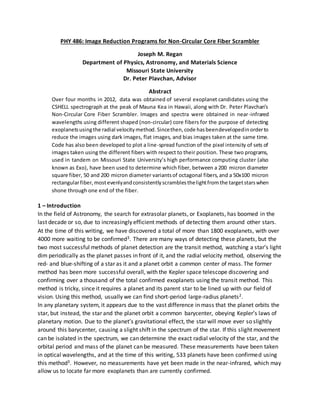
Figure 3: Image 5600 from May 10, 2012, showing the raw and reduced image ofthe 200 micron octagonal fiber, respectively.

7. Fig. 4: Line Spread Functions oftheeight main fibers,full plotand zoomedin. From top to bottom: 200 micron Octagonal 10m fiber, images
5540-5859;200MicronOctagonal1mfiber, images 4410-4729; 50 micron Octagonal10m fiber,images 4127-4316; 50 micron octagonal 1m
fiber, images 3884-3923; Rectangular 10m fiber,images 2496-2575; Rectangular1m fiber, images 3080-3239; Square 10mfiber, images 5184-
5402; Square 1m fiber, images 4823-4881
4.1 – Fiber Agitator
In all of the images used, while science data was being obtained, the fiber agitator was
turned on or off at some point. This was accounted for in the plotting of the data, but in nearly
all cases, the status of the agitator did not seemto have an effect on the shape of the line
spread function. In the case of images 4410-4569 and 4570-4729, the shape was affected
slightly and the standard deviation rose from 1.6% to 2.1%. This was the most significant
change brought on by the fiber agitator.

8. Fig. 5: On the top, Images 4410-4569 of the200 micron Octagonal1mfiber, withagitator on.On the bottom, Images 4570-4729 ofthe same
set, with agitator off. There is a slight change in the shape ofthe LSF, but nearly no change in the standard deviation oft he plots. Upon
inspecting the data, this is the set that was changed the most from the changing status ofthe fiber agitator. Below the images are their
respective zoomed-in plots.
4.2 – Standard Deviation
Also recorded were tables showing the implot commands for each data set in relation to
their fiber shape along with the standard deviation of each set. Data sets that included a change
in agitator status were split into three sets: one set with the agitator off, one with the agitator
on, and both combined, in order to compare standard deviations and shapes of each set when
plotted.
December’s data was split up into many individual ten-image data sets excluding a few,
notably images 1585-1695 on December 10th, the only images taken with the 50 micron
octagonal fiber, having a standard deviation of 16.89%. Upon inspection, none of the remaining
data taken on December 10th, all taken using the 200 micron octagonal 1m fiber, had standard
deviations of less than 14% ranging up to 26%.

9. Fig. 6: Typicalplot ofdata using the200micron Octagonal1m fiberon thenight ofDecember 10th. This particular data set: images 2344-2353.
On the night of December 11th, the data for the 200 micron octagonal 1m fiber was
taken in sets of twenty images rather than ten. The data was much more consistent towards
the end of the fiber’s run, eventually narrowing down to 1.8% standard deviation after starting
the run at about 14%. The rectangular 1m fiber, back to sets of ten images, showed some
consistency over the night, reading in standard deviations of about 2.2% at its best, but despite
being relatively consistent with the line spread function, the light was shown to be brighter
through the edge of the fiber than the core in most cases.
Fig 7: More stableplot ofdata using theRectangular 1m fiber on the night ofDecember 11th. This particular data set: Images 3507-3516.
The Square 1m fiber, also using ten-image sets, had by far the most consistency of the
three fibers used on December 11th, with the standard deviation ranging between 2.4% and 4%
and rarely stepping outside of that range. Over the course of the run, however, while the light
on the right side of the fiber stayed consistently bright, the light on the left side of the fiber
started out dim, but was even with the right side in brightness by the end of the run.

10. Fig. 8: Data using the Square1m fiberon thenight ofDecember11th. On theleft: Images 4227-4236. On the right, images 4337-4346.
8-May
Fiber Command Standard Deviation
200µm Oct 1m
implot,6418,6573 0.0364
implot,6681,6693 0.0267
implot,6694,6753 0.0888
implot,6754,6807 0.0437
implot,6845,6878 0.0084
implot,6845,6963 0.0446
implot,6879,6963 0.0521
implot,6979,6988 0.0185
implot,7013,7051 0.0446
200µm Oct
10m
implot,7227,7324 0.0875
implot,7449,7486 0.0138
9-May
Fiber Command Standard Deviation
200µm Oct 10m
implot,8735,8754 0.007
implot,8815,8894 0.319
200µm Oct 1m
implot,8352,8529 0.078
implot,8570,8589 0.021
implot,8655,8694 0.008
Rect 10m implot,258,265 0.011
Square 10m
implot,9495,9594 0.004
implot,9759,9838 0.011
Square 1m
implot,9035,9114 0.129
implot,9195,9394 0.041
10-May
Fiber Command Standard Deviation
200µm Oct 10m implot,5540,5699 0.0099

11. implot,5540,5859 0.0104
implot,5700,5859 0.0106
200µm Oct 1m
implot,4410,4569 0.016
implot,4410,4729 0.0234
implot,4570,4729 0.021
50µm Oct 10m
implot,4127,4206 0.0209
implot,4127,4316 0.0202
implot,4207,4316 0.0198
50µm Oct 1m
implot,3620,3699 0.032
implot,3620,3779 0.021
implot,3700,3779 0.0253
implot,3884,3923 0.0262
implot,3884,4003 0.119
implot,3924,4003 0.144
Rect 10m
implot,2068,2171 0.348
implot,2181,2233 0.0793
implot,2496,2575 0.01
implot,2767,2785 0.028
Rect 1m
implot,3080,3159 0.021
implot,3080,3239 0.022
implot,3160,3239 0.023
implot,3428,3507 0.132
implot,3428,3587 0.137
implot,3508,3587 0.144
Square 10m
implot,5184,5402 0.0112
implot,5404,5503 0.0118
Square 1m
implot,4823,4881 0.018
implot,4883,5142 0.023
As shown by the chart, the lowest standard deviation in any of the given data sets is the
Square 10m fiber, at 0.4% on May 9th, 2012. However, the only other data set with a standard
deviation less than 1% seems to be both of the 200 micron Octagonal fibers, with at least one
set showing sub-1% standard deviation each night in May between the two of them.
5 – Errors and Odd Data
There were a few notable errors in the plots due to the state of the raw images
themselves that caused inconsistency when reduced. It is uncertain what caused the errors, but
they were present during the gathering of the data.

12. Fig. 7: Data takenusing the Square1m fiberon May10th. The top plot,images 4823-5142, showoneplot outofplace. The bottom plots, from
left to right, show images 4823-4881 and images 4883-5142. Image 4882 was determined to be the error image.
Fig. 8: On the left,image4881from May 10th. In the middle, the imagein question, image 4882.Betweenthetwo images thereis a noticeable
odd area at boththetop andbottom ofthe second image. On the right, the averaged result ofthe two images, which would normally be
uniform in the case oftwo consistent images. It is uncertain what may have caused this error.

13. 6 – Code
Fig. 9: Image reductioncode,named impro2.pro. Process explained insection4, syntax detailed incommentsection atstart ofprogram.

17. Fig. 10: Program toplotthelinespreadfunction ofthereducedimages. Process includes summing inboth directions, normalization,and
calculation of standarddeviation.
7 – Conclusion
Code has been written for Missouri State University’s high-performance computing
cluster, Exo, to reduce images taken during several months’ time using Dr. Peter Plavchan’s
Non-Circular Core Fiber Scrambler at the CSHELL spectrograph on the top of Mauna Kea in

18. Hawaii. Code has also been written to plot the line spread function of pixel intensity with
respect to pixel position, with the purpose of determining the most reliable fiber core shape for
detecting exoplanets around M-Dwarf stars in the near-infrared using the radial velocity
method. After analyzing the data and determining the standard deviations of different sets of
data using different fiber shapes, it seems that all the fiber shapes have varying degrees of
reliability. However, by a small margin, it seems that the 200 micron Octagonal fibers, both the
1 and 10 meter variants, may be the most reliable fibers used in this analysis.
These plots and reduced images come from the two finished programs, unedited
throughout the process of reducing and plotting, and will require little to no upkeep as long as
the image sizes remain consistent using CSHELL. In the future the programs should be able to
quickly and efficiently reduce and analyze data taken using the CSHELL spectrograph or other
similar instruments that may replace it.
7 – References
1. Plavchan, P., et al., “Precision Near-Infrared Radial Velocity Instrumentation II: Non-Circular
Core Fiber Scrambler”, 2013, SPIE, in Optical Engineering + Applications, 8864 1J
2. Plavchan, P., et al., “Radial Velociy Prospects Current and Future,” 2015, ExoPAG Study
Analysis Group white paper
3. NASA Exoplanet Archive. 2015. Web.
<http://exoplanetarchive.ipac.caltech.edu/docs/counts_detail.html>