SlideShare a Scribd company logo
1 of 94
Download to read offline
Online Detection of Water Vapor in an
Industrial Gasifier Using Terahertz
Spectroscopy
Master’s Thesis in Physics and Astronomy
JENS NORDMARK
Department of Microtechnology and Nanoscience
Terahertz and Millimeter-wave Laboratory
Chalmers University of Technology
Gothenburg, Sweden 2013
Online Detection of Water Vapor in an Industrial Gasifier Using Terahertz Spectroscopy
Jens Nordmark
c Jens Nordmark, 2013
Terahertz and millimeter wave laboratory
Department of Microtechnology and Nanoscience
Chalmers University of Technology
SE-412 96 Gothenburg
Sweden
Abstract
A terahertz spectrometer was set up for the monitoring of product gas in a thermal gasi-
fier. The goal was to measure temperature and H2O concentration, and preferably also
CO concentration. This environment presents several difficulties such as high tempera-
ture, toxic gases, high H2O content and a high concentration of particulate pollutants.
Spectroscopy using IR Lasers tend to be obstructed by the high absorption of H2O as
well as the scattering by the particulates, and so does not produce satisfactory results.
It was hoped that these problems could be avoided by using terahertz radiation, with
a lower absorption by water and a longer wavelength possibly avoiding scattering by
particulates. A system operating in the range 300-500 GHz was built and tested in lab-
oratory as well as in an industrial gasifier at Chalmers Power center, yielding promising
results.
Our results indicate that monitoring of H2O, and probably other gases, in the rugged
environment of gasifier rawgas can be done with response times on the order of a few
minutes. This has applications in biomass gasification, where variable quality of the fuel
results in a need for continous monitoring and tuning of the gasification process.
Keywords: Terahertz, Gas spectroscopy, Gasification
Acknowledgements
I wish to thank my supervisor Sergey Cherednichenko for his help. I also wish to thank
Hosein Bidgoli and Martin Seeman at the department for energy and the environment
with whom the project was carried out. Also thanks to Johannes ¨Ohlin for assistance
during experiments at the Chalmers power center.
Jens Nordmark, Gothenburg July 1, 2013
Contents
Contents i
List of Tables iv
List of Figures vi
Nomenclature x
1 Introduction
1
1.1 Data . . . . . . . . . . . . . . . . . . . . . . . . . . . . . . . . . . . . . . . 4
2 Theory
5
2.1 Gasification of biomass . . . . . . . . . . . . . . . . . . . . . . . . . . . . . 5
2.2 Terahertz technology . . . . . . . . . . . . . . . . . . . . . . . . . . . . . . 9
2.2.1 H2O and CO absorption at Terahertz frequencies . . . . . . . . . . 9
2.2.2 Detectors and sources . . . . . . . . . . . . . . . . . . . . . . . . . 11
2.2.3 Waveguides . . . . . . . . . . . . . . . . . . . . . . . . . . . . . . . 13
2.3 Molecular spectroscopy . . . . . . . . . . . . . . . . . . . . . . . . . . . . . 14
2.3.1 Energy levels . . . . . . . . . . . . . . . . . . . . . . . . . . . . . . 14
The vibration-rotation spectrum of CO . . . . . . . . . . . . . . . 15
2.3.2 Line shape . . . . . . . . . . . . . . . . . . . . . . . . . . . . . . . 16
Natural broadening . . . . . . . . . . . . . . . . . . . . . . . . . . . 17
Doppler broadening . . . . . . . . . . . . . . . . . . . . . . . . . . 17
Collisional broadening . . . . . . . . . . . . . . . . . . . . . . . . . 17
Combined broadening . . . . . . . . . . . . . . . . . . . . . . . . . 17
Temperature dependence of line strength . . . . . . . . . . . . . . 18
Line-by-line models . . . . . . . . . . . . . . . . . . . . . . . . . . . 18
2.3.3 Collisional line mixing . . . . . . . . . . . . . . . . . . . . . . . . . 18
2.3.4 The HITRAN database . . . . . . . . . . . . . . . . . . . . . . . . 19
i
CONTENTS
2.3.5 LINEPAK vs custom algorithm . . . . . . . . . . . . . . . . . . . . 19
3 The setup
20
3.1 Gas cell design . . . . . . . . . . . . . . . . . . . . . . . . . . . . . . . . . 20
3.1.1 Window properties . . . . . . . . . . . . . . . . . . . . . . . . . . . 24
3.2 Spectrometer . . . . . . . . . . . . . . . . . . . . . . . . . . . . . . . . . . 26
3.2.1 Source . . . . . . . . . . . . . . . . . . . . . . . . . . . . . . . . . . 26
3.2.2 Detector: Golay cell . . . . . . . . . . . . . . . . . . . . . . . . . . 29
3.3 Humidity meter . . . . . . . . . . . . . . . . . . . . . . . . . . . . . . . . . 31
3.4 Spectrum analysis . . . . . . . . . . . . . . . . . . . . . . . . . . . . . . . 32
3.4.1 THz absorption by H2O vapors . . . . . . . . . . . . . . . . . . . . 32
3.4.2 THz absorption by Carbon Monoxide . . . . . . . . . . . . . . . . 32
4 Experimental methodology
35
4.1 Calibration . . . . . . . . . . . . . . . . . . . . . . . . . . . . . . . . . . . 35
4.2 Laboratory H2O measurements . . . . . . . . . . . . . . . . . . . . . . . . 37
4.3 Monitoring of H2O and CO at the gasifier . . . . . . . . . . . . . . . . . . 40
4.4 Noise and drifts . . . . . . . . . . . . . . . . . . . . . . . . . . . . . . . . . 44
5 Discussion
48
5.1 Detection of H2O . . . . . . . . . . . . . . . . . . . . . . . . . . . . . . . . 48
5.2 Detection of CO . . . . . . . . . . . . . . . . . . . . . . . . . . . . . . . . 51
5.3 Noise and drifts . . . . . . . . . . . . . . . . . . . . . . . . . . . . . . . . . 51
5.4 Other issues . . . . . . . . . . . . . . . . . . . . . . . . . . . . . . . . . . . 54
5.4.1 Temperature gradient and thermocouples . . . . . . . . . . . . . . 54
5.4.2 Line-by-line model vs LINEPAK . . . . . . . . . . . . . . . . . . . 54
5.5 Usability of the system . . . . . . . . . . . . . . . . . . . . . . . . . . . . . 54
Bibliography 57
A Line-by-line algortihm
60
B Line data from HITRAN2008
62
C SpectralCalc simulations
64
D Calculations of T and V MR from S380 and S448
70
D.1 Determination of T from measured V MR and S . . . . . . . . . . . . . . 70
ii
CONTENTS
D.2 Determination of V MR from calculated T and measured S . . . . . . . . 72
D.3 Simultaneous determination of T and V MR from S . . . . . . . . . . . . 73
E Humidity control
75
F Alternative waveguides
76
Index 77
iii
List of Tables
2.1 The expected contents of gasifier rawgas at Chalmers power center, based
on gas chromatography and H2O separation by condensation. All V MR
entries except H2O refer to dry gas composition. (Hosein Bidgoli, private
communication) . . . . . . . . . . . . . . . . . . . . . . . . . . . . . . . . . 6
2.2 The expected contents of gasifier fluegas at Chalmers power center, based
on gas chromatography and H2O separation by condensation. All V MR
entries except H2O refer to dry gas composition. (Hosein Bidgoli, private
communication) . . . . . . . . . . . . . . . . . . . . . . . . . . . . . . . . . 6
2.3 Detector types for far IR and THz. A summary of Rogalski and Sizov [2011] 12
2.4 Sensitivity for some detector types for far IR and THz. A summary of
Rogalski and Sizov [2011], last entry is a bolometer made at TML, MC2,
Chalmers. Described in Cherednichenko et al. [2011]. . . . . . . . . . . . . 12
3.1 Amplitudes of frequency swings due to modulation with various ampli-
tudes. ∆fin is the maximum deviation from the mean frequency at any
particular value of the control voltage Uctrl, and is due to the value of
the FM voltage UFM. ∆fout is the output frequency of the AMC after
multiplication. The relation between FM modulation voltage and output
frequency swing varies slightly across the operating range of our source,
as can be seen in the difference in output from these two control voltages
when all other parameters are kept constant. . . . . . . . . . . . . . . . . 27
3.2 Coefficients for the Antoine equation for H2O, from DDBST [2013]. . . . 31
4.1 Transmissions obtained at different humidity levels in two separate mea-
surements of the type shown in figure 4.2. Errors are shown as one stan-
dard deviation. Measurement number indicates which of the two separate
dataseries the entry comes from. . . . . . . . . . . . . . . . . . . . . . . . 37
iv
LIST OF TABLES
5.1 Temperature estimations using least-squares from the data in table 4.1.
The calculation is shown in appendix D. Errors are given as one standard
deviation. The last column shows how V MR is calculated assuming the
calculated temperature and measured transmissions. . . . . . . . . . . . . 50
5.2 The result when fitting both T and V MR using the program in appendix
D.3, and the same data as in the table above. . . . . . . . . . . . . . . . . 50
B.1 Spectral lines of CO . . . . . . . . . . . . . . . . . . . . . . . . . . . . . . 62
B.2 Spectral lines of water . . . . . . . . . . . . . . . . . . . . . . . . . . . . . 63
F.1 Transmission at three distances with and without waveguide, normalized
to the 10 cm air transmission. . . . . . . . . . . . . . . . . . . . . . . . . . 76
v
List of Figures
1.1 Scattering cross-section as function of frel = R/λ for a spherical particle.
Calculated with MiePlot 4.3 by Laven [2013], implementing the BHMIE
algorithm by Bohren and Huffman [2007]. [data/mie] . . . . . . . . . . . . 2
1.2 The spectra of two gas mixtures at room temperature (296 K). 10% H2O
(blue) and 10% H2O+10% CO (red). [data/introspectrum] . . . . . . . . 2
1.3 The simulated spectra of H2O at V MR = 20% and varying temperatures.
[data/AppendixC] . . . . . . . . . . . . . . . . . . . . . . . . . . . . . . . 3
1.4 The simulated spectra of H2O at T = 573K and varying humidity. [data/AppendixC] 3
2.1 The device measuring H2O content by condensation. H2O and tar con-
dense while bubbling up from the bottom of the isopropanol pool, and
mix with the liquid. The mass increase of the isopropanol container gives
the amount of H2O and tar in a volume of gas, ∆m = mH2O + mtar. To
give a good accuracy, the mass increase must be measured over periods
of several hours. . . . . . . . . . . . . . . . . . . . . . . . . . . . . . . . . 6
2.2 The operating principle of the Chalmers gasifier . . . . . . . . . . . . . . . 8
2.3 Top: Spectra of 10% H2O and 10% CO + 10% H2O in the range 100GHz
to 1 THz at 296 K. Bottom: The same restricted to 300-500 GHz. [data/simulation
full] . . . . . . . . . . . . . . . . . . . . . . . . . . . . . . . . . . . . . . . 10
2.4 vibrational modes and rotational axes of CO and H2O . . . . . . . . . . . 15
2.5 Sketch of typical rovibrational spectrum for a diatomic molecule with a
vibrational transition at 1000, and rotational constant of 1/2, in arbitrary
units. . . . . . . . . . . . . . . . . . . . . . . . . . . . . . . . . . . . . . . 16
2.6 The type of transitions giving rise to line mixing. . . . . . . . . . . . . . . 19
3.1 A sketch of the gas cell . . . . . . . . . . . . . . . . . . . . . . . . . . . . . 21
3.2 The gas cell and its connections to the rest of the system. . . . . . . . . . 21
3.3 The gas cell set up at the gasifier . . . . . . . . . . . . . . . . . . . . . . . 22
3.4 The gas cell in the lab within the closed oven, tubing and electronics. . . 22
3.5 The gas cell inside the open oven . . . . . . . . . . . . . . . . . . . . . . . 23
vi
LIST OF FIGURES
3.6 Transmission through teflon(top) and quartz(bottom) windows at normal
incidence relative to air. [data/windowproperties/] . . . . . . . . . . . . . 25
3.7 The setup of the instruments around the gas cell . . . . . . . . . . . . . . 26
3.8 A nitrogen spectrum in terms of control voltage vs output voltage from
the Golay cell. The voltage span corresponds to a full frequency sweep
over 300-500 GHz. Note the very high sensitivity to small variations
in the contol voltage. This sensitivity motivated the use of frequency
modulation. [data/ctrl-to-signal] . . . . . . . . . . . . . . . . . . . . . . . 27
3.9 Sketch of the setup of the source, from VDI manual. . . . . . . . . . . . . 28
3.10 Source power output, from VDI manual. . . . . . . . . . . . . . . . . . . . 28
3.11 Sketch of the Golay cell . . . . . . . . . . . . . . . . . . . . . . . . . . . . 29
3.12 Left: Golay cell. Right: The microwave source . . . . . . . . . . . . . . . 30
3.13 The Amplifier multiplier chain, concealed within a black box. . . . . . . . 30
3.14 Line positions and intensities for H2O. Upper left: 0-40 cm−1 with cutoff
at intensity < e−23. Upper right: 0-40 cm−1 with no cutoff. Lower left:
10-16.7 cm−1 with cutoff at intensity < e−23 Lower right: 10-16.7 cm−1
with no cutoff. Compare figure 2.3. . . . . . . . . . . . . . . . . . . . . . . 33
3.15 Line positions and intensities for CO. Upper left: 0-40 cm−1 with cutoff
at intensity < e−23. Upper right: 0-40 cm−1 with no cutoff. Lower left:
10-16.7 cm−1 with cutoff at intensity < e−23 Lower right: 10-16.7 cm−1
with no cutoff. Compare figure 2.3. . . . . . . . . . . . . . . . . . . . . . . 34
4.1 Top: Two raw measurements, one of N2 which lacks spectral lines in this
frequency range to be used for calibration, and one of gasifier rawgas. Bot-
tom: The transmission spectrum formed by dividing the rawgasspectra
by the calibration spectra. V MR ≈ 65% and T ≈ 430oC. [data/rawspectra] 36
4.2 Top: the two water lines are plotted as functions of time, where the
H2O content is changed in steps. Bottom: the humidity meter gives the
corresponding V MR. [data/twolines] . . . . . . . . . . . . . . . . . . . . . 38
4.3 Laboratory measurement of transmission at 449 GHz over time for five
humidity levels. The impulse-like objects are products of the humidifier,
it seems to release steam in short pulses. Note that measurements with
a difference in V MR as small as 0.4% can be clearly distinguished from
each other. [/data/20130204] . . . . . . . . . . . . . . . . . . . . . . . . . 39
4.4 The spectrum of the rawgas, 300-500 GHz. Note the CO line at 460 GHz.
Also included is a fluegas measurement at 410-470 GHz. Spectralcalc
simulations for the rawgas are also included, compare table 2.1 of rawgas
contents. [data/rawgasplot] . . . . . . . . . . . . . . . . . . . . . . . . . . 41
4.5 Raw and fluegas from the same measurement as above, zoomed in on the
H2O-line at 448 GHz.[data/rawgasplot] . . . . . . . . . . . . . . . . . . . 41
4.6 H2O (41%) compared to H2O (41%) and CO (20%). [/data/coandh2o] . 42
vii
LIST OF FIGURES
4.7 Measurement over time of the 448 GHz transmission at the gasifier. Vary-
ing the steam input of the process: 160, 200, 240, 160, 120 kg/h. [data/gasifier-
humiditylevels] . . . . . . . . . . . . . . . . . . . . . . . . . . . . . . . . . 43
4.8 N2 spectra taken over a period of four hours for the gas cell at room
temperature and normalized to the first one of them. Moving average
over 15 GHz.[data/drifts/book3-20130311] . . . . . . . . . . . . . . . . . . 45
4.9 N2 spectra taken over a period of eight hours at high temperature (oven
at 600 C) and normalized to the first one of them. The legend shows
the time that the corresponding measurement was taken. Moving average
over 15 GHz.[data/drifts/book1-20130312] . . . . . . . . . . . . . . . . . . 46
4.10 N2 spectra taken over a period of five hours at high temperature (oven
at 600 C) and normalized to the first one of them, with better thermal
isolation (10 cm more air between source and gas cell) than in figure 4.9.
Moving average over 15 GHz.[data/drifts/book2-20130327] . . . . . . . . . 46
4.11 Noise plot in the lab obtained by division of two subsequent N2-spectra.
Integration time 100 ms. Note that signal strength approaches zero at
the ends of the spectrum, causing signal-to-noise ratio to decrease. In
this plot no smoothing has been used. [data/noise] . . . . . . . . . . . . . 47
4.12 Noise plot at the gasifier obtained by division of two subsequent N2-
spectra. Integration time 100 ms. In this plot no smoothing has been
used. [data/noise] . . . . . . . . . . . . . . . . . . . . . . . . . . . . . . . . 47
5.1 Transmission as function of temperature calculated by the line-by-line-
model for the V MR of 73% detected in the measurements of figure . The
black lines show where the measured transmissions intersect the simula-
tion, giving the temperature. The values of T should coincide, but do not.
Precise estimates from a least-squares fit for several measurements of this
type are shown in table 5.1. [data/temp humidity] . . . . . . . . . . . . . 49
5.2 Transmission as function of temperature calculated by Spectralcalc for the
V MR of 73% detected in the measurements of figure . The black lines
show where the measured transmissions intersect the simulation, giving
the temperature. The values of T should coincide, but do not. The
temperatures differ much more than above. [data/temp humidity] . . . . 49
5.3 An N2 measurement at 383 GHz with 300 millisecond integration time
and one data point taken per second, in the lab.[data/rmsd] . . . . . . . . 52
5.4 Allan variance of the above signal.[data/rmsd] . . . . . . . . . . . . . . . . 52
5.5 The 449 GHz line from rawgas at the gasifier (200 kg/h of H2O), mon-
itored for 1200 seconds. 100 millisecond integration time and one data
point taken per 300 milliseconds.[data/rmsd] . . . . . . . . . . . . . . . . 53
5.6 Allan variance of the above signal. [data/rmsd] . . . . . . . . . . . . . . . 53
5.7 A comparison of rawgas measurment, spectralcalc and line-by-line simu-
lation. [data/comparison] . . . . . . . . . . . . . . . . . . . . . . . . . . . 55
viii
LIST OF FIGURES
C.1 The simulated spectra of H2O at V MR = 20% and varying temperatures.
[data/AppendixC] . . . . . . . . . . . . . . . . . . . . . . . . . . . . . . . 65
C.2 The simulated spectra of H2O at T = 573K and varying humidity. [data/AppendixC] 65
C.3 Ratio of H2O peak transmission at 448 and 383 as function of temperature
when V MR is kept constant at 20%. [data/AppendixC] . . . . . . . . . . 66
C.4 Ratio of H2O peak transmission at 448 and 383 as function of V MR when
T is kept constant at 573 K. [data/AppendixC] . . . . . . . . . . . . . . . 66
C.5 The simulated transmission of H2O at 380 GHz for various T and V MR.
[data/AppendixC] . . . . . . . . . . . . . . . . . . . . . . . . . . . . . . . 67
C.6 The simulated transmission of H2O at 448 GHz for various T and V MR.
[data/AppendixC] . . . . . . . . . . . . . . . . . . . . . . . . . . . . . . . 67
C.7 The simulated transmission at 380 GHz, dependence on T for 10 different
values of H2O V MR. [data/AppendixC] . . . . . . . . . . . . . . . . . . . 68
C.8 The simulated transmission at 448 GHz, dependence on T for 10 different
values of H2O V MR. [data/AppendixC] . . . . . . . . . . . . . . . . . . . 68
C.9 The simulated transmission at 380 GHz, dependence on H2O V MR for
12 different values of T. [data/AppendixC] . . . . . . . . . . . . . . . . . 69
C.10 The simulated transmission at 448 GHz, dependence on H2O V MR for
12 different values of T. [data/AppendixC] . . . . . . . . . . . . . . . . . 69
ix
Nomenclature
CH4 Methane
CO Carbon monoxide
CO2 Carbon dioxide
H2 Hydrogen
RH Relative Humidity, ratio of H2O partial pressure to saturated vapor
pressure.
V MR Volume Mixing Ratio
AMC Amplifier-/Multiplier Chain
EM Electromagnetism, Electromagnetic
GPIB General purpose interface bus, same as IEEE 488
HITRAN high-resolution transmission molecular absorption database
IEEE Institute of Electrical and Electronics Engineers
IEEE 488 General purpose interface bus, GPIB
IR Infrared
LINEPAK Software library for spectral simulation described in Gordley et al. [1994].
NEP Noise Equivalent Power
RMSD Root Mean Square Deviation
SNG Substitute Natural Gas, methane
tar A loosely defined viscous black substance consisting mainly of large
hydrocarbons, often aromatic, polycyclic and containing various sub-
stituents.
THz TeraHertz
TTL Transistor-Transistor Logic, a binary logic scheme using 0-0.8 V signals
for low and 2.2-5 V for high
x
1
Introduction
Gasification of biomass is a technology expected to become more important as fossil
fuels are to be replaced by carbon neutral bioenergy. The company WSP has made
projections based on three scenarios, showing a potential for up to 12 TWh in biogas
production by thermal gasification up to 2030 under favorable conditions. Distribution
of the combustible gas produced (typically SNG, i.e. methane) could take place using
the present natural gas infrastructure (Dahlgren et al. [2013]).
The properties of the fuels used are however such that the producer gas, also called
rawgas in the stage immediately after it is generated, is full of char particles at sizes up
to about one micron. At the same time its gas contents vary in time, and need to be
tracked to tune the process. The particulate contents as well as the high H2O content
disturb the IR-spectroscopy that would typically be used to monitor gas content. H2O
simply has to high absorption in the IR for such radiation to be used successfully. The
wavelength of IR is also at the order of the particulates diameter, giving rise to scatter-
ing that disrupts measurements. Gas chromatography is another technique traditionally
used, but it cannot handle gas mixtures containing H2O, which condenses in the chro-
matograph and destroys it. It is possible to measure the dry gas composition by first
drying and cleaning the gas. This also provides a way to determine the sum of H2O and
tar contents, but only the total content and not both independently. In addition, it only
works with a time delay of tens of minutes.
As an alternative solution, this project aimed to use terahertz spectroscopy in the
hope to escape the aforementioned problems. Our aim was to measure content of H2O
as well as CO, one of the dry gases present. Our results indicate that this approach does
work as desired.
There are several reasons why this approach succeeds. THz has a lower absorption
for H2O, avoiding saturation of the spectral lines. THz has longer wavelengths than
IR, which reduces the scattering by particulates. The scattering of radiation by ideal
spherical particles is described by Mie theory, where a threshold in the scattering cross
1
CHAPTER 1. INTRODUCTION
1.00EͲ11
1.00EͲ09
1.00EͲ07
1.00EͲ05
1.00EͲ03
1.00EͲ01
1.00E+01
1.00E+03
0 0.5 1 1.5 2 2.5 3
Cross section
Scatterer size (Radius/wavelength)
Figure 1.1: Scattering cross-section as function of frel = R/λ for a spherical particle.
Calculated with MiePlot 4.3 by Laven [2013], implementing the BHMIE algorithm by Bohren
and Huffman [2007]. [data/mie]
0.5
0.6
0.7
0.8
0.9
1
300 320 340 360 380 400 420 440 460 480 500
Transmission
Frequency [GHz]
H2O+CO
H2O
Figure 1.2: The spectra of two gas mixtures at room temperature (296 K). 10% H2O
(blue) and 10% H2O+10% CO (red). [data/introspectrum]
section appears when the wavelength is comparable to the size of the scatterers, which
can be formulated in terms of the relative frequency frel = R/λ ≈ 1/2 as shown in figure
1.1. In the low frequency limit, there is weak Rayleigh scattering that decreases quickly
with particle size, while in the optical limit of large frel the scattering cross section is
close to 1. By increasing λ we decrease relative frequency (frel) and thus move closer to
the Rayleigh limit. This was one of the motivations for using THz radiation.
Spectroscopy in field environments using terahertz has been demonstrated in several
applications, for instance the remote detection of chemicals in Gopalsami et al. [2008]
or the remote detection of nuclear radiation in Gopalsami et al. [2009]. Currently the
spectra of H2O as well as that of CO in the region 300-500 GHz are well known and
included in the HITRAN database. This spectral range contains a few strong H2O lines
and a few conveniently places CO lines, shown in figure 1.2.
The absorption at the line centers is dependent on both concentration and tem-
2
CHAPTER 1. INTRODUCTION
perature as shown in figures 1.3 and 1.4. Thus it is possible to determine these two
parameters from measured spectra.
Figure 1.3: The simulated spectra of H2O at V MR = 20% and varying temperatures.
[data/AppendixC]
Figure 1.4: The simulated spectra of H2O at T = 573K and varying humidity.
[data/AppendixC]
3
1.1. DATA
CHAPTER 1. INTRODUCTION
1.1 Data
Some of the data and code used for obtaining the figures in the text has been put in the
following Google Drive folder:
https://drive.google.com/folderview?id=0B25vmzARFvvOdnlYNDBocEFQNGM
4
2
Theory
2.1 Gasification of biomass
Production of combustible gas from biomass can be achieved using several processess,
including biological and thermal. In the present project, we are concerned with thermal
gasification of biomass, particularly from wood pellets. However, many types of high-
grade biomass are required in other industries and the energy sector will have to settle for
the leftovers. Thus it will be necessary to handle a highly variable input in a process. This
is why online detection of the product is required, since the process must be continuosly
tuned to the variable input.
In thermal gasification the solid biomass is broken down thermally in the presence of
an oxidising agent, in this case H2O. The main products are CO, CO2, H2, CH4, tars
and other hydrocarbons. The dry gases and the water contents expected in the rawgas
of the Chalmers gasifier are given in table 2.1, and for the fluegas data are given in table
2.2. Primary tars are of the form CxHyOz, but are themselves broken down into either
new tars, H2 or the product gases mentioned. The process requires a temperature above
600oC. (Gomez-Barea and Leckner [2010]).
The H2O content is of critical importance in regulating the rate of the process, since
it is involved in most reactions breaking down the large molecules of the fuel into product
gas. The contents of the gas must be very finely tuned for downstream processes to work,
which requires a low-delay monitoring of the most significant species. The intended
downstream process in this case is generation of substitute natural gas (SNG), by the
process of water gas shift:
3H2 + CO → CH4 + H2O (2.1)
This is highly sensitive to the ratio of CO to H2.
5
2.1. GASIFICATION OF BIOMASS
CHAPTER 2. THEORY
Table 2.1: The expected contents of gasifier rawgas at Chalmers power center, based on
gas chromatography and H2O separation by condensation. All V MR entries except H2O
refer to dry gas composition. (Hosein Bidgoli, private communication)
Gas H2 CO CO2 CH4 C2H2 C2H4
V MR [%] 4.64 23.40 35.50 16.35 13.78 0.33
Gas (cont.) C2H6 C3H6 C3H8 He N2 H2O
V MR [%] 0.70 0.47 0.02 1.11 3.42 ca 65
Table 2.2: The expected contents of gasifier fluegas at Chalmers power center, based on
gas chromatography and H2O separation by condensation. All V MR entries except H2O
refer to dry gas composition. (Hosein Bidgoli, private communication)
Gas N2 O2 CO2 H2O
V MR [%] 79.5 3.5 17 ca 20
Figure 2.1: The device measuring H2O content by condensation. H2O and tar condense
while bubbling up from the bottom of the isopropanol pool, and mix with the liquid. The
mass increase of the isopropanol container gives the amount of H2O and tar in a volume of
gas, ∆m = mH2O + mtar. To give a good accuracy, the mass increase must be measured
over periods of several hours.
6
2.1. GASIFICATION OF BIOMASS
CHAPTER 2. THEORY
Other methods than THz spectroscopy to monitor H2O are IR spectroscopy or con-
densation (explained in figure 2.1). IR spectroscopy has the problems of increased scat-
tering by the particulates, due to the shorter wavelength of IR compared to terahertz.
The absorption of water is also very high in the IR, creating a risk of saturation of such
spectrometers. Condensation is more robust: just let the H2O condense and compare its
mass to the volume of gas it came from. But this creates a long delay and also fails to
differentiate between H2O and tar, since tar also condenses. This motivates the attempt
to use THz instead.
A gasifier has a bed of material with high heat capacity to keep the fuel at an even
temperature. There are several designs of these beds, in the Chalmers case it is a fluidized
bed, made of sand that has properties resembling a fluid when under the conditions of
the gasifiers operation. The fuel is mixed with the bed material. Heat is provided
by a separate combustion chamber, this is called external heating to differentiate from
the case where the gasifier itself provides heat. Bed material is continously circulated
between combustion chamber and gasifier to provide heat. Bubbles of steam will move
upward through the bed material, accumulating gasifier products along the way. At this
stage the particulates in the gas are small, submicron size, so they will not affect the THz
radiation much. The temperature of flue- and rawgas leaving the gasifier is anticipated
to be around 850o C, which is the operating temperature of the process, but it cools
down to about 350o C before reaching the gas cell, since it is transported in heating
hoses with a capacity of maximum 350o C. It is then heated again inside the oven to
430o C to avoid condensation in the gas cell.
Figure 2.2 shows a flow diagram of the process at the Chalmers gasifier. Fuel is
fed from above into both chambers. In the combustion chamber, air is injected for
combustion while in the gasification chamber steam, the oxidizing agent, is inserted
instead. Heat is transported from the combustion chamber to the gasification chamber
by circulation of the hot sand of the fluidized bed. The output gas of the combustor is
referred to as fluegas, while the product gas of the gasifier is called rawgas when it is
leaving the gasifier, before being cleaned for downstream use.
7
2.1. GASIFICATION OF BIOMASS
CHAPTER 2. THEORY
Figure 2.2: The operating principle of the Chalmers gasifier
8
2.2. TERAHERTZ TECHNOLOGY
CHAPTER 2. THEORY
2.2 Terahertz technology
The terahertz region of the electromagnetic spectrum is defined as wavelengths from
3mm to 30 µm. It starts at the upper edge of millimeter waves and ends at the lower
edge of the infrared. Generation and detection of radiation in this range is more difficult
than in the microwave region of the EM spectrum, and THz equipment is currently an
area of intense research.
Several applications of THz radiation exploit its ability to penetrate tissue, fabric and
plastics to a significant depth, while being partially reflected depending on density and
contents of objects. This makes possible a variety of imaging applications. In addition,
it is non-ionizing1 and thus harmless to living organisms unless used with very high
power output, which tends to be neither needed nor available. In the present project,
we attempted to exploit THz radiation in the monitoring of water vapor content in dirty
gasifier rawgas, where IR laser spectroscopy fails due to the particulate matter in the
gas. THz was expected to pass through the particulates. We also face the issue of
high temperatures. Temperature affects spectral lines both by changing their relative
strengths and by broadening of lines. This is further described in section 2.3.2.
2.2.1 H2O and CO absorption at Terahertz frequencies
We need to detect H2O under various concentrations and temperatures. It is important
to avoid saturation of the spectrometer. In figure 2.3 we show the spectra of H2O as
well as CO. Three of the H2O lines are very strong and risk to saturate our system. We
want several weak lines in the frequency range used. The band 300-500 GHz suits this
purpose for both gases considered, and equipment for sweeping over these frequencies
exists. The danger of saturation is exacerbated by high temperatures, which increase
absorption significantly. See appendix C for plots of the temperature dependence of
absorption at various concentrations of H2O.
1
Photon energies vary from 0.413 meV at 3 mm to 41.3 meV av 30 µm
9
2.2. TERAHERTZ TECHNOLOGY
CHAPTER 2. THEORY
0
0.1
0.2
0.3
0.4
0.5
0.6
0.7
0.8
0.9
1
1002003004005006007008009001000
Transmission
Frequency [GHz]
H2O+CO
H2O
0.9
0.91
0.92
0.93
0.94
0.95
0.96
0.97
0.98
0.99
1
300320340360380400420440460480500
Transmission
Frequency [GHz]
H2O+CO
H2O
Figure2.3:Top:Spectraof10%H2Oand10%CO+10%H2Ointherange100GHzto1THzat296K.Bottom:Thesame
restrictedto300-500GHz.[data/simulationfull]
10
2.2. TERAHERTZ TECHNOLOGY
CHAPTER 2. THEORY
2.2.2 Detectors and sources
Detectors for THz can be broadly categorized into thermal or photon detectors, as Ro-
galski and Sizov [2011] describe. Thermal detectors absorb the radiation and gain heat,
which induces change in some physical property of the material that can be easily mea-
sured. For instance, metals or semiconductors can be used that change their electrical
conductivity in response to temperature differences. This is a common category of de-
tectors called Bolometers. Another example would be to measure the thermal expansion
of a gas, which is the method we use. That type of detector is called a Golay cell and
is described in detail in section 3.2.2. Thermocouples are devices that generate voltage
over a junction of two different materials in response to temperature changes. They are
used in many applications and can be used as IR detectors as well as for temperature
measurements in general.
Photon detectors rely on excitations in semiconductors. When a photon is absorbed
its energy gives rise to an electron-hole pair. These gives rise to electrical conduction, in
a variety of ways for different detector types. They have a frequency-dependent response,
unlike thermal detectors. Their advantage is that they tend to have very fast response
times and good signal-to-noise ratio. A major inconvenience is that they require cooling
to very low temperatures to avoid thermally generated noise. A thermal detector is for
this reason the favoured option provided that its precision is acceptable. The Golay cell
was used because it was available. We list some detector types in table 2.3. A measure
of detector sensitivity in common use is Noise Equivalent Power, NEP. It is defined as
the power required of an input signal to generate a signal-to-noise ratio of 1 in an output
signal with 1 Hz bandwidth. The unit is W /
√
Hz. This should of course be as low as
possible for good detectors. A few examples from Rogalski and Sizov [2011] are collected
in table 2.4. A higher sensitivty of a detector lessens the noise and shortens the required
integration time at a particular noise level.
11
2.2. TERAHERTZ TECHNOLOGY
CHAPTER 2. THEORY
Table 2.3: Detector types for far IR and THz. A summary of Rogalski and Sizov [2011]
Category Detector type Mechanism
Thermal Bolometers Temperature dependence of conductivity
Thermocouple Voltage generated by temperature change
Pyroelectric Charged plane conductors changing polarity
Golay cell Thermal expansion of gas
Photon Photoconductors Photon absorption in energies above the band gap cre-
ates carrier/hole pair in a uniform piece of some semi-
conductor, raising conductivity.
p-n junction diodes Photon-induced pair production creates a photocur-
rent across a junction between p- and n-doped semi-
conductors
Schottky barrier diodes Photocurrent across Schottky barrier
Table 2.4: Sensitivity for some detector types for far IR and THz. A summary of Rogalski
and Sizov [2011], last entry is a bolometer made at TML, MC2, Chalmers. Described in
Cherednichenko et al. [2011].
Detector type NEP [W /
√
Hz]
Golay cell 10−9 − 10−10
Schottky diode 10−10, increasing with ν
Bi bolometer 1.6 × 10⁻¹⁰, increasing with ν
Nb microbolometer 5 × 10⁻¹¹
Ti microbolometer 4 × 10⁻¹¹
Ni microbolometer 1.9 × 10⁻¹¹
YBCO bolometer 3.7 × 10⁻¹⁰
12
2.2. TERAHERTZ TECHNOLOGY
CHAPTER 2. THEORY
2.2.3 Waveguides
Waveguides are conducting tubes used to transfer radiation with as little attenuation as
possible. Their dimensions are chosen with respect to the wavelength of the radiation
considered, and longer wavelengths require broader waveguides. Each waveguide geom-
etry has a cutoff frequency below which decay of the transmitted wave will occur. All
waveguides that are not perfect conductors will experience attenuation, which is lower
for higher frequencies. The minimum attenuation naturally occurs for an infinitely large
waveguide, but detector apertures tend to be quite small and one needs to balance these
two requirements. Conical horns at the end of the waveguide is one way of balancing
these needs. Waveguides at which the intended wavelength is small enough to allow
”overmoding”, where many additional modes of propagation can occur, are called over-
sized waveguides. These give a low attenuation, but less mode purity. Such a waveguide
was used in this project. It is oversized since it has an internal diameter of 26 mm while
the longest wavelength used is 1 mm. In our case only the total transmitted energy is
measured, the Golay cell treats all modes of propagation equally, so overmoding is not
a big problem.
13
2.3. MOLECULAR SPECTROSCOPY
CHAPTER 2. THEORY
2.3 Molecular spectroscopy
When EM radiation passes through a sample, its rate of transmission will depend on
various properties of the sample. The Beer-Lambert law formulates this as:
T = T0e−Al
(2.2)
where l is the length of the sample along the beam and A is an absorption coefficient, de-
pending of a number of parameters. Since these parameters are specific to the substances
in a sample, as well as to some other conditions such as pressure and temperature, one
can infer facts about the sample by studying its absorption spectrum. Calculating the
absorption in relation to the pressure, temperature and composition is the subject of the
following sections.
2.3.1 Energy levels
In an atom there are only electronic energy levels, which usually have optical transitions.
Some fine structure transitions are in the terahertz, though. When forming a molecule,
valence electrons of the constituent atoms will inhabit molecular orbitals instead of
the atomic orbitals, with somewhat different energies. But there are also new degrees
of freedom present. Molecules do not have rotational symmetry and will thus have
rotational energy. The rotation must be treated quantum mechanically by rewriting the
expression for rotational energy with quantum mechanical operators, and this gives rise
to quantized rotational states. This will be demonstrated for CO below. Each molecular
bond will in addition introduce vibrational modes, giving a spectrum of vibrational
states. The number of vibrational modes depends on the molecule. A diatomic molecule
such as CO has only one vibrational mode, while water is more complicated and has
three vibrational modes. A sketch of the various modes of the two molecules is given in
figure 2.4.
To calculate electronic energy levels in molecules one uses the Born-Oppenheimer
approximation: nuclear and electronic motion are assumed to be completely separate.
This is justified since electron mass is about two thousandths of the mass of a nucleon,
thus moving much quicker. In effect, electron wavefunctions depend only on the position
of the nuclei and the motion of the nuclei depends only on the time-averaged distribution
of electrons. Another approximation that might be used is to consider the molecule a
rigid rotor when calculating rotational energy levels. Without this assumption there is
some vibration-rotation coupling. This is however true to a significant degree at higher
energy levels and then the rigid rotor approximation has to be abandoned. Vibration
can be modeled as a harmonic oscillator for low energy levels, but at high energy levels
it must be replaced by an anharmonic oscillator that couples to the rotation.
While rotation-vibration in diatomic molecules can be handled analytically with ease
the difficulty increases enormously for even triatomic molecules such as water. Theses
are written on this subject, for instance Lori [2008]. A basic description of the vibrational
levels would be a linear superposition of single-mode vibrations, but calculating exact
levels requires handling nonlinear effects. We instead describe the diatomic molecule.
14
2.3. MOLECULAR SPECTROSCOPY
CHAPTER 2. THEORY
Figure 2.4: vibrational modes and rotational axes of CO and H2O
The vibration-rotation spectrum of CO
Vibration of CO is modeled as a harmonic oscillator for low energy levels (McQuarrie
[2008], chapter 5), so the energy levels are of the form Evib = (ν + 1
2)¯hω where ω = k
µ
is determined empirically. µ is the reduced mass and k is the bond force constant. These
lines generally are in the infrared. For CO, ν = 1 → 2 is at 269 meV or 65 THz.
Rotation of CO is modeled as a rigid rotor with length re, the interatomic distance
at equilibrium. Its moment of inertia, with respect to a line normal to the bond and
intersecting it at the center of mass, is then given by I = µr2
e where µ is the reduced
mass of the two-body system. We can insert this in the Schr¨odinger equation expressed
in terms of the angular momentum operator J:
J2
2I
ψ = Erotψ (2.3)
with eigenvalues Erot = ¯h2
2I j(j +1). In the case of CO we do not have to worry about the
other rotational axes, one is identical and the other is a symmetry axis. Inserting the
parameters for CO (from Hush and Williams [1974]) gives Erot = 0.24j(j +1)meV . This
15
2.3. MOLECULAR SPECTROSCOPY
CHAPTER 2. THEORY
Figure 2.5: Sketch of typical rovibrational spectrum for a diatomic molecule with a vibra-
tional transition at 1000, and rotational constant of 1/2, in arbitrary units.
is a multiple of about 58 GHz, starting in the microwave region. It is not surprising that
rotational lines are also present in the neighboring THz region. The energy of the tran-
sitions has a clear hierarchy, electronic>vibrational>rotational. Rotiational transitions
are on the order of 1-10 cm−1 compared to about 1000 cm−1 for vibrational transitions.
For each vibrational level one can thus superimpose rotational transitions and get a
spectrum such as that sketched in figure 2.5. Selection rule ∆J = 0 suppresses the pure
vibrational transition, which is surrounded by two branches of rotational transitions,
the lower energy P-branch for ∆J = −1 transitions and the higher energy R-branch of
∆J = 1.
Similar principles apply for the water molecule, but the calculations are very involved.
Both CO and H2O have rotational lines in the region 300-500 GHz, where we have
measured. See figure 3.15 for the rotational lines of CO. They can be easily understood,
while the H2O lines in figure 3.14 are more complex. In practical applications one uses
semiempirical rather than calculated spectra.
2.3.2 Line shape
The line shape is affected by pressure- and temperature induced broadening, tempera-
ture dependences in line strength, and line mixing. There are three main types of line
broadening (Liou [2002], chapter 1):
• Natural broadening: due to the time-energy uncertainty principle.
• Doppler broadening: due to doppler shifts of the radiation from sources moving in
all directions.
• Pressure broadening: due to several pressure-dependent effects including collisions
(shortening excited state lifetimes) and perturbations of the energy levels of atoms
by the electric fields of nearby atoms.
We briefly describe these types to show which are important in our case.
16
2.3. MOLECULAR SPECTROSCOPY
CHAPTER 2. THEORY
Natural broadening
This type of broadening is the most fundamental, existing due to the Heisenberg uncer-
tainty principle:
∆E∆t ≥ h/2π (2.4)
The lifetime of a state is thus inversely proportional to its uncertainty in energy. Unless
states in the gas are extremely short-lived, this is completely negligible.
Doppler broadening
The velocity of molecules in a gas follow a Maxwell distribution:
p(v) =
1
√
πv0
ev2/v0
(2.5)
where v0 is the mean speed given by v0 = 2kBT/m. This gives rise to a Gaussian
lineshape:
fD(ν − ν0) =
1
αD
√
π
exp −
(ν − ν0)2
α2
D
(2.6)
where αD = ν0
2kBT
mc2 . This type of broadening is significant at very high temperatures
or at low pressures, and the temperatures in our case might be high enough.
Collisional broadening
Collisional broadening follows a Lorentz line shape:
f(ν − ν0) =
α/π
(ν − ν0)2 + α2
(2.7)
where
α = α0
p
p0
T0
T
n
(2.8)
Where α0 is the halfwidth at reference temperature T0. The half-width is composed of
the self- and foreign-broadened halfwidths, that are added with weighting in accordance
with the volume mixing ratio (V MR) of the gases present. This type of broadening
is very significant in atmospheric pressures and temperatures, and in the temperature
range we are to operate in.
Combined broadening
If more than one type of broadening is relevant the lineshape functions can be convoluted
to get a realistic shape. When convoluting the Lorentz and Gaussian functions, one gets
the Voigt function, a function for which there is no closed form expression. This could
possibly improve our modelling algorithm.
17
2.3. MOLECULAR SPECTROSCOPY
CHAPTER 2. THEORY
Temperature dependence of line strength
The line strength parameter Si(T) is necessary to determine the shape of the spectrum.
It has a temperature dependence given by:
S(T) = S(T0)
e−hcEL/kBT QT (T0)[1 − e−hcν0/kBT ]
e−hcEL/kBT0 QT (T)[1 − e−hcν0/kBT0 ]
(2.9)
where T0 is a reference temperature and T is the temperature considered. QT is the
thermodynamic partition function and is specific to each chemical species. EL is the
energy of the lower state in the transition and ν0 is the frequency of the line center.
Line-by-line models
To calculate the transmission profile one must sum the contribution of all nearby lines,
one at a time. We describe how to do this in the most straightforward way, although
highly optimized schemes exist for saving computational power. The direct approach
is to calculate the contribution of each spectral line at each frequency and sum over
all spectral lines in the vicinity of the spectral range of interest. The transmission at
frequency ν can be written as
T(ν) =
i
Si(T)f(ν − νi; αi)l (2.10)
there T is total transmission, Si is line strength of line i, f is a shape function (Lorentz
under atmospheric and similar condition), α is the Lorentz half-width and l is the length
of the radiations passage through the medium. The α is itself affected by pressure,
temperature and V MR of gases as described above.
2.3.3 Collisional line mixing
An effect that is significant in IR gas spectroscopy is pressure-induced collisional mixing
of lines. Adjacent lines will interfere with each other to a significant degree, which
will create line profiles the differ significantly from the ones calculated by a line-by-line
Lorentz-profile model. To see why this is so, we refer to a toy example by Hartmann
et al. [2008], chapter four, pp. 148. The example assumes we have a pair of transitions
i → f and i → f , both in the optical range. If the transitions i → i or f → f
are very small, they might be triggered by collision, thus introducing processes such
as i → i → f that mix the two optical lines. An illustration is shown in figure 2.6.
While we obviously don’t get mixing between optical states of different molecules, the
lineshapes of a molecule will still be affected by molecules of other species as well as
its own kind. This is due to the low energy transitions triggered in the collisions, that
transfer energy from one molecule to another in a way that is specific for each pair of
molecules. To calculate the effects of line mixing one thus needs calculated or empirical
mixing coefficients for each combination of gases. There is a large number of models for
handling line mixing with varying precision and computational complexity, from simple
classical models to full quantum scattering models.
18
2.3. MOLECULAR SPECTROSCOPY
CHAPTER 2. THEORY
Collisional transition
Optical transitions
E
Figure 2.6: The type of transitions giving rise to line mixing.
2.3.4 The HITRAN database
The HITRAN (high-resolution transmission molecular absorption) database contains
empirical data on a large number of spectral lines for a number of molecules, including
CO and H2O. It contains intensities and positions as well as lineshape parameters over
a wide range of frequencies. The foreign-broadened halfwidths are given with respect to
air. The database contents as of 2008 are described by Rothman et al. [2009].
2.3.5 LINEPAK vs custom algorithm
Since the effects described above are quite complex to simulate, much work has been
done by researchers on optimizing algorithms for this task. In this project we used the
webservice SpectralCalc, provided by GATS, Inc and powered by the LINEPAK library
of GATS founder L. Gordley, described in Gordley et al. [1994]. The simulation takes all
of the effects mentioned above into account and automatically collects needed data from
HITRAN. It proved less tedious to extrapolate from a dataset obtained using Spectral-
Calc rather than perfecting a custom algorithm for spectral simulation. The primary
difficulty in simulating spectra in the range considered in this project is the complexity of
line mixing, which is very significant for H2O. The line-by-line Lorentz-profile algorithm
is included in appendix A. The dataset downloaded from Spectralcalc.com is described
in appendix C.
19
3
The setup
3.1 Gas cell design
The gas cell was a sealed steel tube (with inner diamter 26 mm and outer diameter
33 mm) with dual windows at both ends. The compartment for the sample gas was
1 m long, and in total the tube was 1.8 m long. The inner windows were made of
crystalline quartz, 5mm thick, and the outer ones were made of teflon, 2mm thick. Both
window materials are mostly transparent in the frequency range used, the transmission
as function of frequency is plotted in figure 3.6. The windows where inserted at a 60o
angle to the beam to minimize standing waves and other unwanted reflections. The gas
cell was fully enclosed, except for the ends, by an oven (Entech ESTF 50/11-11) to keep
the temperature stable. A sketch of the cell is shown in figure 3.1 and its connections to
the other system components is shown in figure 3.2. A photo of the gas cell is shown in
figure 3.5.
In the laboratory setting, nitrogen gas was injected at a rate of 5L/min using a
Bronkhorst EL-FLOW mass flow controller, and pre-heated using heating hoses from
Hillesheim, model H3406-030-08-250C-83 and temperature controllers HT-40. Steam
was injected into the nitrogen stream before entering the gas cell, using a steam genera-
tor from Cellkraft (E-1000 precision evaporator). The gas flowed continuously through
the gas cell and exited at the opposite end into the open air. Thus a temperature gra-
dient formed when equilibrium was reached, and this was approximately measured with
thermocouples at inlet and outlet. Figure 3.4 shows a photo of the setup. The volume
between the windows was continously flushed with N2, with mass flow controllers set to
1 L/min, to avoid contamination with H2O or other gases.
In the gasifier setting, the input rawgas came directly from the gasifier, and exited
into the gas cleaning apparatus of the facility. Fluegas was also measured, directly from
the combustor. Several times the input gas was also switched to bottle gas for testing
of CO detection. Figure 3.3 shows a photo of the setup.
20
3.1. GAS CELL DESIGN
CHAPTER 3. THE SETUP
Gas inlet
Gas outlet
+ thermocouple
insertion
N2 N2
Heating zone 1
Heating zone 1 Heating zone 2
Heating zone 2
Gas pre-heating
Thermocouple
insertion
1.0m
1.8 m
33mm
26mm
W1 W1W2 W2
W1: Teflon windows
W2: Quartz windows
Figure 3.1: A sketch of the gas cell
Water
Humidity
meter
Heating hoses 200 C
Steam generator
Cellkraft E-1000
Precision Evaporator
Into
open air
Mass flow
controllers
Bronkhorst
EL-FLOW
1 L/min
1 L/min
5 L/min
N2 wall outlet
7 atm
Digital scale
Ohaus Scout Pro
Gas inlet
Gas
outlet
N2 N2
Gas pre-heating
Oven Entech
ESTF 50/11-11
Thermocouple
Thermocouple
Hillesheim H3406-030-08-250C-83
Figure 3.2: The gas cell and its connections to the rest of the system.
21
3.1. GAS CELL DESIGN
CHAPTER 3. THE SETUP
Figure 3.3: The gas cell set up at the gasifier
Figure 3.4: The gas cell in the lab within the closed oven, tubing and electronics.
22
3.1. GAS CELL DESIGN
CHAPTER 3. THE SETUP
Figure 3.5: The gas cell inside the open oven
23
3.1. GAS CELL DESIGN
CHAPTER 3. THE SETUP
3.1.1 Window properties
The transmission through the windows of the gas cell was measured. The two window
types were quartz (5 mm) and teflon (2 mm), and their transmissivity as function of
frequency is given in figure 3.6. The refractive index is obtained by the equation (Hecht
[2001], chapter 9.6).
λ
n
=
2L
m
(3.1)
where m is the number of standing wave nodes between the window surfaces and has
to be an integer. When it is, we will have a peak in the transmission due to a standing
wave. We could set m = 1 and let ν = c/λ be the frequency difference between two of
our observed peaks in the transmission. Then
ν =
c
2Ln
(3.2)
in our cases we can se in figure 3.6 that ν is 16 GHz for quartz, corresponding to n = 1.88
and for teflon ν is about 7 GHz corresponding to n = 1.43.
24
3.1. GAS CELL DESIGN
CHAPTER 3. THE SETUP
0
0.2
0.4
0.6
0.8
1
300320340360380400420440460480500
Transmission
Frequency [GHz]
Teflon
0
0.2
0.4
0.6
0.8
1
300320340360380400420440460480500
Transmission
Frequency [GHz]
Quartz
Figure3.6:Transmissionthroughteflon(top)andquartz(bottom)windowsatnormalincidencerelativetoair.
[data/windowproperties/]
25
3.2. SPECTROMETER
CHAPTER 3. THE SETUP
3.2 Spectrometer
The spectrometer setup consisted of a source, a detector and a reference detector as
shown in figure 3.7. All instruments were controlled from a PC with LabVIEW using
GPIB (IEEE 488).
Figure 3.7: The setup of the instruments around the gas cell
3.2.1 Source
Since we required a tunable source in the range 300-500 GHz, we used first a tunable mi-
crowave source over a lower frequency range, then an amplifier/multiplier chain (AMC)
multiplying the frequency in several steps up to the THz range. A block diagram of
the devices is shown in figure 3.9. The microwave source was a Virginia Diodes Tx 195,
driving a Virginia Diodes WR2.2AMC with input frequency range 9.0-13.9 GHz and
output frequency range 325-500 GHz. The source is shown in figure 3.12 and the AMC
in figure 3.13. We used the TTL output on the lock-in amplifier for amplitude modula-
tion of the source, set to a frequency of 18 Hz. The frequency of the output signal from
of the microwave source was controlled by a DC control voltage, for which we used the
auxiliary outputs of the lock-in amplifier. The detected signal, an 18 Hz AC voltage,
was then read out using the same lock-in amplifier. The correspondence between DC
control voltage Uctrl and output frequency fout [GHz] was given by
Uctrl = (fout/36 − 8.0074)/1.1998 (3.3)
26
3.2. SPECTROMETER
CHAPTER 3. THE SETUP
Where the upper limit on Uctrl was 5 V. Since there is a large power variation in the
frequency setting(see figure 3.8), we used frequency modulation to have some built-in
signal averaging. FM was controlled by an AC output on the lock-in set to a frequency
of 333 Hz. The amplitude of the FM control signal was set to 5 V which gave rise to
a slightly nonlinear frequency swing in the final output signal, given for two different
control voltages in table 3.1. The output power of the source specified by VDI is shown
in figure 3.10.
Table 3.1: Amplitudes of frequency swings due to modulation with various amplitudes.
∆fin is the maximum deviation from the mean frequency at any particular value of the
control voltage Uctrl, and is due to the value of the FM voltage UFM. ∆fout is the output
frequency of the AMC after multiplication. The relation between FM modulation voltage
and output frequency swing varies slightly across the operating range of our source, as can
be seen in the difference in output from these two control voltages when all other parameters
are kept constant.
Uctrl[V] UFM[V] ∆fin[V] ∆fout[GHz] Uctrl[V] UFM[V] ∆fin[V] ∆fout[GHz]
2.2 1 0.004 0.144 4 4.8 1 0.005 0.18
2 0.008 0.288 2 0.009 0.324
3 0.012 0.432 3 0.013 0.468
4 0.016 0.576 4 0.017 0.612
5 0.02 0.72 5 0.021 0.756
-1 -0.005 -0.18 -1 -0.004 -0.144
-2 -0.008 -0.288 -2 -0.008 -0.288
-5 -0.021 -0.756 -5 -0.021 -0.756
0
5
10
15
20
25
30
0.272 0.772 1.272 1.772 2.272 2.772 3.272 3.772 4.272 4.772
Detected signal [mV]
Control voltage [V]300 GHz 500 GHz
Figure 3.8: A nitrogen spectrum in terms of control voltage vs output voltage from the
Golay cell. The voltage span corresponds to a full frequency sweep over 300-500 GHz. Note
the very high sensitivity to small variations in the contol voltage. This sensitivity motivated
the use of frequency modulation. [data/ctrl-to-signal]
27
3.2. SPECTROMETER
CHAPTER 3. THE SETUP
Figure 3.9: Sketch of the setup of the source, from VDI manual.
Figure 3.10: Source power output, from VDI manual.
28
3.2. SPECTROMETER
CHAPTER 3. THE SETUP
3.2.2 Detector: Golay cell
The detectors were Golay cells with beam collimators, from Tydex. The Golay cell
is a detector for IR, also usable in the THz range. Its principle of operation was first
described by Golay [1947], hence its name. The device contains a material absorbing EM
radiation within the relevant frequency range, producing heat. The absorber is placed
in a sealed compartment of gas, sealed at one end by a transparent window and at the
other by a flexible membrane. A mirror is attached to the outside of the membrane,
and a photocell observes it. When the absorber heats up, heat is transferred to the gas,
which expands. The flexible membrane moves in response to the pressure change, and
the photocell detects this by measuning the change in reflected light from the membrane.
The signal of the photocell is the output signal. Due to its thermal-mechanical nature
the Golay cell is sensitive to mechanical vibrations as well as thermal noise and has a
modest response time, on the order of tens of milliseconds (Rogalski [2010], pp 157-158)
and a modulation frequency of about 20 Hz. It is however cheap and robust. A sketch
is shown in figure 3.11.
Figure 3.11: Sketch of the Golay cell
29
3.2. SPECTROMETER
CHAPTER 3. THE SETUP
Figure 3.12: Left: Golay cell. Right: The microwave source
Figure 3.13: The Amplifier multiplier chain, concealed within a black box.
30
3.3. HUMIDITY METER
CHAPTER 3. THE SETUP
Table 3.2: Coefficients for the Antoine equation for H2O, from DDBST [2013].
T range [C] A B C
1-100 8.07131 1730.63 233.426
99-374 8.14019 1810.94 244.485
3.3 Humidity meter
To get a reference value for the humidity, a humidity meter was needed. The device
chosen for this purpose was made in-house at the department of energy and the envi-
ronment, and is described by Hermansson et al. [2011]. It could only be used in the
lab environment where there was no tar in the gas, or for fluegas. The device monitors
both temperature and relative humidity (RH), although the temperature readings are
of little direct use in our case since the gas must be cooled before entering the device.
They are however necessary to convert relative humidity to V MR (Volume mixing ra-
tio, the ratio of the gas by volume). The RH measurement is done by use of chemically
modified polymers that change capacitance depending on RH. The detector materials
work at temperatures up to about 180o C. To avoid condensation in the device it is
kept at about 110o C. Relative humidity is temperature dependent so V MR is extracted
by multiplying the measured RH with the factor Psat/P, where P is total pressure in
the gas and Psat saturation pressure. P is 750 mmHg and Psat is given by the Antoine
equation (Reid et al. [1987], chapter 7.3.1):
Psat/P = 10(8.14019−(1810.94/(244.485+T)))
/750 (3.4)
where pressure is in mmHg and temperature in Celsius. The Antoine equation is derived
from the Clausius-Clapeyron equation and has two sets of coefficients, one below boiling
point and one above so that RH can be defined at any temperature. The general form
is:
log10Psat = A −
B
C − T
(3.5)
with coefficients for H2O in the relevant units given in table 3.2.
31
3.4. SPECTRUM ANALYSIS
CHAPTER 3. THE SETUP
3.4 Spectrum analysis
3.4.1 THz absorption by H2O vapors
We have described the theory of spectral lines in section 2.3.2. We assumed a Lorentzian
lineshape as a first guess, but at the high temperaure it might be necessary to use the
Voigt function to get better results. Line parameters for the spectral range 0 − 40cm−1
were extracted from HITRAN and their contributions to the spectrum summed, since
they might affect the transmission within in our spectral range. The thermodynamic
partition function of water was obtained using piecewise polynomial interpolation of
the values given by Vidler and Tennyson [2000]. MATLABs nlinfit was used to fit
the parameters T and V MR in a least squares sense to the experimental data. The
MATLAB function for the theoretical transmission is included as appendix A.
An alternative approach also pursued was to download a dataset from spectral-
calc.com, which was also done. This data included the effects of line mixing and would
be used to determine parameters via least-squares fitting.
According to HITRAN, water has 505 lines in the range 0-40 cm−1. Most of these
are very weak and can be disregarded. Values for the 48 strongest lines are provided in
appendix B. We use only the two strongest lines at 383 and 448 GHz (12.68 and 14.44
cm−1), but other lines contribute to the background so some of them must be considered.
Figure 3.14 shows the H2O lines in the intervals 10-16.7 cm−1 and 0-40 cm−1 with and
without a cutoff intensity set at e−23.
3.4.2 THz absorption by Carbon Monoxide
According to HITRAN, CO has 103 lines in 0-40 cm−1. As for water, most are very
weak and can be disregarded. Values for the 11 strongest lines are provided in appendix
B. The line at 460 GHz is clearly visible and distinguishable from the nearby water lines
and is the primary candidate for determining levels of CO. It is further commented in
sections 4 and 5. Figure 3.15 shows the CO lines in the intervals 10-16.7 cm−1 and 0-40
cm−1 with and without a cutoff intensity set at e−23.
32
3.4. SPECTRUM ANALYSIS
CHAPTER 3. THE SETUP
Figure3.14:LinepositionsandintensitiesforH2O.Upperleft:0-40cm−1
withcutoffatintensity<e−23
.Upperright:0-40
cm−1
withnocutoff.Lowerleft:10-16.7cm−1
withcutoffatintensity<e−23
Lowerright:10-16.7cm−1
withnocutoff.Compare
figure2.3.
33
3.4. SPECTRUM ANALYSIS
CHAPTER 3. THE SETUP
Figure3.15:LinepositionsandintensitiesforCO.Upperleft:0-40cm−1
withcutoffatintensity<e−23
.Upperright:0-40cm−1
withnocutoff.Lowerleft:10-16.7cm−1
withcutoffatintensity<e−23
Lowerright:10-16.7cm−1
withnocutoff.Comparefigure
2.3.
34
4
Experimental methodology
4.1 Calibration
For obtaining a transmission spectrum, the backgrund transmission needs to be deter-
mined, then the transmission through the sample can be isolated from all other phe-
nomena affecting absolute transmission. In figure 4.1 we show an example of how one
calibration spectra and a raw measurement are used to produce the expected H2O spec-
trum. In this case it is the spectrum of rawgas, where the H2O-lines are the most
prominent features.
Another type of measurement that was done is monitoring of specific frequencies
over extended periods of time. In those cases, calibration was done by monitoring a
pure N2-spectrum for some time before the sample was let in, then dividing subsequent
measurements with the average N2 transmission at each frequency.
35
4.1. CALIBRATION
CHAPTER 4. EXPERIMENTAL METHODOLOGY
0
20
40
60
80
100
120
140
300320340360380400420440460480500
Signal strength [mV]
Frequency [GHz]
N2
Rawgas
0.6
0.65
0.7
0.75
0.8
0.85
0.9
0.95
1
300320340360380400420440460480500
Signal strength (ratio)
Frequency [GHz]
Normalized
rawgas
S
S
383
448
Figure4.1:Top:Tworawmeasurements,oneofN2whichlacksspectrallinesinthisfrequencyrangetobeusedforcalibration,
andoneofgasifierrawgas.Bottom:Thetransmissionspectrumformedbydividingtherawgasspectrabythecalibrationspectra.
VMR≈65%andT≈430o
C.[data/rawspectra]
36
4.2. LABORATORY H2O MEASUREMENTS
CHAPTER 4. EXPERIMENTAL METHODOLOGY
4.2 Laboratory H2O measurements
Two ways of measuring H2O were employed. A sweep of the entire spectrum, that can
be used by fitting spectralcalc simulations to extract temperature and V MR. The other
method was continous monitoring of a chosen set of frequencies at the line centers that
should be enough to do the determination of V MR and T. These measurements where
performed in parallell with humidity meter measurements using the device described
in section 3.3. Measurements were made at 383 and 448 GHz, one at a time and also
switching between the two lines for measuring them simultaneously. The transmissions
and humidity measurements are summarized for several measurements of this type in
table 4.1. One measurement of two lines simultaneously is shown in figure 4.2, this is
the data called ”1” in table 4.1. There was also a long timeseries taken where humidity
was kept at a few closely spaced levels to determine if they could be differentiated from
each other. The result is plotted in figure 4.3.
Table 4.1: Transmissions obtained at different humidity levels in two separate measure-
ments of the type shown in figure 4.2. Errors are shown as one standard deviation. Mea-
surement number indicates which of the two separate dataseries the entry comes from.
Measurement Transmission Transmission Humidity meter
number at 448 GHz at 383 GHz VMR [%]
1 0.684 ± 0.00870 0.784 ± 0.00428 95 ± 1.52
1 0.721 ± 0.00921 0.8 ± 0.00519 73 ± 0.99
1 0.751 ± 0.00836 0.813 ± 0.00502 57 ± 1.10
1 0.774 ± 0.00838 0.822 ± 0.00527 48 ± 1.10
1 0.781 ± 0.00830 0.825 ± 0.00509 41 ± 0.77
2 0.786 ± 0.00692 0.824 ± 0.00366 49 ± 1.19
2 0.76 ± 0.00979 0.819 ± 0.00259 57 ± 0.84
2 0.73 ± 0.00723 0.792 ± 0.00261 73 ± 0.90
37
4.2. LABORATORY H2O MEASUREMENTS
CHAPTER 4. EXPERIMENTAL METHODOLOGY
0.65
0.7
0.75
0.8
0.85
0.9
0.95
1
050010001500200025003000
Transmission
Time [s]
383 GHz448 GHz100 per. Mov. Avg. (383 GHz)100 per. Mov. Avg. (448 GHz)
0
20
40
60
80
100
050010001500200025003000
VMR [%]
Time [s]
VMR from humidity meter
Figure4.2:Top:thetwowaterlinesareplottedasfunctionsoftime,wheretheH2Ocontentischangedinsteps.Bottom:the
humiditymetergivesthecorrespondingVMR.[data/twolines]
38
4.2. LABORATORY H2O MEASUREMENTS
CHAPTER 4. EXPERIMENTAL METHODOLOGY
23200
23400
23600
23800
24000
24200
24400
050010001500200025003000
Signal (power units)
Time (sec)
449 GHz water vapor line  (20130204)
VMR0.103
VMR0.113
VMR0.155
VMR0.159
VMR0.171
Figure4.3:Laboratorymeasurementoftransmissionat449GHzovertimeforfivehumiditylevels.Theimpulse-likeobjectsare
productsofthehumidifier,itseemstoreleasesteaminshortpulses.NotethatmeasurementswithadifferenceinVMRassmall
as0.4%canbeclearlydistinguishedfromeachother.[/data/20130204]
39
4.3. MONITORING OF H2O AND CO AT THE GASIFIER
CHAPTER 4. EXPERIMENTAL METHODOLOGY
4.3 Monitoring of H2O and CO at the gasifier
Several spectra were taken where bottled CO and H2O were introduced into the gas cell.
H2O and CO+H2O is displayed in the figure 4.6. These give an indication of what one
could expect to see in the rawgas, whose main features should be H2O- and CO peaks.
A few spectra of the rawgas and fluegas were taken and are displayed in figures 4.4
and 4.5. The rawgas was kept at an underpressure of 0.8 atmospheres to prevent toxic
leaks. This has some effect on the shape of lines, which must be accounted for when
simulating the spectrum. The transmission at 448 GHz was monitored over time while
changing the humidity just as in the laboratory case, the result is shown in figure 4.7.
At the gasifier humidity is regulated by changing the input of steam to the process.
Note the relatively fast oscillations in humidity level. This cannot be detected using the
presently used, slower methods.
40
4.3. MONITORING OF H2O AND CO AT THE GASIFIER
CHAPTER 4. EXPERIMENTAL METHODOLOGY
0.6
0.65
0.7
0.75
0.8
0.85
0.9
0.95
1
300320340360380400420440460480500
Transmission
Frequency [GHz]
Rawgas
Fluegas
H2O65% +
CO23%
simulation
65 % H2O
simulation
Figure4.4:Thespectrumoftherawgas,300-500GHz.NotetheCOlineat460GHz.Alsoincludedisafluegasmeasurementat
410-470GHz.Spectralcalcsimulationsfortherawgasarealsoincluded,comparetable2.1ofrawgascontents.[data/rawgasplot]
0.6
0.65
0.7
0.75
0.8
0.85
0.9
0.95
1
410420430440450460470
Transmission
Frequency [GHz]
Rawgas
Fluegas
H2O65% +
CO23%
(rawgas)
simulation
65 % H2O
(rawgas)
simulation
Figure4.5:Rawandfluegasfromthesamemeasurementasabove,zoomedinontheH2O-lineat448GHz.[data/rawgasplot]
41
4.3. MONITORING OF H2O AND CO AT THE GASIFIER
CHAPTER 4. EXPERIMENTAL METHODOLOGY
0.6
0.65
0.7
0.75
0.8
0.85
0.9
0.95
1
440445450455460465470
Transmission
Frequency [GHz]
H2O (41%)
H2O (41%) + CO
(20%)
H2O (41%) ‐
spectralcalc
H2O (41%) + CO
(20%) ‐ spectralcalc
Figure4.6:H2O(41%)comparedtoH2O(41%)andCO(20%).[/data/coandh2o]
42
4.3. MONITORING OF H2O AND CO AT THE GASIFIER
CHAPTER 4. EXPERIMENTAL METHODOLOGY
27000
27500
28000
28500
29000
29500
30000
050010001500200025003000350040004500
Transmission, 448 GHz
Time [s]
TransmissionAveraged250 per. Mov. Avg. (Transmission)
160 kg/h
200 kg/h
240 kg/h
160 kg/h
120 kg/h
Figure4.7:Measurementovertimeofthe448GHztransmissionatthegasifier.Varyingthesteaminputoftheprocess:160,200,
240,160,120kg/h.[data/gasifier-humiditylevels]
43
4.4. NOISE AND DRIFTS
CHAPTER 4. EXPERIMENTAL METHODOLOGY
4.4 Noise and drifts
The stability of the source over time was tested at room temperature, and at high
temperature, to determine how heat leaking from the gas cell affects it. Significant drift,
seemingly linear in time, was found at the higher temperature. More isolation was then
achieved by moving the source further (10 cm) from the gas cell. The measurements were
conducted by periodic sweeps of the entire frequency range, and without the reference
detector. Figure 4.8,4.9 and 4.10 show the results. Noise in the lab environment was
mostly below 2% and often below 1% of total signal strength at an integration time of
100 ms, and apparently consisted of white noise.
Figure 4.11 shows a representative plot of noise over the entire frequency range, in the
lab. The noise level at the gasifier was about 2% of signal strength at integration time
100 ms, as shown in figure 4.12. At the ends of the operating range of the source, signal
strength is close to zero and thus noise dominates. This can be clearly seen in the graphs.
Numerous long duration scans at a single frequency were conducted for determining the
precision and required integration time for the vapor measurement, both at gasifier and
lab.
44
4.4. NOISE AND DRIFTS
CHAPTER 4. EXPERIMENTAL METHODOLOGY
0.98
0.985
0.99
0.995
1
1.005
1.01
1.015
1.02
300320340360380400420440460480500
Transmission relative to 1145
Frequency [GHz]
1145
1245
1345
1500
1600
Time
hh:mm
Figure4.8:N2spectratakenoveraperiodoffourhoursforthegascellatroomtemperatureandnormalizedtothefirstoneof
them.Movingaverageover15GHz.[data/drifts/book3-20130311]
45
4.4. NOISE AND DRIFTS
CHAPTER 4. EXPERIMENTAL METHODOLOGY
0.99
1.01
1.03
1.05
1.07
1.09
300320340360380400420440460480500
Transmission relative to 0740
Frequency [GHz] 
740
930
1000
1110
1210
1320
1440
1530
Time 
hh:mm
Figure4.9:N2spectratakenoveraperiodofeighthoursathightemperature(ovenat600C)andnormalizedtothefirstoneof
them.Thelegendshowsthetimethatthecorrespondingmeasurementwastaken.Movingaverageover15GHz.[data/drifts/book1-
20130312]
0.95
0.96
0.97
0.98
0.99
1
1.01
1.02
1.03
1.04
1.05
300320340360380400420440460480500
Transmission relative to 1210
Frequency [GHz]
1210
1300
1400
1500
1610
1700
Time
hh:mm
Figure4.10:N2spectratakenoveraperiodoffivehoursathightemperature(ovenat600C)andnormalizedtothefirstone
ofthem,withbetterthermalisolation(10cmmoreairbetweensourceandgascell)thaninfigure4.9.Movingaverageover15
GHz.[data/drifts/book2-20130327]
46
4.4. NOISE AND DRIFTS
CHAPTER 4. EXPERIMENTAL METHODOLOGY
0.95
0.96
0.97
0.98
0.99
1
1.01
1.02
1.03
1.04
1.05
300320340360380400420440460480500
Transmission
Frequency [GHz]
Noise (lab)
Figure4.11:NoiseplotinthelabobtainedbydivisionoftwosubsequentN2-spectra.Integrationtime100ms.Notethatsignal
strengthapproacheszeroattheendsofthespectrum,causingsignal-to-noiseratiotodecrease.Inthisplotnosmoothinghasbeen
used.[data/noise]
0.95
0.96
0.97
0.98
0.99
1
1.01
1.02
1.03
1.04
1.05
300320340360380400420440460480500
Transmission
Frequency [GHz]
Noise (Gasifier)
Figure4.12:NoiseplotatthegasifierobtainedbydivisionoftwosubsequentN2-spectra.Integrationtime100ms.Inthisplot
nosmoothinghasbeenused.[data/noise]
47
5
Discussion
5.1 Detection of H2O
We have seen in figure 4.3 that the system can detect small differences in H2O V MR in
the lab, as small as 0.5% and probably smaller with sufficient time. Figure 4.7 indicates
that the system detects changes in humidity at the gasifier as well. To determine the
humidity level from the detected transmission, we need to simulate line strengths as
described previously.
The effects of line mixing seem to be significant enough to make our line-by-line model
ineffectice for full spectrum simulation. Instead, we downloaded simulated spectra from
SpectralCalc.com to get an array of transmission values for temperatures in the range
373 K to 1073 K in steps of 20 K, V MRs in the range 0% to 100% in steps of 5% and
wavelengths from 600 to 1000 µm in steps of 0.4 µm. MATLABs interp3 interpolation
function could then be used to extract values between these points.
Using the data shown in figure 4.2, the two known parameters of transmission and
V MR can be used to extract the temperature by use of the plot in figure 5.1, which is
line-by-line simulated transmission as function of temperature for the V MR given in the
middle plot. One can pinpoint the correct ration between peak amplitudes between the
two black lines inserted inte the plot. This is here shown for one of the humidity levels
but is repeatable as made clerar in table 5.1. Very high humidity levels give condensation
problems in the humidity meter but at intermediate levels the procedure seems to work
quite well. In figure 5.2 the procedure for determining temperature is illustrated for
the spectralcalc data, which gives a large inconsistency in temperature between the two
different spectral lines. The error in the calculated temperature can be estimated as
∆T = dT
dS ∆S where S is the transmission. These values are included in the table 5.1.
As shown in the figures 5.1 and 5.2 below, spectralcalc data gave inconsistent results
when applied to the measured values of table 4.1. Line-by-line model gave less incon-
sistent results, but we show in figure 5.7 that it does not fit well with the spectra from
48
5.1. DETECTION OF H2O
CHAPTER 5. DISCUSSION
frequency sweeps. Thus there might be an error in the measurement of the two line
centers used here.
For the system to be operational however we need not only determine temperature for
known transmission and humidity, we need to determine both temperature and humidity
from only the transmission data. This was tried by extending the fitting procedure to
the V MR-axis as well. This gave results that deviated a lot from expected values,
probably because of the low resolution used in the fitting due to longer computation
time compared to the fitting of one variable at a time. The MATLAB program is shown
in appendix D.3. Using it to extract T and V MR from the measurements in table 5.1
gives the output shown in table 5.2.
Figure 5.1: Transmission as function of temperature calculated by the line-by-line-model
for the V MR of 73% detected in the measurements of figure . The black lines show where
the measured transmissions intersect the simulation, giving the temperature. The values
of T should coincide, but do not. Precise estimates from a least-squares fit for several
measurements of this type are shown in table 5.1. [data/temp humidity]
Figure 5.2: Transmission as function of temperature calculated by Spectralcalc for the
V MR of 73% detected in the measurements of figure . The black lines show where the mea-
sured transmissions intersect the simulation, giving the temperature. The values of T should
coincide, but do not. The temperatures differ much more than above. [data/temp humidity]
49
5.1. DETECTION OF H2O
CHAPTER 5. DISCUSSION
Table5.1:Temperatureestimationsusingleast-squaresfromthedataintable4.1.ThecalculationisshowninappendixD.Errors
aregivenasonestandarddeviation.ThelastcolumnshowshowVMRiscalculatedassumingthecalculatedtemperatureand
measuredtransmissions.
seriesTransmissionTransmissionMeasuredCalculatedCalculatedCalculatedCalculated
#at448GHzat383GHzVMRT[K]T[K]T[K]VMR
[%]at383GHzat448GHz[%]
10.684±0.008700.784±0.0042895±1.52564±4.0553569±5.6295567±4.84292±8.1
10.721±0.009210.8±0.0051973±0.99604±5.8648611±7.2912608±6.57871±5.4
10.751±0.008360.813±0.0050257±1.10648±6.6442659±7.9778654±7.31156±3.7
10.774±0.008380.822±0.0052748±1.10683±7.8814701±9.2126692±8.54747±3.2
10.781±0.008300.825±0.0050941±0.77710±8.0590727±9.8414719±8.95040±2.8
20.786±0.006920.824±0.0036649±1.19683±5.7437712±7.9477698±6.85048±2.6
20.76±0.009790.819±0.0025957±0.84656±3.5908668±9.7661662±6.67956±3.5
20.73±0.007230.792±0.0026173±0.90595±2.9828619±6.3363607±4.66070±3.8
Table5.2:TheresultwhenfittingbothTandVMRusingtheprograminappendixD.3,andthesamedataasinthetableabove.
Series#11111222
MeasuredVMR[%]9573574841495773
CalculatedVMR[%]8555352020104030
CalculatedT[K]573633713803813893703703
50
5.2. DETECTION OF CO
CHAPTER 5. DISCUSSION
5.2 Detection of CO
While CO is clearly visible in the rawgasspectra of figure 4.4 and 4.5 the precision with
which it can be detected has not been determined.
5.3 Noise and drifts
The measurements in figure 4.8,4.9 and 4.10 indicate that the room temperature drift
is less than 0.25% per hour, small compared to the noise. At higher temperature, the
signal drifts at a rate of up to 0.6% per hour. When the heat was reduced by moving
the source further from the gas cell, the magnitude of drifts has reduced to about 0.4%
per hour, indicating that thermal isolation is appropriate to achieve good stability.
The relation of noise to integration time was tested in the lab with pure nitrogen
at a temperature of 308/325oC as shown by the thermocouples at inlet/outlet and at a
frequency 383 GHz. Measurements were taken with a time constant of 300 ms once per
second for an hour. Figure 5.4 shows the Allan variance of the measurement. The Allan
variance of the 449 GHz line taken at the gasifier, for rawgas, is shown in figure 5.6 and
the raw signal in figure 5.5. That measurment was taken with 100 ms integration time
and one point per 300 ms.
Allan variance is a measure of how RMSD1 relates to integration time. The Allan
M-sample variance is defined as:
σ2
y(M,T,τ) =
1
M − 1
M−1
i=0
x(iT + τ) − x(iT)
τ
2
−
1
M
M−1
i=0
x(iT + τ) − x(iT)
τ
(5.2)
Where M is number of samples, x is the data and T is the time. Integration time is then
Mτ. We can see in the figure that the optimal integration time is reached after only
20-30 seconds. If there were no drifts, there would be no optimum but an exponentially
decreasing payoff for increasing integration time.
1
RMSD =
1
n i
[(xi − ¯x)2] (5.1)
where ¯x is the signal mean, used as the ”true” signal.
51
5.3. NOISE AND DRIFTS
CHAPTER 5. DISCUSSION
32000
32100
32200
32300
32400
32500
32600
32700
32800
32900
0500100015002000250030003500
Signal strength
Time [s]
Figure5.3:AnN2measurementat383GHzwith300millisecondintegrationtimeandonedatapointtakenpersecond,inthe
lab.[data/rmsd]
0
0.0002
0.0004
0.0006
0.0008
0.001
0.0012
0.0014
0.0016
0.0018
020406080100120
Allan Variance
Integration time [s]
Figure5.4:Allanvarianceoftheabovesignal.[data/rmsd]
52
5.3. NOISE AND DRIFTS
CHAPTER 5. DISCUSSION
27500
27700
27900
28100
28300
28500
28700
28900
0100200300400500600700800900100011001200
Signal strength
Time [s]
Figure5.5:The449GHzlinefromrawgasatthegasifier(200kg/hofH2O),monitoredfor1200seconds.100millisecond
integrationtimeandonedatapointtakenper300milliseconds.[data/rmsd]
0
0.001
0.002
0.003
0.004
0.005
020406080100120
Allan Variance
Integration time [s]
Figure5.6:Allanvarianceoftheabovesignal.[data/rmsd]
53
5.4. OTHER ISSUES
CHAPTER 5. DISCUSSION
5.4 Other issues
5.4.1 Temperature gradient and thermocouples
The thermocouples used to determine gas temperature at the inlet and outlet of the
cell proved to be quite unpredictable. This is so for several reasons. First, they couple
radiatively to the hot steel of the waveguide, leading to exaggarated temperatures. On
the other hand, they are not very exactly aligned to measure the temperature at repre-
sentative points, such as the exact center of the gas flow. Patterns of turbulence inside
the cell may have an unknown impact. It is thus not surprising that the thermocouple
readings were only very roughly related to temperatures estimated from the spectra.
One effect seen in the thermocouple measurements is worthy of consideration how-
ever. Gas enters the cell from 200oC heated tubes, coming into contact with a hotter
environment. It starts heating in the pre-heating tube spiralling along the gas cell. Then
it exits, possibly not yet in thermal equilibrium, into the gas cell. Thus a temperature
gradient of significant magnitude can be expected to exist in the cell. Its magnitude
is not in any simple way related to the various parameters of the gas. One could have
expected that higher vapor contents would lower the magnitude of the gradient due to
higher heat capacity, but on the other hand vapor content was regulated by decreas-
ing N2 flow, meaning that the gas had longer time to gain heat from the walls of the
waveguide. Higher mass flow would introduce turbulence at lower humidity levels, which
would promote heat transfer from wall to gas.
A third insertion point for a thermocouple straight into the middle of the gas cell
was tested and gave a temperature varying around 600o C, the temperature of the oven.
This is probably a good reason to believe the measurements at the other two insertion
points were of little relevance. Spectroscopy cannot determine the temperature gradient
but only the average temperature.
5.4.2 Line-by-line model vs LINEPAK
The line-by-line simulation did not perform as good as the Spectralcalc simulations to
reproduce measured spectra. When trying to extract parameters, spectralcalc data gave
inconsistent results while the line-by-line algorithm produced more consistent results. A
comparison of the two methods is shown in 5.7. Since the Spectralcalc data worked well
for fitting to the full spectra, we would expect it to produce consistent results. There
might have been a systematic error in the measurement of two lines simultaneously that
can explain this problem.
5.5 Usability of the system
The system can detect water in a matter of seconds in the environment of the lab.
We have also shown that waterlines in the rawgas can be detected, and the required
integration time is on the order of 2 minutes. The presence of CO can be simultaneously
detected with an as yet unclear accuracy. For these experiments an expensive THz source
54
5.5. USABILITY OF THE SYSTEM
CHAPTER 5. DISCUSSION
Figure5.7:Acomparisonofrawgasmeasurment,spectralcalcandline-by-linesimulation.[data/comparison]
55
5.5. USABILITY OF THE SYSTEM
CHAPTER 5. DISCUSSION
has been used, but in an applied system a cheaper set of a few fixed-frequency sources
could be used. This would reduce the cost drastically. It still remains to be determined
how many frequencies need to be monitored, but at least three separate ones for water.
Since temperature will be determined by the water measurement, one peak from each
additional substance would suffice.
56
Bibliography
Craig F. Bohren and Donald R. Huffman. Appendixes: Computer Programs, pages
475–476. Wiley-VCH Verlag GmbH, 2007. ISBN 9783527618156. doi: 10.1002/
9783527618156.app1. URL http://dx.doi.org/10.1002/9783527618156.app1.
S. Cherednichenko, A. Hammar, S. Bevilacqua, V. Drakinskiy, J. Stake, and Alexey
Kalabukhov. A room temperature bolometer for terahertz coherent and incoherent
detection. Terahertz Science and Technology, IEEE Transactions on, 1(2):395–402,
2011. ISSN 2156-342X. doi: 10.1109/TTHZ.2011.2164654.
Stefan Dahlgren, Anna Liljeblad, Jenny Cerruto, Nohlgren Ingrid, and Starberg Kata-
rina. Realiserbar biogaspotential i Sverige˚ar 2030 genom r¨otning och f¨orgasning. WSP,
Stockholm, 2013.
DDBST. Dortmund data bank saturated vapor pressure online calculator, 2013. URL
http://ddbonline.ddbst.de/AntoineCalculation/AntoineCalculationCGI.
exe?component=Water.
Marcel J. E. Golay. Theoretical consideration in heat and infra-red detection, with
particular reference to the pneumatic detector. Review of Scientific Instruments, 18
(5):347–356, 1947. doi: 10.1063/1.1740948. URL http://link.aip.org/link/?RSI/
18/347/1.
A. Gomez-Barea and B. Leckner. Modeling of biomass gasification in fluidized bed.
Progress in Energy and Combustion Science, 36:444–509, 2010. ISSN 0360-1285. doi:
10.1016/j.pecs.2009.12.002.
Nachappa Gopalsami, Sasan Bakhtiari, Thomas W. Elmer II, and Apostolos C. Rap-
tis. Application of millimeter-wave radiometry for remote chemical detection. IEEE
transactions on microwave theory and techniques, 56(3):700–709, 2008.
Nachappa Gopalsami, Apostolos C. Raptis, H. T. Chien, A. Heifetz, and E. R. Koehl.
Millimeter wave detection of nuclear radiation: An alternative detection mechanism.
Review of scientific instruments, 80, 2009. ISSN 0034-6748.
57
BIBLIOGRAPHY BIBLIOGRAPHY
Larry L. Gordley, Benjamin T. Marshall, and D. Allen Chu. Linepak: Algorithms for
modeling spectral transmittance and radiance. Journal of Quantitative Spectroscopy
and Radiative Transfer, 52(5):563 – 580, 1994. ISSN 0022-4073. doi: 10.1016/
0022-4073(94)90025-6. URL http://www.sciencedirect.com/science/article/
pii/0022407394900256.
Jean-Michel Hartmann, Christian Boulet, and Daniel Robert. Collisional effects on
molecular spectra: laboratory experiments and models, consequences for applications.
Elsevier Science, 2008.
Eugene Hecht. Optics (4th Edition). Addison Wesley, 4 edition, August 2001.
ISBN 0805385665. URL http://www.amazon.com/exec/obidos/redirect?tag=
citeulike07-20&path=ASIN/0805385665.
Sven Hermansson, Fredrik Lind, and Henrik Thunman. On-line monitoring of fuel
moisture-content in biomass-fired furnaces by measuring relative humidity of the flue
gases. Chemical Engineering Research and Design, 89(11):2470 – 2476, 2011. ISSN
0263-8762. doi: 10.1016/j.cherd.2011.03.018. URL http://www.sciencedirect.com/
science/article/pii/S0263876211001419.
N.S. Hush and M.L. Williams. Carbon monoxide bond length, force constant and infrared
intensity variations in strong electric fields: Valence-shell calculations, with applica-
tions to properties of adsorbed and complexed co. Journal of Molecular Spectroscopy,
50(1–3):349 – 368, 1974. ISSN 0022-2852. doi: 10.1016/0022-2852(74)90241-0. URL
http://www.sciencedirect.com/science/article/pii/0022285274902410.
Philip Laven. Mieplot - a computer program for scattering of light from a sphere us-
ing mie theory & the debye series, May 2013. URL http://www.philiplaven.com/
mieplot.htm.
K.N. Liou. An Introduction to Atmospheric Radiation, volume 84 of International
Geophysics. Academic Press, 2002. doi: 10.1016/S0074-6142(02)80015-8. URL
http://www.sciencedirect.com/science/article/pii/S0074614202800158.
Lorenzo Lori. Theoretical Rotational-Vibrational Spectroscopy of Water. PhD thesis,
University of London, 2008.
Donald A. McQuarrie. Quantum Chemistry. University Science Books, Saulito, Califor-
nia, second edition, 2008.
Robert C Reid, John M Prausnitz, and Bruce E Poling. The properties of gases and
liquids. 1987.
A. Rogalski and F. Sizov. Terahertz detectors and focal plane arrays. Opto-Electronics
Review, 19(3):346–404, 2011. ISSN 1230-3402. doi: 10.2478/s11772-011-0033-3. URL
http://dx.doi.org/10.2478/s11772-011-0033-3.
Antonio Rogalski. Infrared Detectors, Second Edition. CRC Press, 2010.
58
BIBLIOGRAPHY
L.S. Rothman, I.E. Gordon, A. Barbe, D.Chris Benner, P.F. Bernath, M. Birk,
V. Boudon, L.R. Brown, A. Campargue, J.-P. Champion, K. Chance, L.H. Coud-
ert, V. Dana, V.M. Devi, S. Fally, J.-M. Flaud, R.R. Gamache, A. Goldman,
D. Jacquemart, I. Kleiner, N. Lacome, W.J. Lafferty, J.-Y. Mandin, S.T. Massie,
S.N. Mikhailenko, C.E. Miller, N. Moazzen-Ahmadi, O.V. Naumenko, A.V. Nikitin,
J. Orphal, V.I. Perevalov, A. Perrin, A. Predoi-Cross, C.P. Rinsland, M. Rot-
ger, M. ˇSimeˇckov´a, M.A.H. Smith, K. Sung, S.A. Tashkun, J. Tennyson, R.A.
Toth, A.C. Vandaele, and J. Vander Auwera. The {HITRAN} 2008 molecular
spectroscopic database. Journal of Quantitative Spectroscopy and Radiative Trans-
fer, 110(9–10):533 – 572, 2009. ISSN 0022-4073. doi: 10.1016/j.jqsrt.2009.02.013.
URL http://www.sciencedirect.com/science/article/pii/S0022407309000727.
<ce:title>HITRAN</ce:title>.
M Vidler and J Tennyson. Accurate partition function and thermodynamic data for
water. J. Chem. Phys., (113):9766–9771, 2000.
59
A
Line-by-line algortihm
This is the line-by-line algorithm referred to in the text. Function for extracting spec-
tralcalc data provided at the end of the appendix for comparison.
function f = trans(p,vin)
T=p(1);
VMR=p(2);
v = vin*(1/29.9792); % Convert GHz to reciprocal cm
global offset params; % params is a set of HITRAN data
h = 6.63E-34; % Planck constant
c = 3E8; % speed of light
kb = 1.38E-23; % Boltzmann constant
NA=6.022E23; % Avogadro constant
R=8.2e-1; % Molar gas constant
l=1.0; % Length of gas cell
p0=1; % Reference pressure
p=1; % Pressure, atm
T0=296; % Reference temperature
% Loading the HITRAN data
n = params.n;
a0 = params.a0;
v0 = params.v0;
v02 = v0;
s = params.s;
af0 = params.af0;
El = params.El;
pp = params.pp;
60
APPENDIX A. LINE-BY-LINE ALGORTIHM
%summing contributions from 48 lines (probably a lower number would suffice)
f=0;
w=0;
for i=1:1:48
a = (M.*a0(i)+(1-M).*af0(i)).*(p./p0).*(T0./T).^n(i);
st = s(i)*
(exp(-(h*c*El(i))/(kb*T))*
ppval(T0,pp)*
(1-exp(-(h*c*v02(i))/(kb*T))))/(exp(-(h*c*El(i))/(kb*T0))*
ppval(T,pp)*
(1-exp(-(h*c*v02(i))/(kb*T0))));
w = w+(l*NA*1)*(p/(R*T))*st.*((a)./(pi))./((v+offset-v0(i)).^2+(a).^2);
end
f=exp(-w); %final transmission
The function to extract spectralcalc data:
% Interpolates values from spectralcalc data.
% VMR must be given in percent
% T in Kelvin
% freq in gigahertz
function y = spectralcalc(T,VMR,freq)
c=3e8;
nu=freq*10^9; % Frequency in GHz
load(’watersimulation.mat’);
dataset2=dataset(:,:,:);
lambda = 10^6*c/nu; % Get lambda in microns
index = (lambda-600)/0.4+1; % Get index in the array corresponding to lambda
XI = VMR/5+1; % Get the index corresponding to VMR
YI = (T-373)/20+1; % Get the index corresponding to T
ZI = index;
y=interp3(dataset2,XI,YI,ZI); % Interpolation
61
B
Line data from HITRAN2008
Reference temperature T0 for all T-dependent values is 293 K. Reference pressure 1 atm.
Explanations:
• ν0 is the frequency of the line center.
• S is the strength of the line at reference temperature.
• αair foreign-broadened half-width due to collisions with air.
• αself self-broadened half-width, i.e. broadening due to collisions between N2 molecules.
• Elower Energy of the lower state involved in the transition generating the line.
• n temperature-dependence exponent used in calculating line broadening.
Table B.1: Spectral lines of CO
ν0[cm−1
] S[cm−1
/(molecule − cm−2
)] αair[cm−1
/atm] αself [cm−1
/atm] Elower[cm−1
] n
7.689917 2.552e-23 .0748 .0820 3.84500 .75
11.534513 8.210e-23 .0709 .0790 11.53490 .74
15.378665 1.820e-22 .0676 .0750 23.06940 .74
19.222222 3.262e-22 .0650 .0730 38.44810 .74
23.065059 5.075e-22 .0629 .0700 57.67030 .74
26.907008 7.117e-22 .0612 .0690 80.73530 .75
30.747929 9.206e-22 .0599 .0670 107.64230 .75
33.067177 1.126e-23 .0589 .0660 132.30500 .75
34.587674 1.114e-21 .0589 .0660 138.39030 .75
36.737059 1.299e-23 .0580 .0640 165.37220 .75
38.426099 1.275e-21 .0580 .0640 172.97790 .75
62
APPENDIX B. LINE DATA FROM HITRAN2008
Table B.2: Spectral lines of water
ν0[cm−1
] S[cm−1
/(molecule − cm−2
)] αair[cm−1
/atm] αself [cm−1
/atm] Elower[cm−1
] n
6.114567 7.785e-23 .0998 .5250 136.16390 .78
10.845940 9.105e-23 .0932 .5070 315.77950 .76
12.682023 8.304e-22 .0961 .6370 212.15640 .76
14.648500 7.145e-23 .0668 .3290 742.07630 .65
14.777502 1.483e-23 .0585 .2700 1045.05800 .62
14.943711 8.679e-22 .0871 .4670 285.41860 .71
15.707169 2.740e-23 .0692 .3460 742.07310 .69
15.833930 1.094e-22 .0764 .3960 488.13420 .70
16.294303 2.216e-23 .0854 .4870 586.47920 .76
18.268530 1.004e-22 .1039 .4860 23.75490 .77
18.413429 1.906e-23 .1039 .4860 23.77350 .77
18.577385 5.285e-20 .1039 .4860 23.79440 .77
20.704358 5.694e-22 .0803 .4190 488.10770 .81
21.948720 3.027e-23 .1035 .4680 1618.55710 .77
24.861210 6.689e-23 .1022 .4630 69.92740 .79
24.965870 1.264e-23 .1022 .4630 70.00470 .79
25.085124 3.483e-20 .1022 .4630 70.09080 .79
25.131090 1.383e-23 .1001 .4840 91.33020 .77
28.685368 1.912e-23 .1024 .4640 1664.96460 .72
29.808577 1.090e-23 .1013 .4770 0.00000 .78
30.227777 2.855e-23 .0792 .4160 1050.15770 .78
30.560189 1.433e-21 .0894 .4700 285.21930 .81
32.366233 1.609e-21 .0844 .4580 383.84250 .71
32.827305 1.835e-23 .0970 .4600 150.15620 .73
32.953690 2.532e-20 .1006 .4950 37.13710 .79
33.178791 5.098e-23 .1006 .4950 36.74860 .79
33.203354 1.440e-23 .0961 .4830 58.12690 .77
36.546242 3.185e-22 .1046 .5460 136.33670 .80
36.572472 5.995e-23 .1046 .5460 136.53760 .80
36.604150 1.645e-19 .1046 .5460 136.76170 .80
36.748650 9.702e-23 .0895 .5000 0.00000 .81
36.931110 1.831e-23 .0895 .5000 0.00000 .81
37.137125 5.042e-20 .0895 .5000 0.00000 .81
37.916370 3.414e-22 .0996 .5020 172.88290 .80
38.247168 1.135e-22 .0792 .4550 744.16270 .70
38.325691 6.482e-23 .0996 .5020 173.11010 .80
38.464169 2.543e-20 .0970 .5380 134.90160 .79
38.637531 2.440e-21 .0727 .4120 610.34120 .58
38.758568 2.174e-23 .0941 .4530 265.23620 .69
38.790556 1.793e-19 .0996 .5020 173.36580 .80
38.852543 2.422e-23 .0952 .4550 182.98350 .73
38.972245 1.107e-22 .0504 .2820 1216.19460 .44
39.111258 1.995e-22 .0628 .3040 888.63270 .49
39.407108 5.368e-23 .0970 .5380 133.47580 .79
39.656250 1.073e-22 .0925 .5000 274.80320 .83
39.721778 3.832e-23 .0554 .2950 1216.18980 .46
39.947941 2.030e-23 .0925 .5000 275.13050 .83
39.994469 9.178e-23 .1009 .4970 94.78870 .77
63
C
SpectralCalc simulations
The data downloaded from spectralcalc includes transmittance data for H2O V MRs
between 0% and 100% in steps of 5, temperatures between 373 K and 1073 K in steps
of 20 and wavelengths from 600 to 1000 µm in steps of 0.4. The gas cell length is L = 1.
This grid is fine enough to allow extraction of more precise values with MATLABs
built-in interp3 interpolation. We visualize relevant portions of the data below, first
some representative spectra at varied T and V MR in figures C.1 and C.2. Then the
ratio of the line strengths at the two strongest lines is plotted as functions of T and
V MR respectively, shown in figures C.3 and C.4. We continue with the dependence
of transmission on T and VMR at the two strongest waterlines in figures C.5 and C.6.
Figures C.7 and C.8 shows plots of transmission as function of temperature for different
VMR values. Correspondingly C.9 and C.10 show the transmission as function of VMR
at fixed temperatures.
64
APPENDIX C. SPECTRALCALC SIMULATIONS
Figure C.1: The simulated spectra of H2O at V MR = 20% and varying temperatures.
[data/AppendixC]
Figure C.2: The simulated spectra of H2O at T = 573K and varying humidity.
[data/AppendixC]
65
APPENDIX C. SPECTRALCALC SIMULATIONS
Figure C.3: Ratio of H2O peak transmission at 448 and 383 as function of temperature
when V MR is kept constant at 20%. [data/AppendixC]
Figure C.4: Ratio of H2O peak transmission at 448 and 383 as function of V MR when T
is kept constant at 573 K. [data/AppendixC]
66
APPENDIX C. SPECTRALCALC SIMULATIONS
Figure C.5: The simulated transmission of H2O at 380 GHz for various T and V MR.
[data/AppendixC]
Figure C.6: The simulated transmission of H2O at 448 GHz for various T and V MR.
[data/AppendixC]
67
APPENDIX C. SPECTRALCALC SIMULATIONS
Figure C.7: The simulated transmission at 380 GHz, dependence on T for 10 different
values of H2O V MR. [data/AppendixC]
Figure C.8: The simulated transmission at 448 GHz, dependence on T for 10 different
values of H2O V MR. [data/AppendixC]
68
APPENDIX C. SPECTRALCALC SIMULATIONS
Figure C.9: The simulated transmission at 380 GHz, dependence on H2O V MR for 12
different values of T. [data/AppendixC]
Figure C.10: The simulated transmission at 448 GHz, dependence on H2O V MR for 12
different values of T. [data/AppendixC]
69
D
Calculations of T and V MR from
S380 and S448
D.1 Determination of T from measured V MR and S
For estimating temperatures corresponding to the data in table 4.1, with results shown
in table 5.1, the following MATLAB code was used.
t380=[0.784,0.8,0.813,0.822,0.825,0.824,0.819,0.792];
%Transmission at 380 GHz
err380=[0.00428,0.00519,0.00502,0.00527,0.00509,0.00366,0.00259,0.00261];
%Standard deviation at 380 GHz
t448=[0.684,0.721,0.751,0.774,0.781,0.786,0.76,0.73];
%Transmission at 448 GHz
err448=[0.00870,0.00921,0.00836,0.00838,0.00830,0.00692,0.00979,0.00792];
%Standard deviation at 448 GHz
hum=[0.95,0.73,0.57,0.48,0.41,0.49,0.57,0.73];
%Humidity level, VMR [%]
errhum=[0.0152,0.0099,0.011,0.011,0.0077,0.0119,0.0084,0.009];
%Standard deviation of humidity level, %
global T380 T448 D380 D448;
for n=1:1:8
T(n)=fitT(t380(n),t448(n),hum(n),err380(n),err448(n),errhum(n))+373;
Tat448(n)=T448; %T at the 448 line
Tat380(n)=T380; %T at the 380 line
T2(n)=(Tat448(n)+Tat380(n))/2;%temperature
Dat448(n)=D448; %error at the 448 line
Dat380(n)=D380; %error at the 380 line
70
D.1. DETERMINATION OF T FROM MEASURED V MR AND S
APPENDIX D. CALCULATIONS OF T AND V MR FROM S380 AND S448
diff2(n)=(Dat448(n)+Dat380(n))/2;%Standard deviation of T
n
end
T2
Tat448
Tat380
diff2
Dat448
Dat380
where the function ”fitT” is given by:
function y=fitT(t380,t448,hum,err380,err448,errhum)
global offset params D T380 T448 D380 D448;
offset=0;
params=load(’waterlinedata4.mat’);
plot380=zeros(1,1073);
plot448=zeros(1,1073);
hum2=hum*100;
for T=373:1:1073
%plot448(T)=trans([T,hum],448);
plot448(T)=spectralcalc(T,hum2,448);
%plot380(T)=trans([T,hum],383);
plot380(T)=spectralcalc(T,hum2,383);
error380(T)=(t380-plot380(T))^2;
error448(T)=(t448-plot448(T))^2;
error(T)= (t380-plot380(T))^2+(t448-plot448(T))^2;
end
[C y]=min(error(373:1073));
z=y+373;
[C448 y448]=min(error448(373:1073));
T448=y448+373;
[C380 y380]=min(error380(373:1073));
T380=y380+373;
D448=((z+10)-(z-10))/(plot448(z+10)-plot448(z-10))*err448;
D380=((z+10)-(z-10))/(plot380(z+10)-plot380(z-10))*err380;
and the function ”trans” is given in appendix A.
71
masterthesis
masterthesis
masterthesis
masterthesis
masterthesis
masterthesis
masterthesis

More Related Content

Viewers also liked

Warehouse Manager - Mohamed Hassan
Warehouse Manager - Mohamed HassanWarehouse Manager - Mohamed Hassan
Warehouse Manager - Mohamed HassanMohamed Hassan
 
Elm : Making impossible states impossible
 Elm : Making impossible states impossible Elm : Making impossible states impossible
Elm : Making impossible states impossibleNicolas Umiastowski
 
FELIX - case study - Album Superbrands 2016
FELIX - case study - Album Superbrands 2016FELIX - case study - Album Superbrands 2016
FELIX - case study - Album Superbrands 2016Superbrands Polska
 
Brenda's Watercolors
Brenda's WatercolorsBrenda's Watercolors
Brenda's WatercolorsKenny Gray
 
Reliance spinning mills ltd project
Reliance spinning mills ltd projectReliance spinning mills ltd project
Reliance spinning mills ltd projectPANKAJ YADAV
 
4.16세월호참사 특별조사위원회 제3차 청문회 자료집 3차 청문회 자료집(최종) 2
4.16세월호참사 특별조사위원회 제3차 청문회 자료집 3차 청문회 자료집(최종) 24.16세월호참사 특별조사위원회 제3차 청문회 자료집 3차 청문회 자료집(최종) 2
4.16세월호참사 특별조사위원회 제3차 청문회 자료집 3차 청문회 자료집(최종) 2봉조 김
 
김태영 프로필 2016
김태영 프로필 2016김태영 프로필 2016
김태영 프로필 2016Peter Kim
 
Convert Your Legacy OpenGL Code to Modern OpenGL with Qt
Convert Your Legacy OpenGL Code to Modern OpenGL with QtConvert Your Legacy OpenGL Code to Modern OpenGL with Qt
Convert Your Legacy OpenGL Code to Modern OpenGL with QtICS
 
Dealing with Changed Data in Hadoop
Dealing with Changed Data in HadoopDealing with Changed Data in Hadoop
Dealing with Changed Data in HadoopDataWorks Summit
 
2016 kcd 세미나 발표자료. 구글포토로 바라본 인공지능과 머신러닝
2016 kcd 세미나 발표자료. 구글포토로 바라본 인공지능과 머신러닝2016 kcd 세미나 발표자료. 구글포토로 바라본 인공지능과 머신러닝
2016 kcd 세미나 발표자료. 구글포토로 바라본 인공지능과 머신러닝JungGeun Lee
 
Tema 4 los climas de españa
Tema 4 los climas de españaTema 4 los climas de españa
Tema 4 los climas de españanerea calonge
 
Julie Stevens CV HR Generalist 2016
Julie Stevens CV HR Generalist 2016Julie Stevens CV HR Generalist 2016
Julie Stevens CV HR Generalist 2016Julie Stevens
 

Viewers also liked (13)

Warehouse Manager - Mohamed Hassan
Warehouse Manager - Mohamed HassanWarehouse Manager - Mohamed Hassan
Warehouse Manager - Mohamed Hassan
 
Elm : Making impossible states impossible
 Elm : Making impossible states impossible Elm : Making impossible states impossible
Elm : Making impossible states impossible
 
FELIX - case study - Album Superbrands 2016
FELIX - case study - Album Superbrands 2016FELIX - case study - Album Superbrands 2016
FELIX - case study - Album Superbrands 2016
 
Brenda's Watercolors
Brenda's WatercolorsBrenda's Watercolors
Brenda's Watercolors
 
Reliance spinning mills ltd project
Reliance spinning mills ltd projectReliance spinning mills ltd project
Reliance spinning mills ltd project
 
Course International Strategy
Course International StrategyCourse International Strategy
Course International Strategy
 
4.16세월호참사 특별조사위원회 제3차 청문회 자료집 3차 청문회 자료집(최종) 2
4.16세월호참사 특별조사위원회 제3차 청문회 자료집 3차 청문회 자료집(최종) 24.16세월호참사 특별조사위원회 제3차 청문회 자료집 3차 청문회 자료집(최종) 2
4.16세월호참사 특별조사위원회 제3차 청문회 자료집 3차 청문회 자료집(최종) 2
 
김태영 프로필 2016
김태영 프로필 2016김태영 프로필 2016
김태영 프로필 2016
 
Convert Your Legacy OpenGL Code to Modern OpenGL with Qt
Convert Your Legacy OpenGL Code to Modern OpenGL with QtConvert Your Legacy OpenGL Code to Modern OpenGL with Qt
Convert Your Legacy OpenGL Code to Modern OpenGL with Qt
 
Dealing with Changed Data in Hadoop
Dealing with Changed Data in HadoopDealing with Changed Data in Hadoop
Dealing with Changed Data in Hadoop
 
2016 kcd 세미나 발표자료. 구글포토로 바라본 인공지능과 머신러닝
2016 kcd 세미나 발표자료. 구글포토로 바라본 인공지능과 머신러닝2016 kcd 세미나 발표자료. 구글포토로 바라본 인공지능과 머신러닝
2016 kcd 세미나 발표자료. 구글포토로 바라본 인공지능과 머신러닝
 
Tema 4 los climas de españa
Tema 4 los climas de españaTema 4 los climas de españa
Tema 4 los climas de españa
 
Julie Stevens CV HR Generalist 2016
Julie Stevens CV HR Generalist 2016Julie Stevens CV HR Generalist 2016
Julie Stevens CV HR Generalist 2016
 

Similar to masterthesis

Kinetic growth of binary compounds by reactive magnetron sputtering
Kinetic growth of binary compounds by reactive magnetron sputteringKinetic growth of binary compounds by reactive magnetron sputtering
Kinetic growth of binary compounds by reactive magnetron sputteringJavier García Molleja
 
Droplet Behaviour and Thermal Separation in Ranque-Hilsch Vortex Tubes
Droplet Behaviour and Thermal Separation in Ranque-Hilsch Vortex TubesDroplet Behaviour and Thermal Separation in Ranque-Hilsch Vortex Tubes
Droplet Behaviour and Thermal Separation in Ranque-Hilsch Vortex TubesRaoul Liew
 
M1 - Photoconductive Emitters
M1 - Photoconductive EmittersM1 - Photoconductive Emitters
M1 - Photoconductive EmittersThanh-Quy Nguyen
 
Characterization Studies of a CdTe Pixelated Timepix Detector for Applicatio...
Characterization Studies of a  CdTe Pixelated Timepix Detector for Applicatio...Characterization Studies of a  CdTe Pixelated Timepix Detector for Applicatio...
Characterization Studies of a CdTe Pixelated Timepix Detector for Applicatio...Costa Papadatos
 
Ampacity according to iec 60287
Ampacity according to iec 60287Ampacity according to iec 60287
Ampacity according to iec 60287azzaabo
 
Thesis Fabian Brull
Thesis Fabian BrullThesis Fabian Brull
Thesis Fabian BrullFabian Brull
 
Ali-Dissertation-5June2015
Ali-Dissertation-5June2015Ali-Dissertation-5June2015
Ali-Dissertation-5June2015Ali Farznahe Far
 
Seismic Tomograhy for Concrete Investigation
Seismic Tomograhy for Concrete InvestigationSeismic Tomograhy for Concrete Investigation
Seismic Tomograhy for Concrete InvestigationAli Osman Öncel
 
grDirkEkelschotFINAL__2_
grDirkEkelschotFINAL__2_grDirkEkelschotFINAL__2_
grDirkEkelschotFINAL__2_Dirk Ekelschot
 
Leakage detection in water pipe networks using Ground Penetrating Radar (GPR)...
Leakage detection in water pipe networks using Ground Penetrating Radar (GPR)...Leakage detection in water pipe networks using Ground Penetrating Radar (GPR)...
Leakage detection in water pipe networks using Ground Penetrating Radar (GPR)...Dai Shi
 

Similar to masterthesis (20)

Kinetic growth of binary compounds by reactive magnetron sputtering
Kinetic growth of binary compounds by reactive magnetron sputteringKinetic growth of binary compounds by reactive magnetron sputtering
Kinetic growth of binary compounds by reactive magnetron sputtering
 
Droplet Behaviour and Thermal Separation in Ranque-Hilsch Vortex Tubes
Droplet Behaviour and Thermal Separation in Ranque-Hilsch Vortex TubesDroplet Behaviour and Thermal Separation in Ranque-Hilsch Vortex Tubes
Droplet Behaviour and Thermal Separation in Ranque-Hilsch Vortex Tubes
 
M1 - Photoconductive Emitters
M1 - Photoconductive EmittersM1 - Photoconductive Emitters
M1 - Photoconductive Emitters
 
Characterization Studies of a CdTe Pixelated Timepix Detector for Applicatio...
Characterization Studies of a  CdTe Pixelated Timepix Detector for Applicatio...Characterization Studies of a  CdTe Pixelated Timepix Detector for Applicatio...
Characterization Studies of a CdTe Pixelated Timepix Detector for Applicatio...
 
Ampacity according to iec 60287
Ampacity according to iec 60287Ampacity according to iec 60287
Ampacity according to iec 60287
 
CERN-THESIS-2012-056
CERN-THESIS-2012-056CERN-THESIS-2012-056
CERN-THESIS-2012-056
 
MH - FINAL - CS
MH - FINAL - CSMH - FINAL - CS
MH - FINAL - CS
 
Thesis
ThesisThesis
Thesis
 
Thesis Fabian Brull
Thesis Fabian BrullThesis Fabian Brull
Thesis Fabian Brull
 
thesis
thesisthesis
thesis
 
Ali-Dissertation-5June2015
Ali-Dissertation-5June2015Ali-Dissertation-5June2015
Ali-Dissertation-5June2015
 
NarayanaBK122014T
NarayanaBK122014TNarayanaBK122014T
NarayanaBK122014T
 
MSc_Project
MSc_ProjectMSc_Project
MSc_Project
 
Seismic Tomograhy for Concrete Investigation
Seismic Tomograhy for Concrete InvestigationSeismic Tomograhy for Concrete Investigation
Seismic Tomograhy for Concrete Investigation
 
grDirkEkelschotFINAL__2_
grDirkEkelschotFINAL__2_grDirkEkelschotFINAL__2_
grDirkEkelschotFINAL__2_
 
report
reportreport
report
 
Leakage detection in water pipe networks using Ground Penetrating Radar (GPR)...
Leakage detection in water pipe networks using Ground Penetrating Radar (GPR)...Leakage detection in water pipe networks using Ground Penetrating Radar (GPR)...
Leakage detection in water pipe networks using Ground Penetrating Radar (GPR)...
 
ThesisJoshua
ThesisJoshuaThesisJoshua
ThesisJoshua
 
Mech_Project
Mech_ProjectMech_Project
Mech_Project
 
KJM3020-Lars Kristian Henriksen
KJM3020-Lars Kristian HenriksenKJM3020-Lars Kristian Henriksen
KJM3020-Lars Kristian Henriksen
 

masterthesis

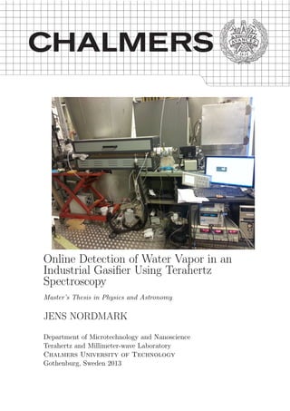
  • 1. Online Detection of Water Vapor in an Industrial Gasifier Using Terahertz Spectroscopy Master’s Thesis in Physics and Astronomy JENS NORDMARK Department of Microtechnology and Nanoscience Terahertz and Millimeter-wave Laboratory Chalmers University of Technology Gothenburg, Sweden 2013
  • 2. Online Detection of Water Vapor in an Industrial Gasifier Using Terahertz Spectroscopy Jens Nordmark c Jens Nordmark, 2013 Terahertz and millimeter wave laboratory Department of Microtechnology and Nanoscience Chalmers University of Technology SE-412 96 Gothenburg Sweden
  • 3. Abstract A terahertz spectrometer was set up for the monitoring of product gas in a thermal gasi- fier. The goal was to measure temperature and H2O concentration, and preferably also CO concentration. This environment presents several difficulties such as high tempera- ture, toxic gases, high H2O content and a high concentration of particulate pollutants. Spectroscopy using IR Lasers tend to be obstructed by the high absorption of H2O as well as the scattering by the particulates, and so does not produce satisfactory results. It was hoped that these problems could be avoided by using terahertz radiation, with a lower absorption by water and a longer wavelength possibly avoiding scattering by particulates. A system operating in the range 300-500 GHz was built and tested in lab- oratory as well as in an industrial gasifier at Chalmers Power center, yielding promising results. Our results indicate that monitoring of H2O, and probably other gases, in the rugged environment of gasifier rawgas can be done with response times on the order of a few minutes. This has applications in biomass gasification, where variable quality of the fuel results in a need for continous monitoring and tuning of the gasification process. Keywords: Terahertz, Gas spectroscopy, Gasification
  • 4.
  • 5. Acknowledgements I wish to thank my supervisor Sergey Cherednichenko for his help. I also wish to thank Hosein Bidgoli and Martin Seeman at the department for energy and the environment with whom the project was carried out. Also thanks to Johannes ¨Ohlin for assistance during experiments at the Chalmers power center. Jens Nordmark, Gothenburg July 1, 2013
  • 6.
  • 7. Contents Contents i List of Tables iv List of Figures vi Nomenclature x 1 Introduction 1 1.1 Data . . . . . . . . . . . . . . . . . . . . . . . . . . . . . . . . . . . . . . . 4 2 Theory 5 2.1 Gasification of biomass . . . . . . . . . . . . . . . . . . . . . . . . . . . . . 5 2.2 Terahertz technology . . . . . . . . . . . . . . . . . . . . . . . . . . . . . . 9 2.2.1 H2O and CO absorption at Terahertz frequencies . . . . . . . . . . 9 2.2.2 Detectors and sources . . . . . . . . . . . . . . . . . . . . . . . . . 11 2.2.3 Waveguides . . . . . . . . . . . . . . . . . . . . . . . . . . . . . . . 13 2.3 Molecular spectroscopy . . . . . . . . . . . . . . . . . . . . . . . . . . . . . 14 2.3.1 Energy levels . . . . . . . . . . . . . . . . . . . . . . . . . . . . . . 14 The vibration-rotation spectrum of CO . . . . . . . . . . . . . . . 15 2.3.2 Line shape . . . . . . . . . . . . . . . . . . . . . . . . . . . . . . . 16 Natural broadening . . . . . . . . . . . . . . . . . . . . . . . . . . . 17 Doppler broadening . . . . . . . . . . . . . . . . . . . . . . . . . . 17 Collisional broadening . . . . . . . . . . . . . . . . . . . . . . . . . 17 Combined broadening . . . . . . . . . . . . . . . . . . . . . . . . . 17 Temperature dependence of line strength . . . . . . . . . . . . . . 18 Line-by-line models . . . . . . . . . . . . . . . . . . . . . . . . . . . 18 2.3.3 Collisional line mixing . . . . . . . . . . . . . . . . . . . . . . . . . 18 2.3.4 The HITRAN database . . . . . . . . . . . . . . . . . . . . . . . . 19 i
  • 8. CONTENTS 2.3.5 LINEPAK vs custom algorithm . . . . . . . . . . . . . . . . . . . . 19 3 The setup 20 3.1 Gas cell design . . . . . . . . . . . . . . . . . . . . . . . . . . . . . . . . . 20 3.1.1 Window properties . . . . . . . . . . . . . . . . . . . . . . . . . . . 24 3.2 Spectrometer . . . . . . . . . . . . . . . . . . . . . . . . . . . . . . . . . . 26 3.2.1 Source . . . . . . . . . . . . . . . . . . . . . . . . . . . . . . . . . . 26 3.2.2 Detector: Golay cell . . . . . . . . . . . . . . . . . . . . . . . . . . 29 3.3 Humidity meter . . . . . . . . . . . . . . . . . . . . . . . . . . . . . . . . . 31 3.4 Spectrum analysis . . . . . . . . . . . . . . . . . . . . . . . . . . . . . . . 32 3.4.1 THz absorption by H2O vapors . . . . . . . . . . . . . . . . . . . . 32 3.4.2 THz absorption by Carbon Monoxide . . . . . . . . . . . . . . . . 32 4 Experimental methodology 35 4.1 Calibration . . . . . . . . . . . . . . . . . . . . . . . . . . . . . . . . . . . 35 4.2 Laboratory H2O measurements . . . . . . . . . . . . . . . . . . . . . . . . 37 4.3 Monitoring of H2O and CO at the gasifier . . . . . . . . . . . . . . . . . . 40 4.4 Noise and drifts . . . . . . . . . . . . . . . . . . . . . . . . . . . . . . . . . 44 5 Discussion 48 5.1 Detection of H2O . . . . . . . . . . . . . . . . . . . . . . . . . . . . . . . . 48 5.2 Detection of CO . . . . . . . . . . . . . . . . . . . . . . . . . . . . . . . . 51 5.3 Noise and drifts . . . . . . . . . . . . . . . . . . . . . . . . . . . . . . . . . 51 5.4 Other issues . . . . . . . . . . . . . . . . . . . . . . . . . . . . . . . . . . . 54 5.4.1 Temperature gradient and thermocouples . . . . . . . . . . . . . . 54 5.4.2 Line-by-line model vs LINEPAK . . . . . . . . . . . . . . . . . . . 54 5.5 Usability of the system . . . . . . . . . . . . . . . . . . . . . . . . . . . . . 54 Bibliography 57 A Line-by-line algortihm 60 B Line data from HITRAN2008 62 C SpectralCalc simulations 64 D Calculations of T and V MR from S380 and S448 70 D.1 Determination of T from measured V MR and S . . . . . . . . . . . . . . 70 ii
  • 9. CONTENTS D.2 Determination of V MR from calculated T and measured S . . . . . . . . 72 D.3 Simultaneous determination of T and V MR from S . . . . . . . . . . . . 73 E Humidity control 75 F Alternative waveguides 76 Index 77 iii
  • 10. List of Tables 2.1 The expected contents of gasifier rawgas at Chalmers power center, based on gas chromatography and H2O separation by condensation. All V MR entries except H2O refer to dry gas composition. (Hosein Bidgoli, private communication) . . . . . . . . . . . . . . . . . . . . . . . . . . . . . . . . . 6 2.2 The expected contents of gasifier fluegas at Chalmers power center, based on gas chromatography and H2O separation by condensation. All V MR entries except H2O refer to dry gas composition. (Hosein Bidgoli, private communication) . . . . . . . . . . . . . . . . . . . . . . . . . . . . . . . . . 6 2.3 Detector types for far IR and THz. A summary of Rogalski and Sizov [2011] 12 2.4 Sensitivity for some detector types for far IR and THz. A summary of Rogalski and Sizov [2011], last entry is a bolometer made at TML, MC2, Chalmers. Described in Cherednichenko et al. [2011]. . . . . . . . . . . . . 12 3.1 Amplitudes of frequency swings due to modulation with various ampli- tudes. ∆fin is the maximum deviation from the mean frequency at any particular value of the control voltage Uctrl, and is due to the value of the FM voltage UFM. ∆fout is the output frequency of the AMC after multiplication. The relation between FM modulation voltage and output frequency swing varies slightly across the operating range of our source, as can be seen in the difference in output from these two control voltages when all other parameters are kept constant. . . . . . . . . . . . . . . . . 27 3.2 Coefficients for the Antoine equation for H2O, from DDBST [2013]. . . . 31 4.1 Transmissions obtained at different humidity levels in two separate mea- surements of the type shown in figure 4.2. Errors are shown as one stan- dard deviation. Measurement number indicates which of the two separate dataseries the entry comes from. . . . . . . . . . . . . . . . . . . . . . . . 37 iv
  • 11. LIST OF TABLES 5.1 Temperature estimations using least-squares from the data in table 4.1. The calculation is shown in appendix D. Errors are given as one standard deviation. The last column shows how V MR is calculated assuming the calculated temperature and measured transmissions. . . . . . . . . . . . . 50 5.2 The result when fitting both T and V MR using the program in appendix D.3, and the same data as in the table above. . . . . . . . . . . . . . . . . 50 B.1 Spectral lines of CO . . . . . . . . . . . . . . . . . . . . . . . . . . . . . . 62 B.2 Spectral lines of water . . . . . . . . . . . . . . . . . . . . . . . . . . . . . 63 F.1 Transmission at three distances with and without waveguide, normalized to the 10 cm air transmission. . . . . . . . . . . . . . . . . . . . . . . . . . 76 v
  • 12. List of Figures 1.1 Scattering cross-section as function of frel = R/λ for a spherical particle. Calculated with MiePlot 4.3 by Laven [2013], implementing the BHMIE algorithm by Bohren and Huffman [2007]. [data/mie] . . . . . . . . . . . . 2 1.2 The spectra of two gas mixtures at room temperature (296 K). 10% H2O (blue) and 10% H2O+10% CO (red). [data/introspectrum] . . . . . . . . 2 1.3 The simulated spectra of H2O at V MR = 20% and varying temperatures. [data/AppendixC] . . . . . . . . . . . . . . . . . . . . . . . . . . . . . . . 3 1.4 The simulated spectra of H2O at T = 573K and varying humidity. [data/AppendixC] 3 2.1 The device measuring H2O content by condensation. H2O and tar con- dense while bubbling up from the bottom of the isopropanol pool, and mix with the liquid. The mass increase of the isopropanol container gives the amount of H2O and tar in a volume of gas, ∆m = mH2O + mtar. To give a good accuracy, the mass increase must be measured over periods of several hours. . . . . . . . . . . . . . . . . . . . . . . . . . . . . . . . . 6 2.2 The operating principle of the Chalmers gasifier . . . . . . . . . . . . . . . 8 2.3 Top: Spectra of 10% H2O and 10% CO + 10% H2O in the range 100GHz to 1 THz at 296 K. Bottom: The same restricted to 300-500 GHz. [data/simulation full] . . . . . . . . . . . . . . . . . . . . . . . . . . . . . . . . . . . . . . . 10 2.4 vibrational modes and rotational axes of CO and H2O . . . . . . . . . . . 15 2.5 Sketch of typical rovibrational spectrum for a diatomic molecule with a vibrational transition at 1000, and rotational constant of 1/2, in arbitrary units. . . . . . . . . . . . . . . . . . . . . . . . . . . . . . . . . . . . . . . 16 2.6 The type of transitions giving rise to line mixing. . . . . . . . . . . . . . . 19 3.1 A sketch of the gas cell . . . . . . . . . . . . . . . . . . . . . . . . . . . . . 21 3.2 The gas cell and its connections to the rest of the system. . . . . . . . . . 21 3.3 The gas cell set up at the gasifier . . . . . . . . . . . . . . . . . . . . . . . 22 3.4 The gas cell in the lab within the closed oven, tubing and electronics. . . 22 3.5 The gas cell inside the open oven . . . . . . . . . . . . . . . . . . . . . . . 23 vi
  • 13. LIST OF FIGURES 3.6 Transmission through teflon(top) and quartz(bottom) windows at normal incidence relative to air. [data/windowproperties/] . . . . . . . . . . . . . 25 3.7 The setup of the instruments around the gas cell . . . . . . . . . . . . . . 26 3.8 A nitrogen spectrum in terms of control voltage vs output voltage from the Golay cell. The voltage span corresponds to a full frequency sweep over 300-500 GHz. Note the very high sensitivity to small variations in the contol voltage. This sensitivity motivated the use of frequency modulation. [data/ctrl-to-signal] . . . . . . . . . . . . . . . . . . . . . . . 27 3.9 Sketch of the setup of the source, from VDI manual. . . . . . . . . . . . . 28 3.10 Source power output, from VDI manual. . . . . . . . . . . . . . . . . . . . 28 3.11 Sketch of the Golay cell . . . . . . . . . . . . . . . . . . . . . . . . . . . . 29 3.12 Left: Golay cell. Right: The microwave source . . . . . . . . . . . . . . . 30 3.13 The Amplifier multiplier chain, concealed within a black box. . . . . . . . 30 3.14 Line positions and intensities for H2O. Upper left: 0-40 cm−1 with cutoff at intensity < e−23. Upper right: 0-40 cm−1 with no cutoff. Lower left: 10-16.7 cm−1 with cutoff at intensity < e−23 Lower right: 10-16.7 cm−1 with no cutoff. Compare figure 2.3. . . . . . . . . . . . . . . . . . . . . . . 33 3.15 Line positions and intensities for CO. Upper left: 0-40 cm−1 with cutoff at intensity < e−23. Upper right: 0-40 cm−1 with no cutoff. Lower left: 10-16.7 cm−1 with cutoff at intensity < e−23 Lower right: 10-16.7 cm−1 with no cutoff. Compare figure 2.3. . . . . . . . . . . . . . . . . . . . . . . 34 4.1 Top: Two raw measurements, one of N2 which lacks spectral lines in this frequency range to be used for calibration, and one of gasifier rawgas. Bot- tom: The transmission spectrum formed by dividing the rawgasspectra by the calibration spectra. V MR ≈ 65% and T ≈ 430oC. [data/rawspectra] 36 4.2 Top: the two water lines are plotted as functions of time, where the H2O content is changed in steps. Bottom: the humidity meter gives the corresponding V MR. [data/twolines] . . . . . . . . . . . . . . . . . . . . . 38 4.3 Laboratory measurement of transmission at 449 GHz over time for five humidity levels. The impulse-like objects are products of the humidifier, it seems to release steam in short pulses. Note that measurements with a difference in V MR as small as 0.4% can be clearly distinguished from each other. [/data/20130204] . . . . . . . . . . . . . . . . . . . . . . . . . 39 4.4 The spectrum of the rawgas, 300-500 GHz. Note the CO line at 460 GHz. Also included is a fluegas measurement at 410-470 GHz. Spectralcalc simulations for the rawgas are also included, compare table 2.1 of rawgas contents. [data/rawgasplot] . . . . . . . . . . . . . . . . . . . . . . . . . . 41 4.5 Raw and fluegas from the same measurement as above, zoomed in on the H2O-line at 448 GHz.[data/rawgasplot] . . . . . . . . . . . . . . . . . . . 41 4.6 H2O (41%) compared to H2O (41%) and CO (20%). [/data/coandh2o] . 42 vii
  • 14. LIST OF FIGURES 4.7 Measurement over time of the 448 GHz transmission at the gasifier. Vary- ing the steam input of the process: 160, 200, 240, 160, 120 kg/h. [data/gasifier- humiditylevels] . . . . . . . . . . . . . . . . . . . . . . . . . . . . . . . . . 43 4.8 N2 spectra taken over a period of four hours for the gas cell at room temperature and normalized to the first one of them. Moving average over 15 GHz.[data/drifts/book3-20130311] . . . . . . . . . . . . . . . . . . 45 4.9 N2 spectra taken over a period of eight hours at high temperature (oven at 600 C) and normalized to the first one of them. The legend shows the time that the corresponding measurement was taken. Moving average over 15 GHz.[data/drifts/book1-20130312] . . . . . . . . . . . . . . . . . . 46 4.10 N2 spectra taken over a period of five hours at high temperature (oven at 600 C) and normalized to the first one of them, with better thermal isolation (10 cm more air between source and gas cell) than in figure 4.9. Moving average over 15 GHz.[data/drifts/book2-20130327] . . . . . . . . . 46 4.11 Noise plot in the lab obtained by division of two subsequent N2-spectra. Integration time 100 ms. Note that signal strength approaches zero at the ends of the spectrum, causing signal-to-noise ratio to decrease. In this plot no smoothing has been used. [data/noise] . . . . . . . . . . . . . 47 4.12 Noise plot at the gasifier obtained by division of two subsequent N2- spectra. Integration time 100 ms. In this plot no smoothing has been used. [data/noise] . . . . . . . . . . . . . . . . . . . . . . . . . . . . . . . . 47 5.1 Transmission as function of temperature calculated by the line-by-line- model for the V MR of 73% detected in the measurements of figure . The black lines show where the measured transmissions intersect the simula- tion, giving the temperature. The values of T should coincide, but do not. Precise estimates from a least-squares fit for several measurements of this type are shown in table 5.1. [data/temp humidity] . . . . . . . . . . . . . 49 5.2 Transmission as function of temperature calculated by Spectralcalc for the V MR of 73% detected in the measurements of figure . The black lines show where the measured transmissions intersect the simulation, giving the temperature. The values of T should coincide, but do not. The temperatures differ much more than above. [data/temp humidity] . . . . 49 5.3 An N2 measurement at 383 GHz with 300 millisecond integration time and one data point taken per second, in the lab.[data/rmsd] . . . . . . . . 52 5.4 Allan variance of the above signal.[data/rmsd] . . . . . . . . . . . . . . . . 52 5.5 The 449 GHz line from rawgas at the gasifier (200 kg/h of H2O), mon- itored for 1200 seconds. 100 millisecond integration time and one data point taken per 300 milliseconds.[data/rmsd] . . . . . . . . . . . . . . . . 53 5.6 Allan variance of the above signal. [data/rmsd] . . . . . . . . . . . . . . . 53 5.7 A comparison of rawgas measurment, spectralcalc and line-by-line simu- lation. [data/comparison] . . . . . . . . . . . . . . . . . . . . . . . . . . . 55 viii
  • 15. LIST OF FIGURES C.1 The simulated spectra of H2O at V MR = 20% and varying temperatures. [data/AppendixC] . . . . . . . . . . . . . . . . . . . . . . . . . . . . . . . 65 C.2 The simulated spectra of H2O at T = 573K and varying humidity. [data/AppendixC] 65 C.3 Ratio of H2O peak transmission at 448 and 383 as function of temperature when V MR is kept constant at 20%. [data/AppendixC] . . . . . . . . . . 66 C.4 Ratio of H2O peak transmission at 448 and 383 as function of V MR when T is kept constant at 573 K. [data/AppendixC] . . . . . . . . . . . . . . . 66 C.5 The simulated transmission of H2O at 380 GHz for various T and V MR. [data/AppendixC] . . . . . . . . . . . . . . . . . . . . . . . . . . . . . . . 67 C.6 The simulated transmission of H2O at 448 GHz for various T and V MR. [data/AppendixC] . . . . . . . . . . . . . . . . . . . . . . . . . . . . . . . 67 C.7 The simulated transmission at 380 GHz, dependence on T for 10 different values of H2O V MR. [data/AppendixC] . . . . . . . . . . . . . . . . . . . 68 C.8 The simulated transmission at 448 GHz, dependence on T for 10 different values of H2O V MR. [data/AppendixC] . . . . . . . . . . . . . . . . . . . 68 C.9 The simulated transmission at 380 GHz, dependence on H2O V MR for 12 different values of T. [data/AppendixC] . . . . . . . . . . . . . . . . . 69 C.10 The simulated transmission at 448 GHz, dependence on H2O V MR for 12 different values of T. [data/AppendixC] . . . . . . . . . . . . . . . . . 69 ix
  • 16. Nomenclature CH4 Methane CO Carbon monoxide CO2 Carbon dioxide H2 Hydrogen RH Relative Humidity, ratio of H2O partial pressure to saturated vapor pressure. V MR Volume Mixing Ratio AMC Amplifier-/Multiplier Chain EM Electromagnetism, Electromagnetic GPIB General purpose interface bus, same as IEEE 488 HITRAN high-resolution transmission molecular absorption database IEEE Institute of Electrical and Electronics Engineers IEEE 488 General purpose interface bus, GPIB IR Infrared LINEPAK Software library for spectral simulation described in Gordley et al. [1994]. NEP Noise Equivalent Power RMSD Root Mean Square Deviation SNG Substitute Natural Gas, methane tar A loosely defined viscous black substance consisting mainly of large hydrocarbons, often aromatic, polycyclic and containing various sub- stituents. THz TeraHertz TTL Transistor-Transistor Logic, a binary logic scheme using 0-0.8 V signals for low and 2.2-5 V for high x
  • 17. 1 Introduction Gasification of biomass is a technology expected to become more important as fossil fuels are to be replaced by carbon neutral bioenergy. The company WSP has made projections based on three scenarios, showing a potential for up to 12 TWh in biogas production by thermal gasification up to 2030 under favorable conditions. Distribution of the combustible gas produced (typically SNG, i.e. methane) could take place using the present natural gas infrastructure (Dahlgren et al. [2013]). The properties of the fuels used are however such that the producer gas, also called rawgas in the stage immediately after it is generated, is full of char particles at sizes up to about one micron. At the same time its gas contents vary in time, and need to be tracked to tune the process. The particulate contents as well as the high H2O content disturb the IR-spectroscopy that would typically be used to monitor gas content. H2O simply has to high absorption in the IR for such radiation to be used successfully. The wavelength of IR is also at the order of the particulates diameter, giving rise to scatter- ing that disrupts measurements. Gas chromatography is another technique traditionally used, but it cannot handle gas mixtures containing H2O, which condenses in the chro- matograph and destroys it. It is possible to measure the dry gas composition by first drying and cleaning the gas. This also provides a way to determine the sum of H2O and tar contents, but only the total content and not both independently. In addition, it only works with a time delay of tens of minutes. As an alternative solution, this project aimed to use terahertz spectroscopy in the hope to escape the aforementioned problems. Our aim was to measure content of H2O as well as CO, one of the dry gases present. Our results indicate that this approach does work as desired. There are several reasons why this approach succeeds. THz has a lower absorption for H2O, avoiding saturation of the spectral lines. THz has longer wavelengths than IR, which reduces the scattering by particulates. The scattering of radiation by ideal spherical particles is described by Mie theory, where a threshold in the scattering cross 1
  • 18. CHAPTER 1. INTRODUCTION 1.00EͲ11 1.00EͲ09 1.00EͲ07 1.00EͲ05 1.00EͲ03 1.00EͲ01 1.00E+01 1.00E+03 0 0.5 1 1.5 2 2.5 3 Cross section Scatterer size (Radius/wavelength) Figure 1.1: Scattering cross-section as function of frel = R/λ for a spherical particle. Calculated with MiePlot 4.3 by Laven [2013], implementing the BHMIE algorithm by Bohren and Huffman [2007]. [data/mie] 0.5 0.6 0.7 0.8 0.9 1 300 320 340 360 380 400 420 440 460 480 500 Transmission Frequency [GHz] H2O+CO H2O Figure 1.2: The spectra of two gas mixtures at room temperature (296 K). 10% H2O (blue) and 10% H2O+10% CO (red). [data/introspectrum] section appears when the wavelength is comparable to the size of the scatterers, which can be formulated in terms of the relative frequency frel = R/λ ≈ 1/2 as shown in figure 1.1. In the low frequency limit, there is weak Rayleigh scattering that decreases quickly with particle size, while in the optical limit of large frel the scattering cross section is close to 1. By increasing λ we decrease relative frequency (frel) and thus move closer to the Rayleigh limit. This was one of the motivations for using THz radiation. Spectroscopy in field environments using terahertz has been demonstrated in several applications, for instance the remote detection of chemicals in Gopalsami et al. [2008] or the remote detection of nuclear radiation in Gopalsami et al. [2009]. Currently the spectra of H2O as well as that of CO in the region 300-500 GHz are well known and included in the HITRAN database. This spectral range contains a few strong H2O lines and a few conveniently places CO lines, shown in figure 1.2. The absorption at the line centers is dependent on both concentration and tem- 2
  • 19. CHAPTER 1. INTRODUCTION perature as shown in figures 1.3 and 1.4. Thus it is possible to determine these two parameters from measured spectra. Figure 1.3: The simulated spectra of H2O at V MR = 20% and varying temperatures. [data/AppendixC] Figure 1.4: The simulated spectra of H2O at T = 573K and varying humidity. [data/AppendixC] 3
  • 20. 1.1. DATA CHAPTER 1. INTRODUCTION 1.1 Data Some of the data and code used for obtaining the figures in the text has been put in the following Google Drive folder: https://drive.google.com/folderview?id=0B25vmzARFvvOdnlYNDBocEFQNGM 4
  • 21. 2 Theory 2.1 Gasification of biomass Production of combustible gas from biomass can be achieved using several processess, including biological and thermal. In the present project, we are concerned with thermal gasification of biomass, particularly from wood pellets. However, many types of high- grade biomass are required in other industries and the energy sector will have to settle for the leftovers. Thus it will be necessary to handle a highly variable input in a process. This is why online detection of the product is required, since the process must be continuosly tuned to the variable input. In thermal gasification the solid biomass is broken down thermally in the presence of an oxidising agent, in this case H2O. The main products are CO, CO2, H2, CH4, tars and other hydrocarbons. The dry gases and the water contents expected in the rawgas of the Chalmers gasifier are given in table 2.1, and for the fluegas data are given in table 2.2. Primary tars are of the form CxHyOz, but are themselves broken down into either new tars, H2 or the product gases mentioned. The process requires a temperature above 600oC. (Gomez-Barea and Leckner [2010]). The H2O content is of critical importance in regulating the rate of the process, since it is involved in most reactions breaking down the large molecules of the fuel into product gas. The contents of the gas must be very finely tuned for downstream processes to work, which requires a low-delay monitoring of the most significant species. The intended downstream process in this case is generation of substitute natural gas (SNG), by the process of water gas shift: 3H2 + CO → CH4 + H2O (2.1) This is highly sensitive to the ratio of CO to H2. 5
  • 22. 2.1. GASIFICATION OF BIOMASS CHAPTER 2. THEORY Table 2.1: The expected contents of gasifier rawgas at Chalmers power center, based on gas chromatography and H2O separation by condensation. All V MR entries except H2O refer to dry gas composition. (Hosein Bidgoli, private communication) Gas H2 CO CO2 CH4 C2H2 C2H4 V MR [%] 4.64 23.40 35.50 16.35 13.78 0.33 Gas (cont.) C2H6 C3H6 C3H8 He N2 H2O V MR [%] 0.70 0.47 0.02 1.11 3.42 ca 65 Table 2.2: The expected contents of gasifier fluegas at Chalmers power center, based on gas chromatography and H2O separation by condensation. All V MR entries except H2O refer to dry gas composition. (Hosein Bidgoli, private communication) Gas N2 O2 CO2 H2O V MR [%] 79.5 3.5 17 ca 20 Figure 2.1: The device measuring H2O content by condensation. H2O and tar condense while bubbling up from the bottom of the isopropanol pool, and mix with the liquid. The mass increase of the isopropanol container gives the amount of H2O and tar in a volume of gas, ∆m = mH2O + mtar. To give a good accuracy, the mass increase must be measured over periods of several hours. 6
  • 23. 2.1. GASIFICATION OF BIOMASS CHAPTER 2. THEORY Other methods than THz spectroscopy to monitor H2O are IR spectroscopy or con- densation (explained in figure 2.1). IR spectroscopy has the problems of increased scat- tering by the particulates, due to the shorter wavelength of IR compared to terahertz. The absorption of water is also very high in the IR, creating a risk of saturation of such spectrometers. Condensation is more robust: just let the H2O condense and compare its mass to the volume of gas it came from. But this creates a long delay and also fails to differentiate between H2O and tar, since tar also condenses. This motivates the attempt to use THz instead. A gasifier has a bed of material with high heat capacity to keep the fuel at an even temperature. There are several designs of these beds, in the Chalmers case it is a fluidized bed, made of sand that has properties resembling a fluid when under the conditions of the gasifiers operation. The fuel is mixed with the bed material. Heat is provided by a separate combustion chamber, this is called external heating to differentiate from the case where the gasifier itself provides heat. Bed material is continously circulated between combustion chamber and gasifier to provide heat. Bubbles of steam will move upward through the bed material, accumulating gasifier products along the way. At this stage the particulates in the gas are small, submicron size, so they will not affect the THz radiation much. The temperature of flue- and rawgas leaving the gasifier is anticipated to be around 850o C, which is the operating temperature of the process, but it cools down to about 350o C before reaching the gas cell, since it is transported in heating hoses with a capacity of maximum 350o C. It is then heated again inside the oven to 430o C to avoid condensation in the gas cell. Figure 2.2 shows a flow diagram of the process at the Chalmers gasifier. Fuel is fed from above into both chambers. In the combustion chamber, air is injected for combustion while in the gasification chamber steam, the oxidizing agent, is inserted instead. Heat is transported from the combustion chamber to the gasification chamber by circulation of the hot sand of the fluidized bed. The output gas of the combustor is referred to as fluegas, while the product gas of the gasifier is called rawgas when it is leaving the gasifier, before being cleaned for downstream use. 7
  • 24. 2.1. GASIFICATION OF BIOMASS CHAPTER 2. THEORY Figure 2.2: The operating principle of the Chalmers gasifier 8
  • 25. 2.2. TERAHERTZ TECHNOLOGY CHAPTER 2. THEORY 2.2 Terahertz technology The terahertz region of the electromagnetic spectrum is defined as wavelengths from 3mm to 30 µm. It starts at the upper edge of millimeter waves and ends at the lower edge of the infrared. Generation and detection of radiation in this range is more difficult than in the microwave region of the EM spectrum, and THz equipment is currently an area of intense research. Several applications of THz radiation exploit its ability to penetrate tissue, fabric and plastics to a significant depth, while being partially reflected depending on density and contents of objects. This makes possible a variety of imaging applications. In addition, it is non-ionizing1 and thus harmless to living organisms unless used with very high power output, which tends to be neither needed nor available. In the present project, we attempted to exploit THz radiation in the monitoring of water vapor content in dirty gasifier rawgas, where IR laser spectroscopy fails due to the particulate matter in the gas. THz was expected to pass through the particulates. We also face the issue of high temperatures. Temperature affects spectral lines both by changing their relative strengths and by broadening of lines. This is further described in section 2.3.2. 2.2.1 H2O and CO absorption at Terahertz frequencies We need to detect H2O under various concentrations and temperatures. It is important to avoid saturation of the spectrometer. In figure 2.3 we show the spectra of H2O as well as CO. Three of the H2O lines are very strong and risk to saturate our system. We want several weak lines in the frequency range used. The band 300-500 GHz suits this purpose for both gases considered, and equipment for sweeping over these frequencies exists. The danger of saturation is exacerbated by high temperatures, which increase absorption significantly. See appendix C for plots of the temperature dependence of absorption at various concentrations of H2O. 1 Photon energies vary from 0.413 meV at 3 mm to 41.3 meV av 30 µm 9
  • 26. 2.2. TERAHERTZ TECHNOLOGY CHAPTER 2. THEORY 0 0.1 0.2 0.3 0.4 0.5 0.6 0.7 0.8 0.9 1 1002003004005006007008009001000 Transmission Frequency [GHz] H2O+CO H2O 0.9 0.91 0.92 0.93 0.94 0.95 0.96 0.97 0.98 0.99 1 300320340360380400420440460480500 Transmission Frequency [GHz] H2O+CO H2O Figure2.3:Top:Spectraof10%H2Oand10%CO+10%H2Ointherange100GHzto1THzat296K.Bottom:Thesame restrictedto300-500GHz.[data/simulationfull] 10
  • 27. 2.2. TERAHERTZ TECHNOLOGY CHAPTER 2. THEORY 2.2.2 Detectors and sources Detectors for THz can be broadly categorized into thermal or photon detectors, as Ro- galski and Sizov [2011] describe. Thermal detectors absorb the radiation and gain heat, which induces change in some physical property of the material that can be easily mea- sured. For instance, metals or semiconductors can be used that change their electrical conductivity in response to temperature differences. This is a common category of de- tectors called Bolometers. Another example would be to measure the thermal expansion of a gas, which is the method we use. That type of detector is called a Golay cell and is described in detail in section 3.2.2. Thermocouples are devices that generate voltage over a junction of two different materials in response to temperature changes. They are used in many applications and can be used as IR detectors as well as for temperature measurements in general. Photon detectors rely on excitations in semiconductors. When a photon is absorbed its energy gives rise to an electron-hole pair. These gives rise to electrical conduction, in a variety of ways for different detector types. They have a frequency-dependent response, unlike thermal detectors. Their advantage is that they tend to have very fast response times and good signal-to-noise ratio. A major inconvenience is that they require cooling to very low temperatures to avoid thermally generated noise. A thermal detector is for this reason the favoured option provided that its precision is acceptable. The Golay cell was used because it was available. We list some detector types in table 2.3. A measure of detector sensitivity in common use is Noise Equivalent Power, NEP. It is defined as the power required of an input signal to generate a signal-to-noise ratio of 1 in an output signal with 1 Hz bandwidth. The unit is W / √ Hz. This should of course be as low as possible for good detectors. A few examples from Rogalski and Sizov [2011] are collected in table 2.4. A higher sensitivty of a detector lessens the noise and shortens the required integration time at a particular noise level. 11
  • 28. 2.2. TERAHERTZ TECHNOLOGY CHAPTER 2. THEORY Table 2.3: Detector types for far IR and THz. A summary of Rogalski and Sizov [2011] Category Detector type Mechanism Thermal Bolometers Temperature dependence of conductivity Thermocouple Voltage generated by temperature change Pyroelectric Charged plane conductors changing polarity Golay cell Thermal expansion of gas Photon Photoconductors Photon absorption in energies above the band gap cre- ates carrier/hole pair in a uniform piece of some semi- conductor, raising conductivity. p-n junction diodes Photon-induced pair production creates a photocur- rent across a junction between p- and n-doped semi- conductors Schottky barrier diodes Photocurrent across Schottky barrier Table 2.4: Sensitivity for some detector types for far IR and THz. A summary of Rogalski and Sizov [2011], last entry is a bolometer made at TML, MC2, Chalmers. Described in Cherednichenko et al. [2011]. Detector type NEP [W / √ Hz] Golay cell 10−9 − 10−10 Schottky diode 10−10, increasing with ν Bi bolometer 1.6 × 10⁻¹⁰, increasing with ν Nb microbolometer 5 × 10⁻¹¹ Ti microbolometer 4 × 10⁻¹¹ Ni microbolometer 1.9 × 10⁻¹¹ YBCO bolometer 3.7 × 10⁻¹⁰ 12
  • 29. 2.2. TERAHERTZ TECHNOLOGY CHAPTER 2. THEORY 2.2.3 Waveguides Waveguides are conducting tubes used to transfer radiation with as little attenuation as possible. Their dimensions are chosen with respect to the wavelength of the radiation considered, and longer wavelengths require broader waveguides. Each waveguide geom- etry has a cutoff frequency below which decay of the transmitted wave will occur. All waveguides that are not perfect conductors will experience attenuation, which is lower for higher frequencies. The minimum attenuation naturally occurs for an infinitely large waveguide, but detector apertures tend to be quite small and one needs to balance these two requirements. Conical horns at the end of the waveguide is one way of balancing these needs. Waveguides at which the intended wavelength is small enough to allow ”overmoding”, where many additional modes of propagation can occur, are called over- sized waveguides. These give a low attenuation, but less mode purity. Such a waveguide was used in this project. It is oversized since it has an internal diameter of 26 mm while the longest wavelength used is 1 mm. In our case only the total transmitted energy is measured, the Golay cell treats all modes of propagation equally, so overmoding is not a big problem. 13
  • 30. 2.3. MOLECULAR SPECTROSCOPY CHAPTER 2. THEORY 2.3 Molecular spectroscopy When EM radiation passes through a sample, its rate of transmission will depend on various properties of the sample. The Beer-Lambert law formulates this as: T = T0e−Al (2.2) where l is the length of the sample along the beam and A is an absorption coefficient, de- pending of a number of parameters. Since these parameters are specific to the substances in a sample, as well as to some other conditions such as pressure and temperature, one can infer facts about the sample by studying its absorption spectrum. Calculating the absorption in relation to the pressure, temperature and composition is the subject of the following sections. 2.3.1 Energy levels In an atom there are only electronic energy levels, which usually have optical transitions. Some fine structure transitions are in the terahertz, though. When forming a molecule, valence electrons of the constituent atoms will inhabit molecular orbitals instead of the atomic orbitals, with somewhat different energies. But there are also new degrees of freedom present. Molecules do not have rotational symmetry and will thus have rotational energy. The rotation must be treated quantum mechanically by rewriting the expression for rotational energy with quantum mechanical operators, and this gives rise to quantized rotational states. This will be demonstrated for CO below. Each molecular bond will in addition introduce vibrational modes, giving a spectrum of vibrational states. The number of vibrational modes depends on the molecule. A diatomic molecule such as CO has only one vibrational mode, while water is more complicated and has three vibrational modes. A sketch of the various modes of the two molecules is given in figure 2.4. To calculate electronic energy levels in molecules one uses the Born-Oppenheimer approximation: nuclear and electronic motion are assumed to be completely separate. This is justified since electron mass is about two thousandths of the mass of a nucleon, thus moving much quicker. In effect, electron wavefunctions depend only on the position of the nuclei and the motion of the nuclei depends only on the time-averaged distribution of electrons. Another approximation that might be used is to consider the molecule a rigid rotor when calculating rotational energy levels. Without this assumption there is some vibration-rotation coupling. This is however true to a significant degree at higher energy levels and then the rigid rotor approximation has to be abandoned. Vibration can be modeled as a harmonic oscillator for low energy levels, but at high energy levels it must be replaced by an anharmonic oscillator that couples to the rotation. While rotation-vibration in diatomic molecules can be handled analytically with ease the difficulty increases enormously for even triatomic molecules such as water. Theses are written on this subject, for instance Lori [2008]. A basic description of the vibrational levels would be a linear superposition of single-mode vibrations, but calculating exact levels requires handling nonlinear effects. We instead describe the diatomic molecule. 14
  • 31. 2.3. MOLECULAR SPECTROSCOPY CHAPTER 2. THEORY Figure 2.4: vibrational modes and rotational axes of CO and H2O The vibration-rotation spectrum of CO Vibration of CO is modeled as a harmonic oscillator for low energy levels (McQuarrie [2008], chapter 5), so the energy levels are of the form Evib = (ν + 1 2)¯hω where ω = k µ is determined empirically. µ is the reduced mass and k is the bond force constant. These lines generally are in the infrared. For CO, ν = 1 → 2 is at 269 meV or 65 THz. Rotation of CO is modeled as a rigid rotor with length re, the interatomic distance at equilibrium. Its moment of inertia, with respect to a line normal to the bond and intersecting it at the center of mass, is then given by I = µr2 e where µ is the reduced mass of the two-body system. We can insert this in the Schr¨odinger equation expressed in terms of the angular momentum operator J: J2 2I ψ = Erotψ (2.3) with eigenvalues Erot = ¯h2 2I j(j +1). In the case of CO we do not have to worry about the other rotational axes, one is identical and the other is a symmetry axis. Inserting the parameters for CO (from Hush and Williams [1974]) gives Erot = 0.24j(j +1)meV . This 15
  • 32. 2.3. MOLECULAR SPECTROSCOPY CHAPTER 2. THEORY Figure 2.5: Sketch of typical rovibrational spectrum for a diatomic molecule with a vibra- tional transition at 1000, and rotational constant of 1/2, in arbitrary units. is a multiple of about 58 GHz, starting in the microwave region. It is not surprising that rotational lines are also present in the neighboring THz region. The energy of the tran- sitions has a clear hierarchy, electronic>vibrational>rotational. Rotiational transitions are on the order of 1-10 cm−1 compared to about 1000 cm−1 for vibrational transitions. For each vibrational level one can thus superimpose rotational transitions and get a spectrum such as that sketched in figure 2.5. Selection rule ∆J = 0 suppresses the pure vibrational transition, which is surrounded by two branches of rotational transitions, the lower energy P-branch for ∆J = −1 transitions and the higher energy R-branch of ∆J = 1. Similar principles apply for the water molecule, but the calculations are very involved. Both CO and H2O have rotational lines in the region 300-500 GHz, where we have measured. See figure 3.15 for the rotational lines of CO. They can be easily understood, while the H2O lines in figure 3.14 are more complex. In practical applications one uses semiempirical rather than calculated spectra. 2.3.2 Line shape The line shape is affected by pressure- and temperature induced broadening, tempera- ture dependences in line strength, and line mixing. There are three main types of line broadening (Liou [2002], chapter 1): • Natural broadening: due to the time-energy uncertainty principle. • Doppler broadening: due to doppler shifts of the radiation from sources moving in all directions. • Pressure broadening: due to several pressure-dependent effects including collisions (shortening excited state lifetimes) and perturbations of the energy levels of atoms by the electric fields of nearby atoms. We briefly describe these types to show which are important in our case. 16
  • 33. 2.3. MOLECULAR SPECTROSCOPY CHAPTER 2. THEORY Natural broadening This type of broadening is the most fundamental, existing due to the Heisenberg uncer- tainty principle: ∆E∆t ≥ h/2π (2.4) The lifetime of a state is thus inversely proportional to its uncertainty in energy. Unless states in the gas are extremely short-lived, this is completely negligible. Doppler broadening The velocity of molecules in a gas follow a Maxwell distribution: p(v) = 1 √ πv0 ev2/v0 (2.5) where v0 is the mean speed given by v0 = 2kBT/m. This gives rise to a Gaussian lineshape: fD(ν − ν0) = 1 αD √ π exp − (ν − ν0)2 α2 D (2.6) where αD = ν0 2kBT mc2 . This type of broadening is significant at very high temperatures or at low pressures, and the temperatures in our case might be high enough. Collisional broadening Collisional broadening follows a Lorentz line shape: f(ν − ν0) = α/π (ν − ν0)2 + α2 (2.7) where α = α0 p p0 T0 T n (2.8) Where α0 is the halfwidth at reference temperature T0. The half-width is composed of the self- and foreign-broadened halfwidths, that are added with weighting in accordance with the volume mixing ratio (V MR) of the gases present. This type of broadening is very significant in atmospheric pressures and temperatures, and in the temperature range we are to operate in. Combined broadening If more than one type of broadening is relevant the lineshape functions can be convoluted to get a realistic shape. When convoluting the Lorentz and Gaussian functions, one gets the Voigt function, a function for which there is no closed form expression. This could possibly improve our modelling algorithm. 17
  • 34. 2.3. MOLECULAR SPECTROSCOPY CHAPTER 2. THEORY Temperature dependence of line strength The line strength parameter Si(T) is necessary to determine the shape of the spectrum. It has a temperature dependence given by: S(T) = S(T0) e−hcEL/kBT QT (T0)[1 − e−hcν0/kBT ] e−hcEL/kBT0 QT (T)[1 − e−hcν0/kBT0 ] (2.9) where T0 is a reference temperature and T is the temperature considered. QT is the thermodynamic partition function and is specific to each chemical species. EL is the energy of the lower state in the transition and ν0 is the frequency of the line center. Line-by-line models To calculate the transmission profile one must sum the contribution of all nearby lines, one at a time. We describe how to do this in the most straightforward way, although highly optimized schemes exist for saving computational power. The direct approach is to calculate the contribution of each spectral line at each frequency and sum over all spectral lines in the vicinity of the spectral range of interest. The transmission at frequency ν can be written as T(ν) = i Si(T)f(ν − νi; αi)l (2.10) there T is total transmission, Si is line strength of line i, f is a shape function (Lorentz under atmospheric and similar condition), α is the Lorentz half-width and l is the length of the radiations passage through the medium. The α is itself affected by pressure, temperature and V MR of gases as described above. 2.3.3 Collisional line mixing An effect that is significant in IR gas spectroscopy is pressure-induced collisional mixing of lines. Adjacent lines will interfere with each other to a significant degree, which will create line profiles the differ significantly from the ones calculated by a line-by-line Lorentz-profile model. To see why this is so, we refer to a toy example by Hartmann et al. [2008], chapter four, pp. 148. The example assumes we have a pair of transitions i → f and i → f , both in the optical range. If the transitions i → i or f → f are very small, they might be triggered by collision, thus introducing processes such as i → i → f that mix the two optical lines. An illustration is shown in figure 2.6. While we obviously don’t get mixing between optical states of different molecules, the lineshapes of a molecule will still be affected by molecules of other species as well as its own kind. This is due to the low energy transitions triggered in the collisions, that transfer energy from one molecule to another in a way that is specific for each pair of molecules. To calculate the effects of line mixing one thus needs calculated or empirical mixing coefficients for each combination of gases. There is a large number of models for handling line mixing with varying precision and computational complexity, from simple classical models to full quantum scattering models. 18
  • 35. 2.3. MOLECULAR SPECTROSCOPY CHAPTER 2. THEORY Collisional transition Collisional transition Optical transitions E Figure 2.6: The type of transitions giving rise to line mixing. 2.3.4 The HITRAN database The HITRAN (high-resolution transmission molecular absorption) database contains empirical data on a large number of spectral lines for a number of molecules, including CO and H2O. It contains intensities and positions as well as lineshape parameters over a wide range of frequencies. The foreign-broadened halfwidths are given with respect to air. The database contents as of 2008 are described by Rothman et al. [2009]. 2.3.5 LINEPAK vs custom algorithm Since the effects described above are quite complex to simulate, much work has been done by researchers on optimizing algorithms for this task. In this project we used the webservice SpectralCalc, provided by GATS, Inc and powered by the LINEPAK library of GATS founder L. Gordley, described in Gordley et al. [1994]. The simulation takes all of the effects mentioned above into account and automatically collects needed data from HITRAN. It proved less tedious to extrapolate from a dataset obtained using Spectral- Calc rather than perfecting a custom algorithm for spectral simulation. The primary difficulty in simulating spectra in the range considered in this project is the complexity of line mixing, which is very significant for H2O. The line-by-line Lorentz-profile algorithm is included in appendix A. The dataset downloaded from Spectralcalc.com is described in appendix C. 19
  • 36. 3 The setup 3.1 Gas cell design The gas cell was a sealed steel tube (with inner diamter 26 mm and outer diameter 33 mm) with dual windows at both ends. The compartment for the sample gas was 1 m long, and in total the tube was 1.8 m long. The inner windows were made of crystalline quartz, 5mm thick, and the outer ones were made of teflon, 2mm thick. Both window materials are mostly transparent in the frequency range used, the transmission as function of frequency is plotted in figure 3.6. The windows where inserted at a 60o angle to the beam to minimize standing waves and other unwanted reflections. The gas cell was fully enclosed, except for the ends, by an oven (Entech ESTF 50/11-11) to keep the temperature stable. A sketch of the cell is shown in figure 3.1 and its connections to the other system components is shown in figure 3.2. A photo of the gas cell is shown in figure 3.5. In the laboratory setting, nitrogen gas was injected at a rate of 5L/min using a Bronkhorst EL-FLOW mass flow controller, and pre-heated using heating hoses from Hillesheim, model H3406-030-08-250C-83 and temperature controllers HT-40. Steam was injected into the nitrogen stream before entering the gas cell, using a steam genera- tor from Cellkraft (E-1000 precision evaporator). The gas flowed continuously through the gas cell and exited at the opposite end into the open air. Thus a temperature gra- dient formed when equilibrium was reached, and this was approximately measured with thermocouples at inlet and outlet. Figure 3.4 shows a photo of the setup. The volume between the windows was continously flushed with N2, with mass flow controllers set to 1 L/min, to avoid contamination with H2O or other gases. In the gasifier setting, the input rawgas came directly from the gasifier, and exited into the gas cleaning apparatus of the facility. Fluegas was also measured, directly from the combustor. Several times the input gas was also switched to bottle gas for testing of CO detection. Figure 3.3 shows a photo of the setup. 20
  • 37. 3.1. GAS CELL DESIGN CHAPTER 3. THE SETUP Gas inlet Gas outlet + thermocouple insertion N2 N2 Heating zone 1 Heating zone 1 Heating zone 2 Heating zone 2 Gas pre-heating Thermocouple insertion 1.0m 1.8 m 33mm 26mm W1 W1W2 W2 W1: Teflon windows W2: Quartz windows Figure 3.1: A sketch of the gas cell Water Humidity meter Heating hoses 200 C Steam generator Cellkraft E-1000 Precision Evaporator Into open air Mass flow controllers Bronkhorst EL-FLOW 1 L/min 1 L/min 5 L/min N2 wall outlet 7 atm Digital scale Ohaus Scout Pro Gas inlet Gas outlet N2 N2 Gas pre-heating Oven Entech ESTF 50/11-11 Thermocouple Thermocouple Hillesheim H3406-030-08-250C-83 Figure 3.2: The gas cell and its connections to the rest of the system. 21
  • 38. 3.1. GAS CELL DESIGN CHAPTER 3. THE SETUP Figure 3.3: The gas cell set up at the gasifier Figure 3.4: The gas cell in the lab within the closed oven, tubing and electronics. 22
  • 39. 3.1. GAS CELL DESIGN CHAPTER 3. THE SETUP Figure 3.5: The gas cell inside the open oven 23
  • 40. 3.1. GAS CELL DESIGN CHAPTER 3. THE SETUP 3.1.1 Window properties The transmission through the windows of the gas cell was measured. The two window types were quartz (5 mm) and teflon (2 mm), and their transmissivity as function of frequency is given in figure 3.6. The refractive index is obtained by the equation (Hecht [2001], chapter 9.6). λ n = 2L m (3.1) where m is the number of standing wave nodes between the window surfaces and has to be an integer. When it is, we will have a peak in the transmission due to a standing wave. We could set m = 1 and let ν = c/λ be the frequency difference between two of our observed peaks in the transmission. Then ν = c 2Ln (3.2) in our cases we can se in figure 3.6 that ν is 16 GHz for quartz, corresponding to n = 1.88 and for teflon ν is about 7 GHz corresponding to n = 1.43. 24
  • 41. 3.1. GAS CELL DESIGN CHAPTER 3. THE SETUP 0 0.2 0.4 0.6 0.8 1 300320340360380400420440460480500 Transmission Frequency [GHz] Teflon 0 0.2 0.4 0.6 0.8 1 300320340360380400420440460480500 Transmission Frequency [GHz] Quartz Figure3.6:Transmissionthroughteflon(top)andquartz(bottom)windowsatnormalincidencerelativetoair. [data/windowproperties/] 25
  • 42. 3.2. SPECTROMETER CHAPTER 3. THE SETUP 3.2 Spectrometer The spectrometer setup consisted of a source, a detector and a reference detector as shown in figure 3.7. All instruments were controlled from a PC with LabVIEW using GPIB (IEEE 488). Figure 3.7: The setup of the instruments around the gas cell 3.2.1 Source Since we required a tunable source in the range 300-500 GHz, we used first a tunable mi- crowave source over a lower frequency range, then an amplifier/multiplier chain (AMC) multiplying the frequency in several steps up to the THz range. A block diagram of the devices is shown in figure 3.9. The microwave source was a Virginia Diodes Tx 195, driving a Virginia Diodes WR2.2AMC with input frequency range 9.0-13.9 GHz and output frequency range 325-500 GHz. The source is shown in figure 3.12 and the AMC in figure 3.13. We used the TTL output on the lock-in amplifier for amplitude modula- tion of the source, set to a frequency of 18 Hz. The frequency of the output signal from of the microwave source was controlled by a DC control voltage, for which we used the auxiliary outputs of the lock-in amplifier. The detected signal, an 18 Hz AC voltage, was then read out using the same lock-in amplifier. The correspondence between DC control voltage Uctrl and output frequency fout [GHz] was given by Uctrl = (fout/36 − 8.0074)/1.1998 (3.3) 26
  • 43. 3.2. SPECTROMETER CHAPTER 3. THE SETUP Where the upper limit on Uctrl was 5 V. Since there is a large power variation in the frequency setting(see figure 3.8), we used frequency modulation to have some built-in signal averaging. FM was controlled by an AC output on the lock-in set to a frequency of 333 Hz. The amplitude of the FM control signal was set to 5 V which gave rise to a slightly nonlinear frequency swing in the final output signal, given for two different control voltages in table 3.1. The output power of the source specified by VDI is shown in figure 3.10. Table 3.1: Amplitudes of frequency swings due to modulation with various amplitudes. ∆fin is the maximum deviation from the mean frequency at any particular value of the control voltage Uctrl, and is due to the value of the FM voltage UFM. ∆fout is the output frequency of the AMC after multiplication. The relation between FM modulation voltage and output frequency swing varies slightly across the operating range of our source, as can be seen in the difference in output from these two control voltages when all other parameters are kept constant. Uctrl[V] UFM[V] ∆fin[V] ∆fout[GHz] Uctrl[V] UFM[V] ∆fin[V] ∆fout[GHz] 2.2 1 0.004 0.144 4 4.8 1 0.005 0.18 2 0.008 0.288 2 0.009 0.324 3 0.012 0.432 3 0.013 0.468 4 0.016 0.576 4 0.017 0.612 5 0.02 0.72 5 0.021 0.756 -1 -0.005 -0.18 -1 -0.004 -0.144 -2 -0.008 -0.288 -2 -0.008 -0.288 -5 -0.021 -0.756 -5 -0.021 -0.756 0 5 10 15 20 25 30 0.272 0.772 1.272 1.772 2.272 2.772 3.272 3.772 4.272 4.772 Detected signal [mV] Control voltage [V]300 GHz 500 GHz Figure 3.8: A nitrogen spectrum in terms of control voltage vs output voltage from the Golay cell. The voltage span corresponds to a full frequency sweep over 300-500 GHz. Note the very high sensitivity to small variations in the contol voltage. This sensitivity motivated the use of frequency modulation. [data/ctrl-to-signal] 27
  • 44. 3.2. SPECTROMETER CHAPTER 3. THE SETUP Figure 3.9: Sketch of the setup of the source, from VDI manual. Figure 3.10: Source power output, from VDI manual. 28
  • 45. 3.2. SPECTROMETER CHAPTER 3. THE SETUP 3.2.2 Detector: Golay cell The detectors were Golay cells with beam collimators, from Tydex. The Golay cell is a detector for IR, also usable in the THz range. Its principle of operation was first described by Golay [1947], hence its name. The device contains a material absorbing EM radiation within the relevant frequency range, producing heat. The absorber is placed in a sealed compartment of gas, sealed at one end by a transparent window and at the other by a flexible membrane. A mirror is attached to the outside of the membrane, and a photocell observes it. When the absorber heats up, heat is transferred to the gas, which expands. The flexible membrane moves in response to the pressure change, and the photocell detects this by measuning the change in reflected light from the membrane. The signal of the photocell is the output signal. Due to its thermal-mechanical nature the Golay cell is sensitive to mechanical vibrations as well as thermal noise and has a modest response time, on the order of tens of milliseconds (Rogalski [2010], pp 157-158) and a modulation frequency of about 20 Hz. It is however cheap and robust. A sketch is shown in figure 3.11. Figure 3.11: Sketch of the Golay cell 29
  • 46. 3.2. SPECTROMETER CHAPTER 3. THE SETUP Figure 3.12: Left: Golay cell. Right: The microwave source Figure 3.13: The Amplifier multiplier chain, concealed within a black box. 30
  • 47. 3.3. HUMIDITY METER CHAPTER 3. THE SETUP Table 3.2: Coefficients for the Antoine equation for H2O, from DDBST [2013]. T range [C] A B C 1-100 8.07131 1730.63 233.426 99-374 8.14019 1810.94 244.485 3.3 Humidity meter To get a reference value for the humidity, a humidity meter was needed. The device chosen for this purpose was made in-house at the department of energy and the envi- ronment, and is described by Hermansson et al. [2011]. It could only be used in the lab environment where there was no tar in the gas, or for fluegas. The device monitors both temperature and relative humidity (RH), although the temperature readings are of little direct use in our case since the gas must be cooled before entering the device. They are however necessary to convert relative humidity to V MR (Volume mixing ra- tio, the ratio of the gas by volume). The RH measurement is done by use of chemically modified polymers that change capacitance depending on RH. The detector materials work at temperatures up to about 180o C. To avoid condensation in the device it is kept at about 110o C. Relative humidity is temperature dependent so V MR is extracted by multiplying the measured RH with the factor Psat/P, where P is total pressure in the gas and Psat saturation pressure. P is 750 mmHg and Psat is given by the Antoine equation (Reid et al. [1987], chapter 7.3.1): Psat/P = 10(8.14019−(1810.94/(244.485+T))) /750 (3.4) where pressure is in mmHg and temperature in Celsius. The Antoine equation is derived from the Clausius-Clapeyron equation and has two sets of coefficients, one below boiling point and one above so that RH can be defined at any temperature. The general form is: log10Psat = A − B C − T (3.5) with coefficients for H2O in the relevant units given in table 3.2. 31
  • 48. 3.4. SPECTRUM ANALYSIS CHAPTER 3. THE SETUP 3.4 Spectrum analysis 3.4.1 THz absorption by H2O vapors We have described the theory of spectral lines in section 2.3.2. We assumed a Lorentzian lineshape as a first guess, but at the high temperaure it might be necessary to use the Voigt function to get better results. Line parameters for the spectral range 0 − 40cm−1 were extracted from HITRAN and their contributions to the spectrum summed, since they might affect the transmission within in our spectral range. The thermodynamic partition function of water was obtained using piecewise polynomial interpolation of the values given by Vidler and Tennyson [2000]. MATLABs nlinfit was used to fit the parameters T and V MR in a least squares sense to the experimental data. The MATLAB function for the theoretical transmission is included as appendix A. An alternative approach also pursued was to download a dataset from spectral- calc.com, which was also done. This data included the effects of line mixing and would be used to determine parameters via least-squares fitting. According to HITRAN, water has 505 lines in the range 0-40 cm−1. Most of these are very weak and can be disregarded. Values for the 48 strongest lines are provided in appendix B. We use only the two strongest lines at 383 and 448 GHz (12.68 and 14.44 cm−1), but other lines contribute to the background so some of them must be considered. Figure 3.14 shows the H2O lines in the intervals 10-16.7 cm−1 and 0-40 cm−1 with and without a cutoff intensity set at e−23. 3.4.2 THz absorption by Carbon Monoxide According to HITRAN, CO has 103 lines in 0-40 cm−1. As for water, most are very weak and can be disregarded. Values for the 11 strongest lines are provided in appendix B. The line at 460 GHz is clearly visible and distinguishable from the nearby water lines and is the primary candidate for determining levels of CO. It is further commented in sections 4 and 5. Figure 3.15 shows the CO lines in the intervals 10-16.7 cm−1 and 0-40 cm−1 with and without a cutoff intensity set at e−23. 32
  • 49. 3.4. SPECTRUM ANALYSIS CHAPTER 3. THE SETUP Figure3.14:LinepositionsandintensitiesforH2O.Upperleft:0-40cm−1 withcutoffatintensity<e−23 .Upperright:0-40 cm−1 withnocutoff.Lowerleft:10-16.7cm−1 withcutoffatintensity<e−23 Lowerright:10-16.7cm−1 withnocutoff.Compare figure2.3. 33
  • 50. 3.4. SPECTRUM ANALYSIS CHAPTER 3. THE SETUP Figure3.15:LinepositionsandintensitiesforCO.Upperleft:0-40cm−1 withcutoffatintensity<e−23 .Upperright:0-40cm−1 withnocutoff.Lowerleft:10-16.7cm−1 withcutoffatintensity<e−23 Lowerright:10-16.7cm−1 withnocutoff.Comparefigure 2.3. 34
  • 51. 4 Experimental methodology 4.1 Calibration For obtaining a transmission spectrum, the backgrund transmission needs to be deter- mined, then the transmission through the sample can be isolated from all other phe- nomena affecting absolute transmission. In figure 4.1 we show an example of how one calibration spectra and a raw measurement are used to produce the expected H2O spec- trum. In this case it is the spectrum of rawgas, where the H2O-lines are the most prominent features. Another type of measurement that was done is monitoring of specific frequencies over extended periods of time. In those cases, calibration was done by monitoring a pure N2-spectrum for some time before the sample was let in, then dividing subsequent measurements with the average N2 transmission at each frequency. 35
  • 52. 4.1. CALIBRATION CHAPTER 4. EXPERIMENTAL METHODOLOGY 0 20 40 60 80 100 120 140 300320340360380400420440460480500 Signal strength [mV] Frequency [GHz] N2 Rawgas 0.6 0.65 0.7 0.75 0.8 0.85 0.9 0.95 1 300320340360380400420440460480500 Signal strength (ratio) Frequency [GHz] Normalized rawgas S S 383 448 Figure4.1:Top:Tworawmeasurements,oneofN2whichlacksspectrallinesinthisfrequencyrangetobeusedforcalibration, andoneofgasifierrawgas.Bottom:Thetransmissionspectrumformedbydividingtherawgasspectrabythecalibrationspectra. VMR≈65%andT≈430o C.[data/rawspectra] 36
  • 53. 4.2. LABORATORY H2O MEASUREMENTS CHAPTER 4. EXPERIMENTAL METHODOLOGY 4.2 Laboratory H2O measurements Two ways of measuring H2O were employed. A sweep of the entire spectrum, that can be used by fitting spectralcalc simulations to extract temperature and V MR. The other method was continous monitoring of a chosen set of frequencies at the line centers that should be enough to do the determination of V MR and T. These measurements where performed in parallell with humidity meter measurements using the device described in section 3.3. Measurements were made at 383 and 448 GHz, one at a time and also switching between the two lines for measuring them simultaneously. The transmissions and humidity measurements are summarized for several measurements of this type in table 4.1. One measurement of two lines simultaneously is shown in figure 4.2, this is the data called ”1” in table 4.1. There was also a long timeseries taken where humidity was kept at a few closely spaced levels to determine if they could be differentiated from each other. The result is plotted in figure 4.3. Table 4.1: Transmissions obtained at different humidity levels in two separate measure- ments of the type shown in figure 4.2. Errors are shown as one standard deviation. Mea- surement number indicates which of the two separate dataseries the entry comes from. Measurement Transmission Transmission Humidity meter number at 448 GHz at 383 GHz VMR [%] 1 0.684 ± 0.00870 0.784 ± 0.00428 95 ± 1.52 1 0.721 ± 0.00921 0.8 ± 0.00519 73 ± 0.99 1 0.751 ± 0.00836 0.813 ± 0.00502 57 ± 1.10 1 0.774 ± 0.00838 0.822 ± 0.00527 48 ± 1.10 1 0.781 ± 0.00830 0.825 ± 0.00509 41 ± 0.77 2 0.786 ± 0.00692 0.824 ± 0.00366 49 ± 1.19 2 0.76 ± 0.00979 0.819 ± 0.00259 57 ± 0.84 2 0.73 ± 0.00723 0.792 ± 0.00261 73 ± 0.90 37
  • 54. 4.2. LABORATORY H2O MEASUREMENTS CHAPTER 4. EXPERIMENTAL METHODOLOGY 0.65 0.7 0.75 0.8 0.85 0.9 0.95 1 050010001500200025003000 Transmission Time [s] 383 GHz448 GHz100 per. Mov. Avg. (383 GHz)100 per. Mov. Avg. (448 GHz) 0 20 40 60 80 100 050010001500200025003000 VMR [%] Time [s] VMR from humidity meter Figure4.2:Top:thetwowaterlinesareplottedasfunctionsoftime,wheretheH2Ocontentischangedinsteps.Bottom:the humiditymetergivesthecorrespondingVMR.[data/twolines] 38
  • 55. 4.2. LABORATORY H2O MEASUREMENTS CHAPTER 4. EXPERIMENTAL METHODOLOGY 23200 23400 23600 23800 24000 24200 24400 050010001500200025003000 Signal (power units) Time (sec) 449 GHz water vapor line  (20130204) VMR0.103 VMR0.113 VMR0.155 VMR0.159 VMR0.171 Figure4.3:Laboratorymeasurementoftransmissionat449GHzovertimeforfivehumiditylevels.Theimpulse-likeobjectsare productsofthehumidifier,itseemstoreleasesteaminshortpulses.NotethatmeasurementswithadifferenceinVMRassmall as0.4%canbeclearlydistinguishedfromeachother.[/data/20130204] 39
  • 56. 4.3. MONITORING OF H2O AND CO AT THE GASIFIER CHAPTER 4. EXPERIMENTAL METHODOLOGY 4.3 Monitoring of H2O and CO at the gasifier Several spectra were taken where bottled CO and H2O were introduced into the gas cell. H2O and CO+H2O is displayed in the figure 4.6. These give an indication of what one could expect to see in the rawgas, whose main features should be H2O- and CO peaks. A few spectra of the rawgas and fluegas were taken and are displayed in figures 4.4 and 4.5. The rawgas was kept at an underpressure of 0.8 atmospheres to prevent toxic leaks. This has some effect on the shape of lines, which must be accounted for when simulating the spectrum. The transmission at 448 GHz was monitored over time while changing the humidity just as in the laboratory case, the result is shown in figure 4.7. At the gasifier humidity is regulated by changing the input of steam to the process. Note the relatively fast oscillations in humidity level. This cannot be detected using the presently used, slower methods. 40
  • 57. 4.3. MONITORING OF H2O AND CO AT THE GASIFIER CHAPTER 4. EXPERIMENTAL METHODOLOGY 0.6 0.65 0.7 0.75 0.8 0.85 0.9 0.95 1 300320340360380400420440460480500 Transmission Frequency [GHz] Rawgas Fluegas H2O65% + CO23% simulation 65 % H2O simulation Figure4.4:Thespectrumoftherawgas,300-500GHz.NotetheCOlineat460GHz.Alsoincludedisafluegasmeasurementat 410-470GHz.Spectralcalcsimulationsfortherawgasarealsoincluded,comparetable2.1ofrawgascontents.[data/rawgasplot] 0.6 0.65 0.7 0.75 0.8 0.85 0.9 0.95 1 410420430440450460470 Transmission Frequency [GHz] Rawgas Fluegas H2O65% + CO23% (rawgas) simulation 65 % H2O (rawgas) simulation Figure4.5:Rawandfluegasfromthesamemeasurementasabove,zoomedinontheH2O-lineat448GHz.[data/rawgasplot] 41
  • 58. 4.3. MONITORING OF H2O AND CO AT THE GASIFIER CHAPTER 4. EXPERIMENTAL METHODOLOGY 0.6 0.65 0.7 0.75 0.8 0.85 0.9 0.95 1 440445450455460465470 Transmission Frequency [GHz] H2O (41%) H2O (41%) + CO (20%) H2O (41%) ‐ spectralcalc H2O (41%) + CO (20%) ‐ spectralcalc Figure4.6:H2O(41%)comparedtoH2O(41%)andCO(20%).[/data/coandh2o] 42
  • 59. 4.3. MONITORING OF H2O AND CO AT THE GASIFIER CHAPTER 4. EXPERIMENTAL METHODOLOGY 27000 27500 28000 28500 29000 29500 30000 050010001500200025003000350040004500 Transmission, 448 GHz Time [s] TransmissionAveraged250 per. Mov. Avg. (Transmission) 160 kg/h 200 kg/h 240 kg/h 160 kg/h 120 kg/h Figure4.7:Measurementovertimeofthe448GHztransmissionatthegasifier.Varyingthesteaminputoftheprocess:160,200, 240,160,120kg/h.[data/gasifier-humiditylevels] 43
  • 60. 4.4. NOISE AND DRIFTS CHAPTER 4. EXPERIMENTAL METHODOLOGY 4.4 Noise and drifts The stability of the source over time was tested at room temperature, and at high temperature, to determine how heat leaking from the gas cell affects it. Significant drift, seemingly linear in time, was found at the higher temperature. More isolation was then achieved by moving the source further (10 cm) from the gas cell. The measurements were conducted by periodic sweeps of the entire frequency range, and without the reference detector. Figure 4.8,4.9 and 4.10 show the results. Noise in the lab environment was mostly below 2% and often below 1% of total signal strength at an integration time of 100 ms, and apparently consisted of white noise. Figure 4.11 shows a representative plot of noise over the entire frequency range, in the lab. The noise level at the gasifier was about 2% of signal strength at integration time 100 ms, as shown in figure 4.12. At the ends of the operating range of the source, signal strength is close to zero and thus noise dominates. This can be clearly seen in the graphs. Numerous long duration scans at a single frequency were conducted for determining the precision and required integration time for the vapor measurement, both at gasifier and lab. 44
  • 61. 4.4. NOISE AND DRIFTS CHAPTER 4. EXPERIMENTAL METHODOLOGY 0.98 0.985 0.99 0.995 1 1.005 1.01 1.015 1.02 300320340360380400420440460480500 Transmission relative to 1145 Frequency [GHz] 1145 1245 1345 1500 1600 Time hh:mm Figure4.8:N2spectratakenoveraperiodoffourhoursforthegascellatroomtemperatureandnormalizedtothefirstoneof them.Movingaverageover15GHz.[data/drifts/book3-20130311] 45
  • 62. 4.4. NOISE AND DRIFTS CHAPTER 4. EXPERIMENTAL METHODOLOGY 0.99 1.01 1.03 1.05 1.07 1.09 300320340360380400420440460480500 Transmission relative to 0740 Frequency [GHz]  740 930 1000 1110 1210 1320 1440 1530 Time  hh:mm Figure4.9:N2spectratakenoveraperiodofeighthoursathightemperature(ovenat600C)andnormalizedtothefirstoneof them.Thelegendshowsthetimethatthecorrespondingmeasurementwastaken.Movingaverageover15GHz.[data/drifts/book1- 20130312] 0.95 0.96 0.97 0.98 0.99 1 1.01 1.02 1.03 1.04 1.05 300320340360380400420440460480500 Transmission relative to 1210 Frequency [GHz] 1210 1300 1400 1500 1610 1700 Time hh:mm Figure4.10:N2spectratakenoveraperiodoffivehoursathightemperature(ovenat600C)andnormalizedtothefirstone ofthem,withbetterthermalisolation(10cmmoreairbetweensourceandgascell)thaninfigure4.9.Movingaverageover15 GHz.[data/drifts/book2-20130327] 46
  • 63. 4.4. NOISE AND DRIFTS CHAPTER 4. EXPERIMENTAL METHODOLOGY 0.95 0.96 0.97 0.98 0.99 1 1.01 1.02 1.03 1.04 1.05 300320340360380400420440460480500 Transmission Frequency [GHz] Noise (lab) Figure4.11:NoiseplotinthelabobtainedbydivisionoftwosubsequentN2-spectra.Integrationtime100ms.Notethatsignal strengthapproacheszeroattheendsofthespectrum,causingsignal-to-noiseratiotodecrease.Inthisplotnosmoothinghasbeen used.[data/noise] 0.95 0.96 0.97 0.98 0.99 1 1.01 1.02 1.03 1.04 1.05 300320340360380400420440460480500 Transmission Frequency [GHz] Noise (Gasifier) Figure4.12:NoiseplotatthegasifierobtainedbydivisionoftwosubsequentN2-spectra.Integrationtime100ms.Inthisplot nosmoothinghasbeenused.[data/noise] 47
  • 64. 5 Discussion 5.1 Detection of H2O We have seen in figure 4.3 that the system can detect small differences in H2O V MR in the lab, as small as 0.5% and probably smaller with sufficient time. Figure 4.7 indicates that the system detects changes in humidity at the gasifier as well. To determine the humidity level from the detected transmission, we need to simulate line strengths as described previously. The effects of line mixing seem to be significant enough to make our line-by-line model ineffectice for full spectrum simulation. Instead, we downloaded simulated spectra from SpectralCalc.com to get an array of transmission values for temperatures in the range 373 K to 1073 K in steps of 20 K, V MRs in the range 0% to 100% in steps of 5% and wavelengths from 600 to 1000 µm in steps of 0.4 µm. MATLABs interp3 interpolation function could then be used to extract values between these points. Using the data shown in figure 4.2, the two known parameters of transmission and V MR can be used to extract the temperature by use of the plot in figure 5.1, which is line-by-line simulated transmission as function of temperature for the V MR given in the middle plot. One can pinpoint the correct ration between peak amplitudes between the two black lines inserted inte the plot. This is here shown for one of the humidity levels but is repeatable as made clerar in table 5.1. Very high humidity levels give condensation problems in the humidity meter but at intermediate levels the procedure seems to work quite well. In figure 5.2 the procedure for determining temperature is illustrated for the spectralcalc data, which gives a large inconsistency in temperature between the two different spectral lines. The error in the calculated temperature can be estimated as ∆T = dT dS ∆S where S is the transmission. These values are included in the table 5.1. As shown in the figures 5.1 and 5.2 below, spectralcalc data gave inconsistent results when applied to the measured values of table 4.1. Line-by-line model gave less incon- sistent results, but we show in figure 5.7 that it does not fit well with the spectra from 48
  • 65. 5.1. DETECTION OF H2O CHAPTER 5. DISCUSSION frequency sweeps. Thus there might be an error in the measurement of the two line centers used here. For the system to be operational however we need not only determine temperature for known transmission and humidity, we need to determine both temperature and humidity from only the transmission data. This was tried by extending the fitting procedure to the V MR-axis as well. This gave results that deviated a lot from expected values, probably because of the low resolution used in the fitting due to longer computation time compared to the fitting of one variable at a time. The MATLAB program is shown in appendix D.3. Using it to extract T and V MR from the measurements in table 5.1 gives the output shown in table 5.2. Figure 5.1: Transmission as function of temperature calculated by the line-by-line-model for the V MR of 73% detected in the measurements of figure . The black lines show where the measured transmissions intersect the simulation, giving the temperature. The values of T should coincide, but do not. Precise estimates from a least-squares fit for several measurements of this type are shown in table 5.1. [data/temp humidity] Figure 5.2: Transmission as function of temperature calculated by Spectralcalc for the V MR of 73% detected in the measurements of figure . The black lines show where the mea- sured transmissions intersect the simulation, giving the temperature. The values of T should coincide, but do not. The temperatures differ much more than above. [data/temp humidity] 49
  • 66. 5.1. DETECTION OF H2O CHAPTER 5. DISCUSSION Table5.1:Temperatureestimationsusingleast-squaresfromthedataintable4.1.ThecalculationisshowninappendixD.Errors aregivenasonestandarddeviation.ThelastcolumnshowshowVMRiscalculatedassumingthecalculatedtemperatureand measuredtransmissions. seriesTransmissionTransmissionMeasuredCalculatedCalculatedCalculatedCalculated #at448GHzat383GHzVMRT[K]T[K]T[K]VMR [%]at383GHzat448GHz[%] 10.684±0.008700.784±0.0042895±1.52564±4.0553569±5.6295567±4.84292±8.1 10.721±0.009210.8±0.0051973±0.99604±5.8648611±7.2912608±6.57871±5.4 10.751±0.008360.813±0.0050257±1.10648±6.6442659±7.9778654±7.31156±3.7 10.774±0.008380.822±0.0052748±1.10683±7.8814701±9.2126692±8.54747±3.2 10.781±0.008300.825±0.0050941±0.77710±8.0590727±9.8414719±8.95040±2.8 20.786±0.006920.824±0.0036649±1.19683±5.7437712±7.9477698±6.85048±2.6 20.76±0.009790.819±0.0025957±0.84656±3.5908668±9.7661662±6.67956±3.5 20.73±0.007230.792±0.0026173±0.90595±2.9828619±6.3363607±4.66070±3.8 Table5.2:TheresultwhenfittingbothTandVMRusingtheprograminappendixD.3,andthesamedataasinthetableabove. Series#11111222 MeasuredVMR[%]9573574841495773 CalculatedVMR[%]8555352020104030 CalculatedT[K]573633713803813893703703 50
  • 67. 5.2. DETECTION OF CO CHAPTER 5. DISCUSSION 5.2 Detection of CO While CO is clearly visible in the rawgasspectra of figure 4.4 and 4.5 the precision with which it can be detected has not been determined. 5.3 Noise and drifts The measurements in figure 4.8,4.9 and 4.10 indicate that the room temperature drift is less than 0.25% per hour, small compared to the noise. At higher temperature, the signal drifts at a rate of up to 0.6% per hour. When the heat was reduced by moving the source further from the gas cell, the magnitude of drifts has reduced to about 0.4% per hour, indicating that thermal isolation is appropriate to achieve good stability. The relation of noise to integration time was tested in the lab with pure nitrogen at a temperature of 308/325oC as shown by the thermocouples at inlet/outlet and at a frequency 383 GHz. Measurements were taken with a time constant of 300 ms once per second for an hour. Figure 5.4 shows the Allan variance of the measurement. The Allan variance of the 449 GHz line taken at the gasifier, for rawgas, is shown in figure 5.6 and the raw signal in figure 5.5. That measurment was taken with 100 ms integration time and one point per 300 ms. Allan variance is a measure of how RMSD1 relates to integration time. The Allan M-sample variance is defined as: σ2 y(M,T,τ) = 1 M − 1 M−1 i=0 x(iT + τ) − x(iT) τ 2 − 1 M M−1 i=0 x(iT + τ) − x(iT) τ (5.2) Where M is number of samples, x is the data and T is the time. Integration time is then Mτ. We can see in the figure that the optimal integration time is reached after only 20-30 seconds. If there were no drifts, there would be no optimum but an exponentially decreasing payoff for increasing integration time. 1 RMSD = 1 n i [(xi − ¯x)2] (5.1) where ¯x is the signal mean, used as the ”true” signal. 51
  • 68. 5.3. NOISE AND DRIFTS CHAPTER 5. DISCUSSION 32000 32100 32200 32300 32400 32500 32600 32700 32800 32900 0500100015002000250030003500 Signal strength Time [s] Figure5.3:AnN2measurementat383GHzwith300millisecondintegrationtimeandonedatapointtakenpersecond,inthe lab.[data/rmsd] 0 0.0002 0.0004 0.0006 0.0008 0.001 0.0012 0.0014 0.0016 0.0018 020406080100120 Allan Variance Integration time [s] Figure5.4:Allanvarianceoftheabovesignal.[data/rmsd] 52
  • 69. 5.3. NOISE AND DRIFTS CHAPTER 5. DISCUSSION 27500 27700 27900 28100 28300 28500 28700 28900 0100200300400500600700800900100011001200 Signal strength Time [s] Figure5.5:The449GHzlinefromrawgasatthegasifier(200kg/hofH2O),monitoredfor1200seconds.100millisecond integrationtimeandonedatapointtakenper300milliseconds.[data/rmsd] 0 0.001 0.002 0.003 0.004 0.005 020406080100120 Allan Variance Integration time [s] Figure5.6:Allanvarianceoftheabovesignal.[data/rmsd] 53
  • 70. 5.4. OTHER ISSUES CHAPTER 5. DISCUSSION 5.4 Other issues 5.4.1 Temperature gradient and thermocouples The thermocouples used to determine gas temperature at the inlet and outlet of the cell proved to be quite unpredictable. This is so for several reasons. First, they couple radiatively to the hot steel of the waveguide, leading to exaggarated temperatures. On the other hand, they are not very exactly aligned to measure the temperature at repre- sentative points, such as the exact center of the gas flow. Patterns of turbulence inside the cell may have an unknown impact. It is thus not surprising that the thermocouple readings were only very roughly related to temperatures estimated from the spectra. One effect seen in the thermocouple measurements is worthy of consideration how- ever. Gas enters the cell from 200oC heated tubes, coming into contact with a hotter environment. It starts heating in the pre-heating tube spiralling along the gas cell. Then it exits, possibly not yet in thermal equilibrium, into the gas cell. Thus a temperature gradient of significant magnitude can be expected to exist in the cell. Its magnitude is not in any simple way related to the various parameters of the gas. One could have expected that higher vapor contents would lower the magnitude of the gradient due to higher heat capacity, but on the other hand vapor content was regulated by decreas- ing N2 flow, meaning that the gas had longer time to gain heat from the walls of the waveguide. Higher mass flow would introduce turbulence at lower humidity levels, which would promote heat transfer from wall to gas. A third insertion point for a thermocouple straight into the middle of the gas cell was tested and gave a temperature varying around 600o C, the temperature of the oven. This is probably a good reason to believe the measurements at the other two insertion points were of little relevance. Spectroscopy cannot determine the temperature gradient but only the average temperature. 5.4.2 Line-by-line model vs LINEPAK The line-by-line simulation did not perform as good as the Spectralcalc simulations to reproduce measured spectra. When trying to extract parameters, spectralcalc data gave inconsistent results while the line-by-line algorithm produced more consistent results. A comparison of the two methods is shown in 5.7. Since the Spectralcalc data worked well for fitting to the full spectra, we would expect it to produce consistent results. There might have been a systematic error in the measurement of two lines simultaneously that can explain this problem. 5.5 Usability of the system The system can detect water in a matter of seconds in the environment of the lab. We have also shown that waterlines in the rawgas can be detected, and the required integration time is on the order of 2 minutes. The presence of CO can be simultaneously detected with an as yet unclear accuracy. For these experiments an expensive THz source 54
  • 71. 5.5. USABILITY OF THE SYSTEM CHAPTER 5. DISCUSSION Figure5.7:Acomparisonofrawgasmeasurment,spectralcalcandline-by-linesimulation.[data/comparison] 55
  • 72. 5.5. USABILITY OF THE SYSTEM CHAPTER 5. DISCUSSION has been used, but in an applied system a cheaper set of a few fixed-frequency sources could be used. This would reduce the cost drastically. It still remains to be determined how many frequencies need to be monitored, but at least three separate ones for water. Since temperature will be determined by the water measurement, one peak from each additional substance would suffice. 56
  • 73. Bibliography Craig F. Bohren and Donald R. Huffman. Appendixes: Computer Programs, pages 475–476. Wiley-VCH Verlag GmbH, 2007. ISBN 9783527618156. doi: 10.1002/ 9783527618156.app1. URL http://dx.doi.org/10.1002/9783527618156.app1. S. Cherednichenko, A. Hammar, S. Bevilacqua, V. Drakinskiy, J. Stake, and Alexey Kalabukhov. A room temperature bolometer for terahertz coherent and incoherent detection. Terahertz Science and Technology, IEEE Transactions on, 1(2):395–402, 2011. ISSN 2156-342X. doi: 10.1109/TTHZ.2011.2164654. Stefan Dahlgren, Anna Liljeblad, Jenny Cerruto, Nohlgren Ingrid, and Starberg Kata- rina. Realiserbar biogaspotential i Sverige˚ar 2030 genom r¨otning och f¨orgasning. WSP, Stockholm, 2013. DDBST. Dortmund data bank saturated vapor pressure online calculator, 2013. URL http://ddbonline.ddbst.de/AntoineCalculation/AntoineCalculationCGI. exe?component=Water. Marcel J. E. Golay. Theoretical consideration in heat and infra-red detection, with particular reference to the pneumatic detector. Review of Scientific Instruments, 18 (5):347–356, 1947. doi: 10.1063/1.1740948. URL http://link.aip.org/link/?RSI/ 18/347/1. A. Gomez-Barea and B. Leckner. Modeling of biomass gasification in fluidized bed. Progress in Energy and Combustion Science, 36:444–509, 2010. ISSN 0360-1285. doi: 10.1016/j.pecs.2009.12.002. Nachappa Gopalsami, Sasan Bakhtiari, Thomas W. Elmer II, and Apostolos C. Rap- tis. Application of millimeter-wave radiometry for remote chemical detection. IEEE transactions on microwave theory and techniques, 56(3):700–709, 2008. Nachappa Gopalsami, Apostolos C. Raptis, H. T. Chien, A. Heifetz, and E. R. Koehl. Millimeter wave detection of nuclear radiation: An alternative detection mechanism. Review of scientific instruments, 80, 2009. ISSN 0034-6748. 57
  • 74. BIBLIOGRAPHY BIBLIOGRAPHY Larry L. Gordley, Benjamin T. Marshall, and D. Allen Chu. Linepak: Algorithms for modeling spectral transmittance and radiance. Journal of Quantitative Spectroscopy and Radiative Transfer, 52(5):563 – 580, 1994. ISSN 0022-4073. doi: 10.1016/ 0022-4073(94)90025-6. URL http://www.sciencedirect.com/science/article/ pii/0022407394900256. Jean-Michel Hartmann, Christian Boulet, and Daniel Robert. Collisional effects on molecular spectra: laboratory experiments and models, consequences for applications. Elsevier Science, 2008. Eugene Hecht. Optics (4th Edition). Addison Wesley, 4 edition, August 2001. ISBN 0805385665. URL http://www.amazon.com/exec/obidos/redirect?tag= citeulike07-20&path=ASIN/0805385665. Sven Hermansson, Fredrik Lind, and Henrik Thunman. On-line monitoring of fuel moisture-content in biomass-fired furnaces by measuring relative humidity of the flue gases. Chemical Engineering Research and Design, 89(11):2470 – 2476, 2011. ISSN 0263-8762. doi: 10.1016/j.cherd.2011.03.018. URL http://www.sciencedirect.com/ science/article/pii/S0263876211001419. N.S. Hush and M.L. Williams. Carbon monoxide bond length, force constant and infrared intensity variations in strong electric fields: Valence-shell calculations, with applica- tions to properties of adsorbed and complexed co. Journal of Molecular Spectroscopy, 50(1–3):349 – 368, 1974. ISSN 0022-2852. doi: 10.1016/0022-2852(74)90241-0. URL http://www.sciencedirect.com/science/article/pii/0022285274902410. Philip Laven. Mieplot - a computer program for scattering of light from a sphere us- ing mie theory & the debye series, May 2013. URL http://www.philiplaven.com/ mieplot.htm. K.N. Liou. An Introduction to Atmospheric Radiation, volume 84 of International Geophysics. Academic Press, 2002. doi: 10.1016/S0074-6142(02)80015-8. URL http://www.sciencedirect.com/science/article/pii/S0074614202800158. Lorenzo Lori. Theoretical Rotational-Vibrational Spectroscopy of Water. PhD thesis, University of London, 2008. Donald A. McQuarrie. Quantum Chemistry. University Science Books, Saulito, Califor- nia, second edition, 2008. Robert C Reid, John M Prausnitz, and Bruce E Poling. The properties of gases and liquids. 1987. A. Rogalski and F. Sizov. Terahertz detectors and focal plane arrays. Opto-Electronics Review, 19(3):346–404, 2011. ISSN 1230-3402. doi: 10.2478/s11772-011-0033-3. URL http://dx.doi.org/10.2478/s11772-011-0033-3. Antonio Rogalski. Infrared Detectors, Second Edition. CRC Press, 2010. 58
  • 75. BIBLIOGRAPHY L.S. Rothman, I.E. Gordon, A. Barbe, D.Chris Benner, P.F. Bernath, M. Birk, V. Boudon, L.R. Brown, A. Campargue, J.-P. Champion, K. Chance, L.H. Coud- ert, V. Dana, V.M. Devi, S. Fally, J.-M. Flaud, R.R. Gamache, A. Goldman, D. Jacquemart, I. Kleiner, N. Lacome, W.J. Lafferty, J.-Y. Mandin, S.T. Massie, S.N. Mikhailenko, C.E. Miller, N. Moazzen-Ahmadi, O.V. Naumenko, A.V. Nikitin, J. Orphal, V.I. Perevalov, A. Perrin, A. Predoi-Cross, C.P. Rinsland, M. Rot- ger, M. ˇSimeˇckov´a, M.A.H. Smith, K. Sung, S.A. Tashkun, J. Tennyson, R.A. Toth, A.C. Vandaele, and J. Vander Auwera. The {HITRAN} 2008 molecular spectroscopic database. Journal of Quantitative Spectroscopy and Radiative Trans- fer, 110(9–10):533 – 572, 2009. ISSN 0022-4073. doi: 10.1016/j.jqsrt.2009.02.013. URL http://www.sciencedirect.com/science/article/pii/S0022407309000727. <ce:title>HITRAN</ce:title>. M Vidler and J Tennyson. Accurate partition function and thermodynamic data for water. J. Chem. Phys., (113):9766–9771, 2000. 59
  • 76. A Line-by-line algortihm This is the line-by-line algorithm referred to in the text. Function for extracting spec- tralcalc data provided at the end of the appendix for comparison. function f = trans(p,vin) T=p(1); VMR=p(2); v = vin*(1/29.9792); % Convert GHz to reciprocal cm global offset params; % params is a set of HITRAN data h = 6.63E-34; % Planck constant c = 3E8; % speed of light kb = 1.38E-23; % Boltzmann constant NA=6.022E23; % Avogadro constant R=8.2e-1; % Molar gas constant l=1.0; % Length of gas cell p0=1; % Reference pressure p=1; % Pressure, atm T0=296; % Reference temperature % Loading the HITRAN data n = params.n; a0 = params.a0; v0 = params.v0; v02 = v0; s = params.s; af0 = params.af0; El = params.El; pp = params.pp; 60
  • 77. APPENDIX A. LINE-BY-LINE ALGORTIHM %summing contributions from 48 lines (probably a lower number would suffice) f=0; w=0; for i=1:1:48 a = (M.*a0(i)+(1-M).*af0(i)).*(p./p0).*(T0./T).^n(i); st = s(i)* (exp(-(h*c*El(i))/(kb*T))* ppval(T0,pp)* (1-exp(-(h*c*v02(i))/(kb*T))))/(exp(-(h*c*El(i))/(kb*T0))* ppval(T,pp)* (1-exp(-(h*c*v02(i))/(kb*T0)))); w = w+(l*NA*1)*(p/(R*T))*st.*((a)./(pi))./((v+offset-v0(i)).^2+(a).^2); end f=exp(-w); %final transmission The function to extract spectralcalc data: % Interpolates values from spectralcalc data. % VMR must be given in percent % T in Kelvin % freq in gigahertz function y = spectralcalc(T,VMR,freq) c=3e8; nu=freq*10^9; % Frequency in GHz load(’watersimulation.mat’); dataset2=dataset(:,:,:); lambda = 10^6*c/nu; % Get lambda in microns index = (lambda-600)/0.4+1; % Get index in the array corresponding to lambda XI = VMR/5+1; % Get the index corresponding to VMR YI = (T-373)/20+1; % Get the index corresponding to T ZI = index; y=interp3(dataset2,XI,YI,ZI); % Interpolation 61
  • 78. B Line data from HITRAN2008 Reference temperature T0 for all T-dependent values is 293 K. Reference pressure 1 atm. Explanations: • ν0 is the frequency of the line center. • S is the strength of the line at reference temperature. • αair foreign-broadened half-width due to collisions with air. • αself self-broadened half-width, i.e. broadening due to collisions between N2 molecules. • Elower Energy of the lower state involved in the transition generating the line. • n temperature-dependence exponent used in calculating line broadening. Table B.1: Spectral lines of CO ν0[cm−1 ] S[cm−1 /(molecule − cm−2 )] αair[cm−1 /atm] αself [cm−1 /atm] Elower[cm−1 ] n 7.689917 2.552e-23 .0748 .0820 3.84500 .75 11.534513 8.210e-23 .0709 .0790 11.53490 .74 15.378665 1.820e-22 .0676 .0750 23.06940 .74 19.222222 3.262e-22 .0650 .0730 38.44810 .74 23.065059 5.075e-22 .0629 .0700 57.67030 .74 26.907008 7.117e-22 .0612 .0690 80.73530 .75 30.747929 9.206e-22 .0599 .0670 107.64230 .75 33.067177 1.126e-23 .0589 .0660 132.30500 .75 34.587674 1.114e-21 .0589 .0660 138.39030 .75 36.737059 1.299e-23 .0580 .0640 165.37220 .75 38.426099 1.275e-21 .0580 .0640 172.97790 .75 62
  • 79. APPENDIX B. LINE DATA FROM HITRAN2008 Table B.2: Spectral lines of water ν0[cm−1 ] S[cm−1 /(molecule − cm−2 )] αair[cm−1 /atm] αself [cm−1 /atm] Elower[cm−1 ] n 6.114567 7.785e-23 .0998 .5250 136.16390 .78 10.845940 9.105e-23 .0932 .5070 315.77950 .76 12.682023 8.304e-22 .0961 .6370 212.15640 .76 14.648500 7.145e-23 .0668 .3290 742.07630 .65 14.777502 1.483e-23 .0585 .2700 1045.05800 .62 14.943711 8.679e-22 .0871 .4670 285.41860 .71 15.707169 2.740e-23 .0692 .3460 742.07310 .69 15.833930 1.094e-22 .0764 .3960 488.13420 .70 16.294303 2.216e-23 .0854 .4870 586.47920 .76 18.268530 1.004e-22 .1039 .4860 23.75490 .77 18.413429 1.906e-23 .1039 .4860 23.77350 .77 18.577385 5.285e-20 .1039 .4860 23.79440 .77 20.704358 5.694e-22 .0803 .4190 488.10770 .81 21.948720 3.027e-23 .1035 .4680 1618.55710 .77 24.861210 6.689e-23 .1022 .4630 69.92740 .79 24.965870 1.264e-23 .1022 .4630 70.00470 .79 25.085124 3.483e-20 .1022 .4630 70.09080 .79 25.131090 1.383e-23 .1001 .4840 91.33020 .77 28.685368 1.912e-23 .1024 .4640 1664.96460 .72 29.808577 1.090e-23 .1013 .4770 0.00000 .78 30.227777 2.855e-23 .0792 .4160 1050.15770 .78 30.560189 1.433e-21 .0894 .4700 285.21930 .81 32.366233 1.609e-21 .0844 .4580 383.84250 .71 32.827305 1.835e-23 .0970 .4600 150.15620 .73 32.953690 2.532e-20 .1006 .4950 37.13710 .79 33.178791 5.098e-23 .1006 .4950 36.74860 .79 33.203354 1.440e-23 .0961 .4830 58.12690 .77 36.546242 3.185e-22 .1046 .5460 136.33670 .80 36.572472 5.995e-23 .1046 .5460 136.53760 .80 36.604150 1.645e-19 .1046 .5460 136.76170 .80 36.748650 9.702e-23 .0895 .5000 0.00000 .81 36.931110 1.831e-23 .0895 .5000 0.00000 .81 37.137125 5.042e-20 .0895 .5000 0.00000 .81 37.916370 3.414e-22 .0996 .5020 172.88290 .80 38.247168 1.135e-22 .0792 .4550 744.16270 .70 38.325691 6.482e-23 .0996 .5020 173.11010 .80 38.464169 2.543e-20 .0970 .5380 134.90160 .79 38.637531 2.440e-21 .0727 .4120 610.34120 .58 38.758568 2.174e-23 .0941 .4530 265.23620 .69 38.790556 1.793e-19 .0996 .5020 173.36580 .80 38.852543 2.422e-23 .0952 .4550 182.98350 .73 38.972245 1.107e-22 .0504 .2820 1216.19460 .44 39.111258 1.995e-22 .0628 .3040 888.63270 .49 39.407108 5.368e-23 .0970 .5380 133.47580 .79 39.656250 1.073e-22 .0925 .5000 274.80320 .83 39.721778 3.832e-23 .0554 .2950 1216.18980 .46 39.947941 2.030e-23 .0925 .5000 275.13050 .83 39.994469 9.178e-23 .1009 .4970 94.78870 .77 63
  • 80. C SpectralCalc simulations The data downloaded from spectralcalc includes transmittance data for H2O V MRs between 0% and 100% in steps of 5, temperatures between 373 K and 1073 K in steps of 20 and wavelengths from 600 to 1000 µm in steps of 0.4. The gas cell length is L = 1. This grid is fine enough to allow extraction of more precise values with MATLABs built-in interp3 interpolation. We visualize relevant portions of the data below, first some representative spectra at varied T and V MR in figures C.1 and C.2. Then the ratio of the line strengths at the two strongest lines is plotted as functions of T and V MR respectively, shown in figures C.3 and C.4. We continue with the dependence of transmission on T and VMR at the two strongest waterlines in figures C.5 and C.6. Figures C.7 and C.8 shows plots of transmission as function of temperature for different VMR values. Correspondingly C.9 and C.10 show the transmission as function of VMR at fixed temperatures. 64
  • 81. APPENDIX C. SPECTRALCALC SIMULATIONS Figure C.1: The simulated spectra of H2O at V MR = 20% and varying temperatures. [data/AppendixC] Figure C.2: The simulated spectra of H2O at T = 573K and varying humidity. [data/AppendixC] 65
  • 82. APPENDIX C. SPECTRALCALC SIMULATIONS Figure C.3: Ratio of H2O peak transmission at 448 and 383 as function of temperature when V MR is kept constant at 20%. [data/AppendixC] Figure C.4: Ratio of H2O peak transmission at 448 and 383 as function of V MR when T is kept constant at 573 K. [data/AppendixC] 66
  • 83. APPENDIX C. SPECTRALCALC SIMULATIONS Figure C.5: The simulated transmission of H2O at 380 GHz for various T and V MR. [data/AppendixC] Figure C.6: The simulated transmission of H2O at 448 GHz for various T and V MR. [data/AppendixC] 67
  • 84. APPENDIX C. SPECTRALCALC SIMULATIONS Figure C.7: The simulated transmission at 380 GHz, dependence on T for 10 different values of H2O V MR. [data/AppendixC] Figure C.8: The simulated transmission at 448 GHz, dependence on T for 10 different values of H2O V MR. [data/AppendixC] 68
  • 85. APPENDIX C. SPECTRALCALC SIMULATIONS Figure C.9: The simulated transmission at 380 GHz, dependence on H2O V MR for 12 different values of T. [data/AppendixC] Figure C.10: The simulated transmission at 448 GHz, dependence on H2O V MR for 12 different values of T. [data/AppendixC] 69
  • 86. D Calculations of T and V MR from S380 and S448 D.1 Determination of T from measured V MR and S For estimating temperatures corresponding to the data in table 4.1, with results shown in table 5.1, the following MATLAB code was used. t380=[0.784,0.8,0.813,0.822,0.825,0.824,0.819,0.792]; %Transmission at 380 GHz err380=[0.00428,0.00519,0.00502,0.00527,0.00509,0.00366,0.00259,0.00261]; %Standard deviation at 380 GHz t448=[0.684,0.721,0.751,0.774,0.781,0.786,0.76,0.73]; %Transmission at 448 GHz err448=[0.00870,0.00921,0.00836,0.00838,0.00830,0.00692,0.00979,0.00792]; %Standard deviation at 448 GHz hum=[0.95,0.73,0.57,0.48,0.41,0.49,0.57,0.73]; %Humidity level, VMR [%] errhum=[0.0152,0.0099,0.011,0.011,0.0077,0.0119,0.0084,0.009]; %Standard deviation of humidity level, % global T380 T448 D380 D448; for n=1:1:8 T(n)=fitT(t380(n),t448(n),hum(n),err380(n),err448(n),errhum(n))+373; Tat448(n)=T448; %T at the 448 line Tat380(n)=T380; %T at the 380 line T2(n)=(Tat448(n)+Tat380(n))/2;%temperature Dat448(n)=D448; %error at the 448 line Dat380(n)=D380; %error at the 380 line 70
  • 87. D.1. DETERMINATION OF T FROM MEASURED V MR AND S APPENDIX D. CALCULATIONS OF T AND V MR FROM S380 AND S448 diff2(n)=(Dat448(n)+Dat380(n))/2;%Standard deviation of T n end T2 Tat448 Tat380 diff2 Dat448 Dat380 where the function ”fitT” is given by: function y=fitT(t380,t448,hum,err380,err448,errhum) global offset params D T380 T448 D380 D448; offset=0; params=load(’waterlinedata4.mat’); plot380=zeros(1,1073); plot448=zeros(1,1073); hum2=hum*100; for T=373:1:1073 %plot448(T)=trans([T,hum],448); plot448(T)=spectralcalc(T,hum2,448); %plot380(T)=trans([T,hum],383); plot380(T)=spectralcalc(T,hum2,383); error380(T)=(t380-plot380(T))^2; error448(T)=(t448-plot448(T))^2; error(T)= (t380-plot380(T))^2+(t448-plot448(T))^2; end [C y]=min(error(373:1073)); z=y+373; [C448 y448]=min(error448(373:1073)); T448=y448+373; [C380 y380]=min(error380(373:1073)); T380=y380+373; D448=((z+10)-(z-10))/(plot448(z+10)-plot448(z-10))*err448; D380=((z+10)-(z-10))/(plot380(z+10)-plot380(z-10))*err380; and the function ”trans” is given in appendix A. 71