macroeconoics

1. Macroeconomic Theory and Stabilization Policy
Prof. Dr. Surajit Sinha
Indian Institute of Technology, Kanpur
Department of Humanities and Social Sciences
Lecture – 17
So, what we began in the previous class is a topic which closes the Keynesian model
description, earlier we did a simple Keynesian model called keynesian crosses model
then we did the I S L M model I S L A model. But, the I S A L model consist only the
demand function it has the very simple supply function, so it ignores the complication of
the supply market of the supply side. So, we are, now going to go through this medium
ram model variable price keynesian model which we allow price to change and what we
started doing is developing the supply function the keynesian supply function. Now, as
before the supply function consider essentially two things one the description of the
production function how input is produced using one factor production.
The simple situation we have called labor capital is L constants is not going to change
that we assumed that means not going to change with changing levels of a varying levels
of output or employment capital is going to fix like this class room. The numbers of
chairs, fans, lights not going to change with number of students I teach, so I can begin
the story by saying 1 student than 2 students, 3 students, 4 students keep on adding. What
happen to something whatever output we are producing and in this production function
we assumed also that the property of the production function is well defined?
The marginal product first derivative is positive margin product of labor F N second
derivative of the production function which is slope of the marginal production F N, N is
negative. That means decisional marginal production of labor is assumed as you hire
more people as a company as the country employs more people the output extra output
that you get from extra labor that you hire is going to a smaller and smaller as you keep
on hiring people is positive contributing something extra. When I am hired I contribute
something, but what I contribute will be more than when the next person is hired is
contribution is less than mine.
So, these are technological features of production function technical aspects why that
happens and we talked about those things in detail of macroeconomics. If you open a

2. macroeconomics book you will see the explain why dementias marginal productivity is
there and after having define the production function I went into the labor market just the
way I did in the classical model. In the labor market they will be a demand function and
a labor supply function then the Keynesian model we have lots of complications first the
good news is the labor demand function is the same.
The labor demand function we had in the classical model which is F N is equal to W
over P which I wrote by rearranging P F N is equal to W there is the reason why I did
that. But, when we came to the labor supply function I assumed something called money
illusion that people work by looking at the money wage they get 10,000 rupees or 20,000
rupees they do not consider how much they can buy with that money. This kind of
assumption is there if you look at the labor supply function in isolation, so it was g N, g
bracket N is equal to W I know P, so they do not pay any keynesian to prices they look at
the company salary that they are offering.
They accept the job they do not look at the price if another company you go more you go
for that company simple which is also something we do is not very unrealistic we do not
always pay keynesian to prices. But, the question is if that is true why it is, so why did he
assume well there has to be just contribution one is commonsense is often practice. You
can say in a country that other thing I found out while teaching you telling you the story
in the previous class is that in an economy when there is surplus labor in an economy.
When you assume an institutional feature regarding wage determination how wage is
determined not really through labor market adjustment that wage is determined which I
told you that in macroeconomic.
The first day kind of we leant that there is the demand function there is the supply
function that is the demand curve and a supply curve the intersect and we find the cube
M price employees. At any point if there is excess demand or excess supply price would
change and adjust that, so that you reach a point of 0 excess demands and 0 excess
supplies. That is you reach the point of intersection or the demand function or the supply
function there is no excess supply or excess demand there this kind of result depend upon
complete flexibility of the prices.
So, prices move up and down depending upon the situation and will clear the market, so
that there is no excess demand or excess supply. Then the labor market in tension what

3. we find that assumption is not of there they are saying that the wage rate money wage
rate is constant in the medium ran. In this model money wage rate is constant that means
if there is excess supply or excess demand it would not be cleared though money wage
flexibility it is not there its reject all right. Now, how is it, so is that a realistic
assumption in the money wage is fix then you can have a labor supply function where
money wage is the only variable that enters P does not end because is not important
people more keynesian.
You take that wage you like it or not you take the job if you do not like the wage do not
take it do not accept the work same is to be [FL]. So, the money wage rigidity that there
was various theories about various article have been written so many things have been
discuss in very simple terms workers. You can assume a world were worker have a union
which represent the workers the company also send some representatives like the C O,
the managing director whoever they all can meet at some place and negotiate a wage.
When they negotiate they take into consideration what the prices have been since the last
wage rate was negotiated how much prices are gone up.
What was inflation in the country, what kind of inflation they may be expecting in the
coming years because once it has been negotiate and fixed it fixed? Now, what we can
change it until the next revision come which may be a 1 year later which may be 2 years
later which may be 6 month, later I do not know. Now, during that period of negotiation
when the contract is been written has to between the workers and the company is to what
the wage is going to be they making to consideration prices.
In fact one would do if our my wage was set in 2006, now is 2012 when I am sitting for a
negotiations or what my wage be should be I would be looking at the inflation I would be
looking at the other things. How much I work whether my productivity, my contribution
to I T, computers has gone up or not depending upon that I will ask a wage which I think
will be just and the company would bargain with me and then the wage will settled. But,
once it is settled it is fixed, so if you assume if you accept the world like that which is
quite true that these are contractually agreements between unions and the firms and kind
of wage is set there.
Then this is assumption in the keynesian model that the wage money wage W is fixed
and also we are going to assume a surplus labor situation, so it is fixed dynamically

4. speaking above the equilibrium point because above the equilibrium point in the labor
market where labor demand and labor supply intersect. If there is any wage fix then you
have surplus labor excess supply will be there all right, so let us go back, now to the
algebraic equation I have drawn the supply function aggregate supply function giving the
production function. The labor market in the keynesian model what I could not conclude
was the slope of the supply function, so we need to go into the slope supply function all
right, so I am going to rewrite the function again the keynesian supply function.
(Refer Slide Time: 11:42)
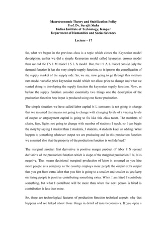
Keynesian supply function, first you will have the production function the next equation
is the labor demand function and then you have the last two equation one is an equation
and the other one I assume W is equal to W naught. Now, if there is surplus level also
they are exists surplus labor, so there is excess supply in the labor market.
So, the labor market diagram if you draw what I had is the following the wage rate is
here, so if there is surplus labor what will the labor supply function determine at W
naught the among that is supply from the point of view of surplus labor. There is an
excess supply if there is surplus labor excess supply is there then the short side of the
market determines what happen. So, the labor supply function is not very useful except
telling you that how much labor is available which is unemployed may be part of it
which are not using that is all it gives you the value it gives you the value of labor
supply.

5. Labor the supply function at W naught g N tells you the number gives you the amount of
labor supplied or available all right. So, it is not a very useful equation from the point of
view hour working with the model it is not very useful. Second point this W is equal to
W naught is equation can be removed by putting a W naught value here and W naught
value there will be substituting it. So, what we have after substitution and assumption
what we now have we have the production function and we have the labor demand
function is equal to W naught.
Nothing else remains as important for us, nothing else remain as important is anything
more important to us, nothing this equation and this equation other two important. Once
this one gives you with the number of people available and if you are not hiring, so it
tells you the number unemployed if we minus or subtract the people employed what is
the important. How many people employed will be given by the labor demand function
at W naught which is this one this is the number of people employed and this one is
simply the number of people supplied you can call that N S that W is equal to W naught.
So, the supply side of the keynesian supply function sorry the equation of the keynesian
supply function now reduces totally two equations the rest are not important anymore.
Once you know them what they are therefore from this two equations we should be able
to obtain the aggregate supply function. So, since they are we have not specify the
functional of form a linear function or nor linear function we cannot get the aggregate
supply function which can also be linear or nor linear function one. All we can do is I
can differentiate this and get the slope of the supply function which we did with the I S
function, L M function without specifying a functional form I S function L M function.
Then aggregate demand function I told you what the slope is going to be so just check
the slope of function.

6. (Refer Slide Time: 17:00)
So, slope of the aggregate supply function totally differentiate his d Y is equal to F N d N
and the second equation will have F N d P plus P F N again differentiated. So, F N, N is
equal to 0 because d W naught is 0 d W naught is 0, so it will be equal to 0 now from
here you can get the I am sorry F N, N nobody said anything d N is 0 F N, N d N is equal
to 0. Now, from the first equation you can get the expression for d N answers you did
there, so what you have is from this equation d N is equal to d Y over F N substitute
there substitute it in this equation.
So, what you have is F N d P plus P F N, N d N will be equal to d Y over F N is equal to
0 another than slope will be d P d Y. So, d P d Y slope of the function aggregate supply
function is equal to minus P F N, N divided by F N square d P d Y is equal to minus P F
N, N divided by F N square. Now, you know F N, N is negative F N square is the
positive term P is a positive term with the minus sign this is greater than 0.
So, this is the positive slope of the aggregate supply function this is the positive slope
that I talking about that I diagrammatically obtained in the previous class is the slope of
the aggregate supply function [FL]. Now, look at the fun here initially in the keynesian
cross model and in the I S L A model it assume very passive supply function which is
horizontal prices were fixed you remember that keynesian supply function was
horizontal prices were fixed. We said there by making that kind of assumption we can

7. make the model demand independent the supply is no longer playing an active role it is
just laying there.
So, depending upon where the demand curve is output will be determined the model was
entirely demand it with dependent or demand determined model aggregate supply was
horizontally price was fixed because horizontal line on the Y axis intersect is fix and that
was the price. Can you look at this supply function when that kind of situation is also
possible without telling you the story of excess supply existing in the market or excess
capacity existing in the market? So, company have excess capacity like big class room
what hardly in students there big building hardly any faculty their big campus hostels.
But, hardly any students living there so if you demand more education from I I T Kanpur
come there is no problem there is excess capacity that kind of a situation I talked about
can you look at this slope of the supply function. Technically speaking one assumptions
can make and give you a horizontal aggregate supply function one particular assumption
can give you horizontal aggregate supply function which is possible technically speaking
without getting into this words. A wage excess capacity on that come back to the
production function why would F and K naught the first derivative is F N [FL] and the
production function I drew was a aliened like this F N, N declining [FL].
Look at this function F N, N does not decline if F N, N is constant what happen is F N, N
0 a constant differentiate will give you 0 value. So, you can have a production function
which is linear where F N the slope of the production function is F N is constant slope of
liner line is a linear function is constants a straight line is constants you see that. So, what
you are saying is every time the company has somebody gets the same output F N is
constant margin product is constant what is marginal product when you hire a extra
person what is its contribution. There is the product in terms of output is constant I had
one person what extra output I get when I have the 100 extra person I get exactly same
amount contributed to my companies output.
So, a technical assumption like a linear production function F N is constant and the
production function is not curve like this is a straight line. Straight line will give you F N
constant can render d P d Y 0 which is the kind of a think we assumed initially, but I can
tell you now then you have no idea and I cannot be talking about the detail of the supply
function.

8. Only I say please assume the supply function to be perfectly elastic what is called an
economics it is a horizontal line with 0 slope, but you can see what kind of an
assumption will give you that [FL]. So, you can appreciate this point because you have
matured, now over the weeks you know more macroeconomics you know what the
stories are the algebraic behind this kind of story, now you can appreciate that, now let
us go something else.
(Refer Slide Time: 24:22)
The complete Keynesian model the demand side if you recall the demand side has I S L
M equation I S equation which is Y is equal to a naught plus C into one minus t Y plus I
r the L M equation you have M naught. Now, write naught P naught we are not in a fix
price model anymore price will be a variable I get supply function is upward sloping. So,
M naught not over P naught P naught any more is equal to h Y plus l r this you already
know then on the supply side which I just there are two more equations one is the
production function. The production function is Y is equal to F N K naught and the other
one was the labor demand function labor demand function.
What will be the labor demand function it will be P F N is equal to W naught I said two
equations are sufficient to consider the other one. Then go to substitution and the labor
supply function is re done assumption that tells only people available for work, but with
of surplus they not hire, so there are some unemployed people in the country. So, in
essentially of 4 equations call them if you want 1, 2, 3, 4 equations the 4 equation in a

9. model will be determine model if you have 4 unknown, 4 variables are solve. What are
the 4 dependent variable are indigenous variable that will be solved by the model the 4
variables are Y and r from the I S L M you know that Y and r are measured.
But, what are the other variables, now with the supply side yes you said the right thing
what is your name you yes, you have said the right thing I can, I can read your lips P
right is one of the variable and what is the other one you are murmuring. But, you do not
have the confidence to say it loudly because you do not have the confidence you
absolutely right P is one of the variable. Now, price will be determine and very good and
I just saw her lips she is looking at the board and murmuring, but not saying it loudly.
So, I encourage her to pushed her to say that yes absolutely right P is now a variable is
no longer fix price model, now you a have complete demands supply model were prices
are variable.
So, you can see how prices change in the economy is mature model is a complete model
Y r, P, N and, now if you do not mind what I would do I would from the first two
equation I would reduce the 4 equation model into 2 equation model. From the first two
equation I would eliminate r, suppose I ask you the question tell me what is the main
physical multiply in this model suppose I ask you the question which I am been asking
you right throughout.
(Refer Slide Time: 28:30)

10. What is d Y d G in this model how what how would you solve the best thing is
differentiate is two eliminate the r and differentiate this two can eliminate the N then r
and N gone we now have Y and N to be determined. So, let us do it, so what you would
have from 1 and 2 you get d Y is equal to d G, d G plus C into 1 minus t d Y plus I r d r
the second equation will be let us assume money supply constant with the timing we
consider the multi policy later d Y d N. So, it will be m naught over P square minus d P
am I correct if you differentiate P minus M naught over P square d P is equal to h d Y
plus l r d r.
Now, you can see you can get a d r value here, so the d r value would be minus bracket
M naught over P square d P minus h d Y divided by l r put that number in this d r. So,
what you have is d Y is equal to d G plus C into 1 minus t d Y then minus this bracket
term which is M naught over P square d P and minus h d Y bracket close you will have I
r over l r [FL] plus.
So, this kind of a thing you will get call this I can rearrange the terms, here I will get if I
club the d Y terms then I will have 1 minus C into 1 minus t. Then minus it will be plus h
I r divided by l r d Y and that minus P into that can comes on the left hand side is an
indigenous variable price we bringing all the indigenous variable to the left. So, it will be
plus M naught I r divided by P square l r d P is equal to only things that remains is d G
only thing that remains is d G call this equation number 5, call this equation number 5.
Now, from 3 and 4 we have d Y is equal to F N d N and F N d P then plus P F N, N d P d
N is equal to 0 from this equation we have d N is equal to d Y over F N substitute.
Then you have F N d P plus P F N, N over F N into d Y is equal to 0 all this equation 6
find out if this 2 algebra is or not call equation that one 6 and 2 equation all this 5 and 6 I
eliminate the r substitution, I eliminate the d N substitution. So, I have 2 equations and
two unknowns are there P and d Y the P N d Y, now copy down they I would tell you
from now onwards I would be using matrix algebraic to solve because next few topics at
least one topic would required a lot of matrix algebraic famous rule to solve.
Thus, to get the multiples instead through substitution famous rule use famous rule
matrixes said them up is very nice and easy to solve them. So, if you copied it, now once
you copied the equations down what I would do and this is the method I will keep till the
last topic life is much simpler to gets this equation solved this multipliers not equation to

11. get the multipliers. To obtain the multipliers we can just use this equations 5 and 6, so
what I have from 5 and 6 if I club and make 2 columns one for the d Y column one for
the d P column.
(Refer Slide Time: 35:21)
Then from the first equation that d Y column as 1 minus C into 1 minus t plus I r h over l
r this is the d Y column the second column will be the d P what is the d P term M naught,
M naught I r over P l r. From the first equation 5, I have P square there P square from the
second equation d Y column has P F N, N over F N I think P F N, N over F N and d P
column has F N. So, this is my matrix which multiplied by column vector d Y d P this is
how you can use matrix to write the equations.
So, what you are saying this first row is multiply with this column the first elements is
first element, here plus the second element is second element second. For the second
equation again this row is multiplied with this column vector, so first element d Y plus
this with the second element, here that is what you do and is a multiplier which is one
loom variable. Here, that is in first equation hexogen variable on the right all hexogen
variables written in the right hand side. So, hexogen variable is d G so if I have a d G
column, here d G has one value in the first equation second equation there is no d G
variables.
So, it will take a 0 value, so the column vector here would be one 0 for d G, so this is the
method I will be using now till the last topic it is easier to solve. In fact, we could have

12. the 4 equation right way in the matrix, but to work with 4 columns sorry 2 columns, but
4 rows is much more compressive. So, I eliminated simplify the system 2 equation, now
the two equation 2 by 2 equation is much better 2 by 2 matrix is much better all right,
now what I have here is that you know that d G will solved. While d Y d G will be the
determinate of the matrix with d Y d G d Y column will be replace by one and 0, so it
will be I am using the straight line for determinate one 0.
The second element will remain d Y column will be replace by the d G column, vector
the second column would be remain which is M naught I r divided by P square and the
second one is F N. That is the determinate of as the determinate of in the top and divided
by determinate of the entire matrix which is 1 minus C into 1 minus t plus I r h over l r
and you have M naught of the determinate of the entire matrix. Now, you can find out
the determinate right away you know how to get it one multiply this diagonals terms are
multiply minus half diagonals term product that is the determinate the product of the
diagonals term minus half diagonals term.
So, it will be F N minus 0 into that 0 wonderful nothing to be done there divided by
complication F N into this F N into 1 minus C into 1 minus C plus I r 8 over l r minus P,
F N, F N into that P my goodness. It is mess minus P, F N, N divided by F N into M
naught I r M naught I r over P square l r two terms, so this is your d Y d G. Now, we
need a better life less simplify and make it comparable with the other multiplies that we
have seen the d Y d G in the previous case d Y d G.
In the previous case you can see one thing you can divide numerator determine by F N
cancels out one will be there which is great news. Earlier divide d G is to have 1 in the
numerators, so let 1 be there and, here when you divided by F N it becomes F N square,
it becomes F N square, so what you have.

13. (Refer Slide Time: 41:43)
Therefore, d Y d G is equal to 1 divided by wonderful 1 minus C into 1 minus t plus I r h
over l r and, here minus P F N, N over F N square into M naught I r divided by P square l
r. Now, you can see one thing here P F N, N over F N square what was that you just add
this expression to day morning the slope of the aggregate supply function slope of the
aggregate supply function which is visible there. This is, this is the old multipliers 1 over
1 minus C into I S L M multiply 1 over 1 minus C into 1 minus t plus I r h by l r I S L M
multiply.
Now, minus at bunch of terms is it a positive term or negative term this is positive I r l r
both are negative this ratio is positive here is a negative. But, with the minus, so entire
thing is a positive, so what do you saying are quite disturbing, now with the keynesian
cross model to I S L M the multiplied we can with. Now, complete keynesian called
multiply as weekend because you add a positive term to denominated, so the ratio value
falls.
So, the multiply is becoming is more and more weak the expenditure multiplier the more
you make the more realistic with price changing etcetera we have to find out why it is
become weak we will find that diagrammatical it. But, just by looking at the algebra if
you want to compare this is very clear that you compare them the expenditure multiply
as become even weak with the supply function. In the keynesian model it is something is

14. happening because we checked that he price move basically why is price move making
things weaker we have to find out.
Now, this is the slope of the demand function M naught I r over P square l r what was the
slope of aggregate demand function in the previous class I had I just want to check that r
what was the slope of aggregate demand function from I s and L M. You get the
aggregate demand function 1 minus C into 1 minus t divided by divided by I minus I r
this term divided by this term this term divided by inwards of this inwards of this no this
is this [FL] is very funny. So, the demand function slope is not directly there parts of
their separated from each other line there, but not together, but the supply function slope
is interact this is the aggregate supply function slope that is interact there.
This whole thing is a positive number, this whole thing this entire thing with the minus
sign is greater than 0. So, the physical policy multiplier expenditure has become weaker
the strength has gone down, so we need to find out why is the strength gone down I
notice one thing I just said that you get the horizontal aggregate supply function. If F N,
N is 0 F double N is 0, I was telling you the technical assumption give you that if F N, N
is 0 this whole term is 0 your back to the old multiply I S L M. You see that you back to
the old multiply I S L M one over the first term second term [FL] whichever I am trying
to tell you few minutes back.
So, we get that result this consistent what I am doing what I told you the student is
consistent, now we reaching 50, 55 minutes back, so the after end of the one class. So,
what I plan to do before I give you intention why the multiply become week need I
diagram, so why is the multiplier getting weaker is weak come to the previous multiply
the previous module I need diagram to talk about. I would consider only two diagrams, I
would not complicate if I would take the I S L M diagram and I will take the aggregate
supply aggregate demand diagram 2 parts.

15. (Refer Slide Time: 47:54)
So, first is the I S L M diagram and underneath I have the aggregate demand, I aggregate
supply diagram suppose demand function is like this aggregate demand. Suppose the
supply function like this aggregate supply and this equilibrium point corresponds to also
equilibrium in the demand side. So, this is I S and suppose this is L M and this is a rate
of interest, some L M has the money supply and price initially say P naught that means
this is the price P naught and this is the output level in the economic which is demanded
and supply Y naught.
So, you get the integration of aggregate supply function because on the demand curve it
is all this means your intersection of I S L M because I S L M together gives you demand
curve. So, every point on the demand curve it equilibrium point in the diagram you will
be require both the equations to get the demand function and suppose this is the supply
function. If you go the labor market, there is labor demand function and the production
function and I am not joining them I am just drawing these two diagrams.
Now, this is the story, suppose there is the government expenditure increase according to
the I S L M model according to the I S L M model the I S curve will shift equilibrium
point will come of I S L M intersection remember that. That means new point should
correspond to a demand function the question is where the demand function is, so the
demand function must be shifting because prices are constant. So, if I shift because of

16. government expenditure increase then this point and since prices have not change are the
new point on the demand curve that is no demand curve.
So, essentially what we say is that prices are not change look L M is the same L M prices
if prices change L M will shift. So, prices are not changing, so the new point on the I S L
M correspond to new point on a demand curve which does not exist that means the new
demand curve some of their. If you remember the aggregate demand slope if G increases
as aggregate demand shift parallel L, so you have a parlor shift in the demand function
call that A D 1 parallel shift in the demand function called A D 1 this is say A D naught
A D 1 and A D naught.
So, that is the demand function, so when A D 1 is increases what is happening the story
is that the firm running down inventory to meets the extra demand in the aggregate
demand this line by the way has been much of a parallel line. It is the parallel line this
original equilibrium point and this new point which corresponding to the I S L M
intersection this new point which corresponds to I S L M intersection is creating a day
excess demand for goods. The potential demand is creating excess demand for goods
which is equal to this gap because the supply line is here, so the actual supply in
economic is here.
But, the potential demand gone up to point this is what I am trying to say, now with I S L
M intersection when you reach suppose the economy as met that, so inventory
adjustment actual output has been increase. So, the potential demand has gone their
which will rest on equilibrium here, but the supply is still here does not excess demand
you can call these points. You can this say this one is called may be E 1 and this one can
be called E 2, so E 1, E 2 minus E 1 is equal to excess demand for goods E 2 minus E 1
equal to excess demand for goods. When in a market which we teach in a
macroeconomic their excess demand there is output threshold on prices because of the
potential demand.
Now, prices start increasing and according to macroeconomic theory we know as prices
increase, companies have incentive to supply more. So, the question is how do prices
increase one theory says as prices increase all right the L M curve will start shifting
backwards because L M is M over fixed over P as P increases the left hand value of M
over P falls. So, the right hand side can falls also and what happens is that adjustment

17. comes to rate interest increase speculated demand falling etcetera. So, as its increases
prices increases you can say along the demand curve the prices start moving upwards
along the demand curve the prices start moving upwards and L M curve start shifting
backwards point is where will reach the equilibrium.
The new equilibrium is reached at the intersection of the supply and the new demand, so
the L M curve will shift backwards till it reaches equilibrium in the I S L M diagram
somewhere in the new I S and a new L M. That will a merge which also will be a parlor
shift in the L M curve call that may be some L M 1, it finally goes to where prices in the
economy would have reason to P one and output will also increase. But, it will only
increase up to Y 1 and this is the new point of equilibrium where you have M naught
value of money supply divided by P 1 value of prices.
So, adjustment goes up along the demand curve economic start adjusting the final level
of output that the economy produces Y 1, so in the normalize view would have come to
the green point. But, price increase on a backward shift left was shift in the L M reduces
output further reduces demand further. So, the multiply is essentially becoming very
weak that is what the multiply will weak this output level this green line this green line is
the I S L M result. But, we come to the pink line which is the complete keynesian model
price flexibility, so price increase reduces demand in the economy reduces output in the
economic also it falls why would company produces more company would produce less.
So, you see why the multiplier is weaker because from the Y to pink that distance that
distance is less than from white to green white to green was distance in the I S L M
which was one over 1 minus 1 over t plus I r over h l r. Now, the last component addition
in the denominator of the multiplier is essentially saying that the multiplier weak which
is you go up to the pink point Y 1 to Y the multiply become weaker. You can see excess
demand increases prices and reduces demand, so that is why people say inflation is bad
for the country because what inflation does is doing purchases power people buy less
company also produce less.
Here, it is gradual upward shift in prices and you stops inflation upward is the dynamic
variable because prices continuously rise that is why people say inflation is bad because
what inflation does is not purchases power. You demand less excuse me [FL] your
purchasing power loads and you buy less and the company also produce less economy

18. produces less. Now, do we see this multiply expenditure multiply why it has become
weak you see that, thus, yes.
Student: E 1 is the white one or pink one.
[FL] what, yes.
Student: Among those points, E 1 is the white one or pink one.
P 1 is with the I S and the green A D 1.
Student: E 1.
(Refer Slide Time: 01:00:24)
No, E 1 is the white point, let me use white chalk E 1, let us use the green chalk here E 2
and let us use the pink chalk there this one E 3, now is it clear becoming the perfection
diagram I will start painting after course ends [FL]. So, price increase is the culprit and
you can also say sir tell us more why prices increases in culprits well when prices
increase. Then for money market equilibrium since the left hand side L M equation value
falls the right hand side should also falls the match and the right hand side rate of interest
increase.
Now, rate of interest increases private investment cannot increase through the potential,
so there is a crowding out through the back door coming one. Crowding out is their rate
of interest increase, I S shifts out of the crowding are coming with L M backward

19. shifting and increasing rate of interest is in further which is an indirect crowding rate
coming into the picture. Look at the I S L M diagram, first crowding out from this point
to that point, from this point to the green point we learnt this crowding out. This is the
rate of interest which is say r naught and this would have been the rate of interest which
is something say r prime naught.
Now, with L M shifting there is even higher interest rate which woes up further, so rate
of interest increases in further to r 1, so there is a double crowding out first crowding out
is from r naught to r 1. Then next crowding out is coming indirect effect by prices
increase money market adjustment that you go to r prime not r 1. So, the full potential of
the exponentially physical policy cannot be realized because the two rounds at least
crowding out one direct I shifted which we learnt in the I S L M model. Now, the second
round coming from the prices increasing and money market adjustment which we call
further increase in real rate of interest, so the multiply it is like unsigned to run my full
potential.
First I get a hardly on the soled something stop me some sloes not even then there is the
strong wing from the opposite direction which slows me further down. So, I run slowly, I
do go the distance, but that is not my full potential without those uneven surfaces and the
strong wing coming from the opposite direction I can run must faster, I reach up longer
distance. But, I cannot 2 rounds of crowding going out you see that, now the algebraic
part of monetary policy multiply you can work it out yourself d Y d M you can do that.
But, what happen in diagrammatically this very similar situation in case of money supply
multiplier, let us check that out d Y d M, d Y d M.

20. (Refer Slide Time: 01:04:47)
You can find out the multiplies uses, so using algebra, but diagrammatically what is
happening I would draw the I S L M diagram in this is the initial points equilibrium
points. Now, let us talk out money supply multiply what happens what was the color I
was using the green color the money multiplier will now monetary policy expentially
will shift L M out. So, you will get L M curve like this a parallel shift parallel shift in the
L M, so you have M 1, but prices are the same M 1 increased, M 1 is greater than M
naught.
So, the aggregate demand curve will shift at the same price it will be same kind of logic
it will be somewhere here because the demand curve will always have intersection of I S
L M will those two equations are used to get the demand curve. So, the aggregate
demand curve will shift not parallel probably anyway you can find out A D 1, now
excess demand is created again output is at Y naught demand as gone there prices will
start increasing.
When prices starts increasing along the demand curve prices are increasing along the
demand curve L M will start shifting backwards M 1 is there increase value. But, P 1 is
now increases P, so ratio falls it is just shifting backwards and it will reach a new
equilibrium which is some L M 2 which will have some M 1 some divided by some new
price P 1 this is L M two it will shift backwards. So, first the green line shifted L M, here

21. then it is going backwards is moving backwards the L M curve is moving backwards
curves and where you have a higher level of price.
Now, P 1 and of course some higher level of output Y 1 and you do not have the full
potential of the output up to green line. You do not have the green line potential the
green line potential would have been possible if you are a fix aggregate model supply
function horizontal, but since prices are increasing L M will go out and come back a little
bit. So, if you work the algebra of d Y d M the way I got d Y d G you will see that
multiply is weaker compare to the d Y d M multiplier under this multiplier is weaker. It
clearly says that because prices will increase as prices increase you can see the gap
between demand and supply strings [FL].
The gap is this much initially as much is increases it eliminates excess demand and
supply also increasing along supply line and then they meet here at the pink point where
the 0 excess demands, it will be, has been reach. You will see d Y d N multiply in this
case is less than the d Y d M multiply we obtained algebraically also in the I S L M
model that value is less you can check the doubt yourself this a little bit of work. You
can do what is the d Y d M algebra using matrix algebraic you do that, you have to
differentiate d M also which will d M component.
Which will be multiplied by 1 over P which you keep on the right hand side and also d B
differentiate will be there and you can get the d Y d N. So, the money supply multiplier
also become weaker, so just now physical policy is, now weaker monetary policy is also
become weak compare to the I S L M the prices or fixed. So, none of the policies are
really working none of the policies are working if prices are increasing if prices fixed
then you solve right when prices are increasing none of them really working. So, better
situation would be if prices increasing continuously you have a supply curve based
policy if the supply can shift you can change the prices increase output also if supply can
shift as suppose to demand shifting.
If supply curve shift is counters inflation put down load prices as well as output will
increase demand management policy become weaker if the price is increasing. So, in
India today at the past year, so we are having strong inflations and government of India
and monetary or not R B I what they have been find is reducing money supply and
control inflation reducing money supply means shifting L M naught. But, shifting L M

22. backwards, so that aggregate demand shifts backward and trying to control prices then I
have not been able to do much that.
But, that has a dangerous output value which is happening a better policy would have
been through a supply management if supply curve can be shifted out instead of
monetary management by constructions monetary policy which is L M shifting
backward. The dangerous prices will have tendency to come down inflation has come
down, but the cost of output and in India there is growth rate following industrial output
all that happening this model explains that gives the feeling that this is what you would
expect. If R B I government has contract monetary policy as a tool to control inflation,
but we do not have inflation, here we have static model prices goes up in steps and stops.
But, in the dynamic model, but this gives you the free that continuously what will
happen, so the policy are still there pursuing it very adamant incorrect policies
completely incorrect policies right from the beginning. In the recession they not brought
a senior decision in to the economy which would not come, not so much some damping
would have been from the external sector not so much. To be honest with you keynesian
model is really over, but I can I want ask you a few things few questions before I close it
look at the complete look at the labor market diagram wage rate.
Look at the diagram you had wage rate fix labor demand labor supply and aggregate
supply function I agreed the supply function previous days class aggregate supply
function will diagrammatically drew that you have the diagram with you. Now, you tell
me if there is an upward division in wages what will happen upward division in wages
what will happen I am quisling you a little bit. There is an upward division in wages look
at the diagram W lines goes up from W naught to and above a higher line say W 1 line
above W naught, what will happen. What is the effect that you will have immediately in
economy, what the thing you will have in economy output will fall, aggregate supply
function will shift to the left you see that aggregate supply function will shift to the left
in this model.
You can obtain a d Y d W if you want which I put d W is equal to 0 in the supply
function you can have d W non zero and then solve d Y d W no problem. You will get a
result there negative result inverse result it should be negative W goes up output falls
[FL], another question I am asking you. Suppose there is the technological improvement

23. massive technological improvement came through then margin product line shift to the
line W remains the same and aggregate supply will shift to the right. Now, in I S L M in
aggregate demand if aggregate supply shift to the right what will happen in prices
economy what will happen go up and down, down the money wages are fixed.
So, what happens in real wage real wages increase you see, now you can use your mind
in the model to talk about many important things with speak on T V sometime it does not
make any sense. But, now it will make some sense to you the real wages in the economy
go up which every economy wants real wage means real income, so I can buy more
goods no juts tell me 1000 rupees more. But, I want my real income go up so that I can
buy more goods more dominate tips which my children would love that is what they
want real expenditure to go up while they want many things which is not possible.
But, usually that what people loves everybody likes economic likes people likes real
income to go up, now you see this things you can connect them. So, to be honest with
you 15 minutes short, but I have really come to the end of the discussion of the
keynesian model my point is whether there is a topic I called that supply side model. It is
a very simple model supply side model whether I will discuss that or not I will decided
yet, so I will skip that I will go to the exchanges systems you will see in our topics
balance of payment account. Then the last model algebraic model to deal with open
economic issue I will do that in a next week, you do not mind if I close today, it is all
right.