Transiting Exoplanets

Transiting Exoplanets
Ian Beagles and Eli Todd 16APR2014
Department of Physics and Astronomy, Northern Arizona University, Flagstaff, Arizona 86001
Abstract
The Kepler-9 system holds great scientific value as the first multi-planetary system found using
the photometric transit method. The transit time variations (TTVs) for Kepler-9’s planets are the first to
have been found in another system. Using transit data and radial velocity data from Holman et al.
(2010), we found the radius, period, TTV, semi-major axis, mass, and density for Kepler-9b, Kepler-9c,
and where possible, Kepler-9d. We found that Kepler-9b and 9c are Saturn-sized planets with 19.24 and
39.08 day periods respectively and Kepler-9d is a super-Earth-sized planet with a period of 1.59 days.
1. Introduction
The Kepler mission is designed to survey a section of the Milky Way Galaxy to discover the
frequency of Earth-size planets orbiting in the habitable zone of stars. Kepler is able to detect exoplanets
by observing the dimming of a star’s light when a planet passes in front of its host star. Several traits of
the planet can be calculated from the characteristics of the dip in the star’s light. The planet’s orbital
period can be determined by the frequency of the planet’s transits and the planet’s size is ascertained
by the transit depth. Other system and planetary properties are suggested by or refined from using data
from transit information. Multiple planets in the system are suggested by variations in a planet’s transit
duration. Because of the nature of detecting planetary transits, the planet’s inclination is limited to the
size of its star. This limit on inclination allows the mass and density of the planet to be calculated to a
high degree of accuracy when combined with radial velocity data.
Doppler spectroscopy, also known as the radial velocity method, uses the Doppler shifts in the
spectrum of a star to detect exoplanets. Using the radial velocity method, a minimum mass for the
planet orbiting the star can be determined from the spectral shifts caused by the planet. The actual
mass for the planet cannot be calculated from the radial velocity method without knowing the planet’s
inclination with respect to us. The planet’s inclination can be found if spectral lines for the planet can be
separated from the star’s spectral lines. Finding the inclination for the planets in a system where the
planets transit is much easier since the inclination is limited by the size of the star.
To date, Kepler has found over 900 confirmed exoplanets with ~4,000 other planetary
candidates (NASA 2013). The Kepler-9 system was first detected by Kepler in 2010 and was the first
multi-planetary system to be discovered using the transit method. Two gas giants and a super-Earth
have all been detected orbiting Kepler-9. The Kepler-9 system is of great interest as it is the first
extrasolar system whose planetary transit time variations (TTVs) have been obtained.
2. Data
The data provided to us contained data from the Kepler mission’s observations of the Kepler-9
system. This data was refined by Holman et al. in their 2010 article (hereafter H2010) to indicate which
data points correlated to the noise of Kepler-9 and which to the transits of Kepler-9’s planets. We then
used the flags provided by Holman et al. to color code the data provided by H2010 in order to easily
identify the transits of Kepler-9’s planets (Fig. 1). As of 2010 the existence of Kepler-9d was only posited

via TTVs in Kepler-9b and 9d by Holman & Murray in their 2005 article (hereafter H2005), and as can be
seen in Fig. 1 the transits of Kepler-9d lie almost entirely within the noise of Kepler-9. The existence of
Kepler-9d was later confirmed by Torres et al. in 2011 (hereafter T2011) via extensive computer
modeling and data analysis.
Using the data provided by H2010, we were able to determine: the periods of Kepler-9’s
planets, the TTVs for Kepler-9b and 9c, the semi-major axes of the planets, their radii, and using
photometric data, the mass and density of 9c and, the mass and density of both 9b and 9c using radial
velocity data provided in Holman et al. Supplementary Online Material 2010 (hereafter SOM).
Orbital Periods:
Using the transit flags from the data of H2010 we used MatLab separate out the transits of
Kepler-9b (Fig. 2), 9c (Fig. 4) and 9d (Fig. 6) and to then determine the mean periods of each planet
(Table 1), along with the standard deviation in those values. For 9b and 9c we used the lowest value of
the flagged data in each transit as the midpoint of each transit. For 9d we used the flagged data in the
range of BJD 78.5098-94.3872. This period lies in the first quarter of observation and within the first and
50 100 150 200 250 300
0.993
0.994
0.995
0.996
0.997
0.998
0.999
1
1.001
1.002
1.003
Days from BJD 2454900 (Days)
DetrendedKepler-9Flux(W/m2
)
Detrended Light Curve of Kepler-9 Data
Detrended Flux
Planet B
Planet C
Planet D
Planets B&D
Planets C&D
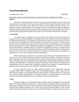
Figure 1: The detrended light curve data of the Kepler-9 system, color coded by the noise of Kepler-9 and the transits of its
planets. It can be seen that the transits of 9d (the red dots) lie almost entirely in the noise of Kepler-9. The discontinuities in
the data correspond to the breaks in the quarters, when Kepler-9 moves to a different detector after the rotation of the
Kepler spacecraft.

second orbits of 9b. We chose this range in order to minimize potential perturbations by 9b and error
from renormalization of data after the quarterly change to a different detector on the Kepler spacecraft
(H2010).
Kepler-9 Planetary Periods Period (Days) Error (days)
Planet 9b 19.2414 ±0.0263
Planet 9c 39.0816 ±0.0913
Planet 9d 1.5877 ±0.0610
Table 1: The mean orbital periods (in days) of the Kepler-9 planets as calculated using the H2010 data and MatLab. These
results lie within error tolerances of the values published in H2010.
While we chose the lowest valued points of the data flagged as transits for 9d within our range, as can
be seen (Fig. 7), these flagged transits do not possess the same symmetry as the flagged transits of
planets 9b (Fig. 3) and 9c (Fig. 5). The values that we calculated for these periods and their attendant
error have them straddle the values and error that were published in H2010 and for 9d, T2011.
Figure 2: The detrended light curve data of Kepler-9, filtered for the transits of planet 9b (the blue and magenta dots) and the
noise of Kepler-9 (the black dots). As can be seen, the third and seventh transits of 9b are missing. This is due to the quarterly
rotation of the Kepler spacecraft.

134.75 134.8 134.85 134.9 134.95 135 135.05 135.1 135.15 135.2
0.993
0.994
0.995
0.996
0.997
0.998
0.999
1
1.001
)
Detrended Light Curve of Kepler-9b Data
Detrended Flux
Planet B
Planet B&D
Figure 3: A magnified image of the fourth transit of Kepler-9b, with the vertical scale held constant. This view shows the
expected symmetrical nature of the dip in luminosity as 9b transits Kepler-9.
50 100 150 200 250 300
0.993
0.994
0.995
0.996
0.997
0.998
0.999
1
1.001
)
Detrended Light Curve of Kepler-9c Data
Detrended Flux
Planet C
Planet C&D
Figure 4: The detrended light curve data of Kepler-9, filtered for the transits of planet 9c (the green dots) and the noise
of Kepler-9 (the black dots). Here, all of the transits of 9c can be seen, as they did not coincide with the quarterly
rotation of the Kepler spacecraft.

263.8 263.9 264 264.1 264.2 264.3 264.4 264.5 264.6 264.7
0.993
0.994
0.995
0.996
0.997
0.998
0.999
1
1.001
) Detrended Light Curve of Kepler-9c Data
Detrended Flux
Planet C
Planet C&D
Figure 5: A magnified image of the sixth transit of Kepler-9c, with the vertical scale held constant. This view shows the expected
symmetry in the nature of the dip in luminosity as 9c transits Kepler-9.
50 100 150 200 250 300
0.997
0.998
0.999
1
1.001
1.002
1.003
)
Detrended Light Curve of Kepler-9d Data
Detrended Flux
Planet D
Figure 6: The detrended light curve data of Kepler-9, filtered for the transits of planet 9d (the red dots) and the noise of
Kepler-9 (the black dots). Here, it can be seen that the data flagged as transits of 9d lie almost completely within the noise of
Kepler-9.

Planetary Radii:
Using the periods that we had calculated and equation 1, we then calculated the radii of planets
9b, 9c and 9d (Table 2) using our code in MatLab.
𝑅 𝑝 = 𝑅∗√∆𝐹𝑙𝑢𝑥 (1).
Here; Rp is the radius of the plant in question, R∗ is the radius of Kepler-9, which was given to be 1.1Rʘ
and ΔFlux is the mean value of the flux when there is no transit i.e. 1 minus the flux at the mid-point of
the transit all divided by the mean value of the flux when there is no transit, again, 1 (Seager and
Mallen-Ornelas 2003).
The values that we calculated, along with the standard deviation in those calculations put them
on either side of the range of values published in H2010 and in the case of 9d, T2011.
75 76 77 78 79 80 81 82
0.997
0.998
0.999
1
1.001
1.002
1.003
)
Detrended Light Curve of Kepler-9d Data
Detrended Flux
Planet D
Figure 7: A magnified image of the transits of Kepler-9d from BJD 75 - 82, with the vertical scale held constant. This plot
displays that the data flagged as 9d transits do not exhibit the characteristic symmetry in the luminosity dip that is found in
the transit data for planets 9b and 9c.

Kepler-9
Planetary Radii
Radius in Solar
Radii (Rp/Rʘ)
Error in Radius
(Rʘ)
Radius in
Jupiter Radii
(Rp/RJ)
Error in Radius
(RJ)
Planet 9b 0.0904 0.0011 0.8794 0.0103
Planet 9c 0.0875 0.0013 0.8515 0.0122
Planet 9d 0.0253 0.0046 0.2466 0.0444
Table 2: The mean Radii of Planets 9b, 9c and 9d in both solar radii and Jupiter Radii, along with the standard deviation in
those calculations. These values are within the error tolerance of the values published in H2010.
TTV:
Having calculated the average period of each planet in Kepler-9, we then plotted the predicted
mid-point of the transits (in BJD) along with the observed mid-points of the transits (in BJD) of 9b and 9c
(Figs. 8 and 11 respectively). We then used MatLab to find the best fit for the TTVs of 9b and 9c (Table
3). The error in the TTV calculations is large, but the values that we calculated for TTV of 9b and 9c still
encompass the values published in H2010.
Transit Time Variances TTV (Days) Error (Days)
Planet 9b -0.0127 ±0.0196
Planet 9c +0.0444 ±0.101
Table 3: The TTV values that we derived using the Kepler-9 data. Though the standard deviation in the TTVs is large, our
values are still consistent with those published in H2010.
Figure 8: A plot of the predicted and observed midpoints of the transits for Kepler-9b. The actual transits (black dots) are off-
set from the predicted Transits (red dots) for clarity.
50 100 150 200 250 300
0.9
1
1.1
1.2
1.3
1.4
1.5
Off-SetofY-AxisforVisibilityofDataPoints
Actual Transits vs. Predicted Transits for Kepler-9b
Actual Transits (black)
Predicted Transits (red)

Figure 9: A zoomed-in view of the last transit of 9c. This view of the predicted and actual midpoints of the transits, better
display the TTV as a function of time.
Figure 10: A plot of the predicted and observed midpoints of the transits for Kepler-9c. The actual transits (black dots) are
off-set from the predicted Transits (red dots) for clarity.
153.8 153.9 154 154.1 154.2 154.3 154.4 154.5 154.6
0.9
1
1.1
1.2
1.3
1.4
1.5
Actual Transits vs. Predicted Transits for Kepler-9b
50 100 150 200 250 300
0.9
1
1.1
1.2
1.3
1.4
1.5
Actual Transits vs. Predicted Transits for Kepler-9c

Figure 11: A zoomed-in view of the last transit of 9c. This view of the predicted and actual midpoints of the transits, better
display the TTV as a function of time.
Semi-major Axes:
Once we had calculated the values for planetary periods, radii, and TTV. We were then able to
calculate the semi-major-axes of the planets in the Kepler-9 system (Table 4) using the non-Newtonian
form of Kepler’s Third Law (Eqn. 2) and MatLab.
𝑎 𝑝 = √ 𝑃𝑝
2 ∗ 𝑀∗
3
(2).
Here; ap is the semi-major axis of the planet in question (in AU), Pp is the period of the planet in question
(in earth years) and M∗is the mass of the star that the planet in question orbits, in our case the mass of
Kepler-9 is taken to be one solar mass.
Kepler-9 Planetary Semi-
Major Axes
Semi-Major Axis: a
(AU)
Error
(AU)
Planet 9b 0.1405 ±0.0263
Planet 9c 0.2251 ±0.0913
Planet 9d 0.0266 ±0.0610
Table 4: The values that we calculated for the semi-major axes of Kepler-9b, 9c and 9d, along with their attendant error
tolerances. These values are within the error tolerances of the values published in H2010 and T2011.
The values that we obtained for the semi-major axes of planets Kepler-9b, 9c and 9d, when taking into
account their standard deviations, agreed with those values published in H2010 and T2011.
262.5 263 263.5 264 264.5 265 265.5 266
0.9
1
1.1
1.2
1.3
1.4
1.5
Actual Transits vs. Predicted Transits for Kepler-9c

Calculation of Mass from Photometric Data:
Using the previously derived data and equation 3 (H2005), we were then able to calculate the
mass of Kepler-9c (Table 5) using the eccentricities of 9b and 9c as found in SOM. We then calculated
the density of 9c as mass per unit volume (g/cm3
) (Table 5).
𝑀 𝑐
𝑀∗
=
𝑇𝑇𝑉 𝑏[1−√2(
𝑎 𝑏
𝑎 𝑐−(1−𝑒 𝑐)
)
3
2
]2
45𝜋∗𝑃 𝑏[
𝑎 𝑏
𝑎 𝑐−(1−𝑒 𝑐)
]3
(3).
Here; Mc is the mass of Kepler-9c, 𝑀∗ is the mass of Kepler-9 (taken to be 1 solar mass), TTVb is the
transit time variation for 9b, ab is the semi-major axis of 9b, ac is the semi-major axis of 9c, Pb is the
period of 9b, and ec is the eccentricity of 9c’c orbit. All of these values were converted into SI units.
Photometric
Calculation of
Kepler-9c’s Mass
and Density
Mass
(kg)
Mass in
Solar
Masses
(MC/ Mʘ)
Error in
Solar Mass
(Mʘ)
Density
(g/cm3)
Error in
Density
(g/cm3)
Planet 9c 7.4477*1024
0.0039 ±0.0951 0.0078814 0.0008738
Table 5: The mass of Kepler-9c as calculated using the photometric data of the Kepler spacecraft. This value is not close to
the values that were published in H2010, but that is to be expected, as the error in out TTVs was large and this method of
mass derivation is known to be inaccurate.
Our values for the mass of Kepler-9c, in solar masses, and its density were off by 2 orders of magnitude.
This can be accounted for by the compounding of all of the experimental uncertainties contained in all
of the previous calculations used to obtain the values used for these calculations. This is one of the
reasons why calculating mass from photometric data is known to be wildly inaccurate.
Calculation of Masses from Radial Velocity Data:
Lastly, we used radial velocity data provided in SOM to determine the half-amplitude of the
radial velocity curve: K (Table 6), and equation 4 to recalculate the mass and density for Kepler-9c as
well as the mass and density of Kepler-9b (Table 7).
𝑀 𝑝 = 𝑣𝑟,∗√
𝑀∗ 𝑎 𝑝
𝐺
(4).
Here; Mp is the mass of the planet in question, vr,* is the radial velocity of Kepler-9, M∗ is the mass of
Kepler-9 (taken to be one solar mass), ap is the semi-major axis of the planet in question, and G is the
universal constant.
Half-amplitude of Kepler-9
Radial Velocity Curve (K)
K of Kepler-9 Planet
(m/s)
Error
(m/s)
Planet 9b 21.4200 ±0.0849
Planet 9c 12.5200 ±0.1067
Table 6: The values of K (the half-amplitude of the radial velocity curve) calculated from data in SOM, along with their errors.

We needed to calculate K in order to get the radial velocity of Kepler-9. As K = v∗sin(i), where i is
the inclination of the orbital plane of the planet with respect to the line of sight of the observer, and as
we take the value of sin(i) to approach unity then we can approximate K = v∗, where v∗ is the orbital
velocity of Kepler-9. We can also approximate the orbital velocity of Kepler-9 as the radial velocity of
Kepler-9 at these distances, hencevr,∗ = v∗.
Mass and
Density of
Kepler-9
Planets
Mass of
Planet
(kg)
Mass in
Jupiter
Masses
(Mp/MJ)
Error in
Jupiter Mass
(MJ)
Density of
Planets
(g/cm3)
Error in
Density
(g/cm3)
Planet 9b 5.3618*1026
0.2824 0.0888 0.5150 ±.0011
Planet 9c 3.9668*1026
0.2089 0.1400 0.4197 ±.0013
Table 7: The recalculated values of the masses and densities of Kepler-9b and 9c. These values agree very closely with the
values published in H2010.
The values that we obtained via this method agree with the published values (H2010) to within the error
tolerances.
3. Discussion of Results
From our results we were able to see that the ratio of the period of Kepler-9c’s period to 9b’s
period was 2.0279. This indicates that 9c and 9b are in a 2:1 mean motion resonance (MMR), this finding
agrees also with the findings of H2010. Due to the fact that Kepler-9d was not confirmed until 2011 by
T2011, and that the data points for the transits of 9d reside in the noise of Kepler-9 in H2010’s data the
period of 9d has a large error relative to its magnitude. This error, though comparatively large, still
places our calculations in agreement with the values in H2010.
Our ranges for the values of the periods of the planets “bracket” H2010’s values. This holds true
for our values of semi-major axes, planetary radii, planetary masses, and densities as well, though this
only holds for the masses and densities derived through the radial velocity method. As can be seen,
(Table 5) the value for the mass and hence the value for the density of Kepler-9c, as derived via the
Photometric data are nowhere near the published values. These values are off by a factor of two orders
of magnitude. This only confirms that this method of mass calculation is an inaccurate one. These
inaccuracies arise from compounded experimental uncertainties contained within all of the previous
calculations used to derive each successive value.
Fortunately the radial velocity method of computing mass, and hence density, is a much more
accurate method. Our values for the masses and densities of 9b and 9c (Table 7) agree very closely with
those published in H2010.
From the values that we derived (Table 2) for the planetary radii, we were able to conclude that
both Kepler-9b and 9c were Saturn-sized planets while 9d is a super-Earth-sized planet. Also (Table 4)
that they all orbit very close to Kepler-9 relative to Earth’s orbit, much less Jupiter’s.
The error ranges are very high with respect to the magnitudes of the values (Table 3) of the TTVs
for 9b and 9c. While we used the same methods as we used to find the TTVs for both 9b and 9c on 9d,
the resulting numbers were not valid data. The error was significantly larger than the value of the
calculated TTV for 9d. This is mainly due to the transits of 9d being obscured by the noise of Kepler-9.

5. Conclusion
The values we calculated for the Kepler-9 system agreed with the published values in H2010 and
T2011. We were limited to using the provided data and equations instead of using H2010’s more
complex and sophisticated modeling techniques. Our method of calculating values for the Kepler-9
system resulted in larger errors than the published results. Kepler-9b and Kepler-9c were determined to
be Saturn-sized planets in a 2:1 MMR orbiting close to their parent star. Through our methods, only the
period, semi-major axis, and radius of Kepler-9d could be calculated since much of the data for Kepler-
9d was obscured by the noise from the rest of the Kepler-9 system. We found that Kepler-9d is a super-
Earth orbiting very close to its star which agrees with the conclusions published in T2011.

References
NASA (2013), Kepler: About the Mission, http://kepler.nasa.gov/Mission/QuickGuide/
Holman, M. J. & Murray, N. W. (2005), The Use of Transit Timing to Detect Terrestrial-Mass Extrasolar
Planets, Science, 307, 1288. DOI: 10.1126/science.1107822
Holeman, M. J., et al. (2010), Kepler-9: A System of Multiple Planets Transiting a Sun-Like Star,
Confirmed by Timing Variations, Science, 330, 51. DOI: 10.11266/science.1195778
Holeman, M. J., et al. (2010), Supporting Online Material for: Kepler-9: A System of Multiple Planets
Transiting a Sun-Like Star, Confirmed by Timing Variations, Science. DOI:
10.1126/science.1195778
Seager, S. & Mallen-Ornelas, G., (2003), A Unique Solution of Planet and Star Parameters from an
Extrasolar Planet Transit Light Curve, ApJ, 585:1038-1055. DOI: 10.1086/346105
Torres, G., et al. (2011), Modeling Kepler Transit Light Curves as False Positives: Rejection of Blend
Scenarios for Kepler-9, and Validation of Kepler-9 D, a Super-Earth-Size Planet in a Multiple
System, ApJ, 727:24, 51. DOI: 10.1088/0004-637X/727/1/24

Transiting Exoplanets

Recommended

Recommended

More Related Content

What's hot

What's hot (19)

Viewers also liked

Viewers also liked (20)

Similar to Transiting Exoplanets

Similar to Transiting Exoplanets (20)

Transiting Exoplanets