2. (Leunget al., 2018; Premet al., 2020), and network intervention strategies to patterns of plateau duration, intensity and
duration of social distancing measures (Komarova et al., 2021).
However, the pandemic has prompted lock-downs, widespread closures, and calls to social distance and practice basic
hygiene, which has encouraged many people to take caution to limit the spread (Alberto and GongGiordano, 2021; Orabyet al.,
2021). To account for the impact of such non-pharmaceutical interventions and the social behavior of the population in
response, recently a novel mathematical framework was developed (Ohajunwa et al., 2020). Specifically, three separate
models including a baseline model, an explicit intervention model, and an implicit intervention model were created. Of
particular relevance to this paper is the explicit intervention model, which accounted for the effect of lock-down through the
addition of a Confined compartment to an extended SEIR model. Based on Dirac delta functions, a portion of susceptible
individuals was modeled to enter confinement during lock-down and return to become susceptible when lock-down ended.
While this model was able to incorporate social behavior through the transmission parameters, this model did not include the
influence of stochasticity. Given that many individuals within the population are assumed to react irrationally and unpre-
dictably in response to the pandemic, there is a need to consider stochastic models to capture these effects. Stochastic
perturbation models can be used to study the effects of these reactions by introducing environmental noise on the trans-
mission parameter (see (Cai et al., 2019; Grayet al., 2011; Ríos-Guti
errez et al., 2021)).
Colombia, like many other countries, has implemented a series of emergency measures in response to the coronavirus
outbreak. The government quickly responded by policy implementation by introducing strict lock-downs, PCR testing ca-
pacity, contact tracing, and augmenting ICU capacity in the hospitals. While Colombia's management of COVID-19 may be
considered as a success, the country was not been able to flatten the curve for more than 100 days at the beginning of the
pandemic (see (C
ardenas Martínez, 2020; De la Hoz-Restrepoet al., 2020)). Detailed daily reports and other information can
be found at (Instituto Nacional de Salud de Colombia; Ministerio de Salud y Protecci
on Social, 2020).
Thus, the goal of this paper is to develop a novel mathematical framework that extends the previous model (Ohajunwa
et al., 2020) to not only account for the effects of social behavior, specifically during lock-down conditions, but also the role of
stochasticity within the population. Furthermore, we also apply this model to real data from the Colombian city of Bogot
a
through computational techniques. Specifically, we use data from the National Institute of Health of Colombia (see (Instituto
Nacional de Salud de Colombia)) to derive parameters for our simulations and analysis. This model will project the number of
infected, recovered and deceased individuals taking into account not only mitigation measures, specifically confinement and
partial opening, but also the role of randomness in the behavior of the population in the pandemic.
This paper will be structured as follows. In section 2, we introduce the stochastic ordinary differential equation system,
including the definition of the variables and parameters. The section also describes the numerical discretization for this
system along with calibration of the model. In section 3, we validate the model by performing numerical simulations against
real data from Bogot
a. Finally, in section 4, we discuss and draw conclusions from our work.
2. A stochastic model: equations and methods
To address the disease dynamics of the COVID-19 pandemic in the city of Bogot
a DC, we propose a stochastic compart-
mental disease transmission model based on (Ohajunwa et al., 2020) and adapted according to a structure of stochastic
differential equations. The phases or compartments are based on the scientific literature and the different decrees adopted by
the various governmental and health institutions in charge.
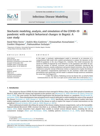
The flow diagram of the proposed mathematical model is shown in Fig. 1. Specifically, individuals transition from one
compartment to another according to specific rates and are influenced by noise, which simulates the random dynamics of the
epidemic. The model assumes that the total population is homogeneous and constant in size N. Immigration and emigration
are not taken into account; that is, the population is closed.
For this work, we introduce the following the sub-populations: Susceptible (S), Confined (C), Exposed (E), Asymptomatic
(IA), Symptomatic (IS), Quarantined (Q), Hospitalized (H), Recovered (R), and Dead (D). Susceptible individuals consist of in-
dividuals who are not infected with COVID-19 and are not isolated from the population. Confined individuals are individuals
who were previously susceptible but by their own or regulatory decision are temporarily isolated from the population in
order to protect themselves from infection. Exposed individuals are individuals who are no longer susceptible because they
have come into contact with asymptomatic or symptomatic infected individuals and are in the incubation period of disease
progression. Asymptomatic individuals are infected individuals who do not exhibit any symptoms of COVID-19, while
symptomatic individuals are infected individuals who do have symptoms. Hospitalized individuals are individuals who have
been symptomatic and enter hospitalization with severe COVID-19 symptoms. Quarantined individuals are symptomatic
individuals who have been isolated. Note that in this model, we suppose that symptomatic population immediately go to
quarantine and does not include any death of this population. However, with more available data, we could consider this case
in the future. Recovered individuals consist of individuals who were previously infectious and has now survived COVID-19.
Deceased individuals are individuals who were infectious but did not survive COVID-19. Given that, we assume a closed
population size, N ¼ S þ C þ E þ IA þ IS þ H þ Q þ R þ D.
In addition, we define the parameters used for the model in Table 1. The rates at which susceptible and confined in-
dividuals enter and leave confinement depend on the Dirac delta functions 4(t) and j(t). Susceptible individuals become
exposed upon contact with the infected population at the transmission rate b. Exposed individuals become infected at the
incubation rate, k, such that a fraction p becomes symptomatic infectious and the remaining (1 p) becomes asymptomatic
D. Ni~
no-Torres, A. Ríos-Guti
errez, V. Arunachalam et al. Infectious Disease Modelling 7 (2022) 199e211
200
3. infectious. Asymptomatic individuals either recover or develop symptoms at a rate of u, with a fraction n recovering and a
fraction (1 n) becoming symptomatic. Symptomatic individuals quarantine at a rate of x. At a rate of g, a fraction q of
quarantined individuals are hospitalized and a fraction (1 q) recover. Lastly, a proportion x of hospitalized individuals die at
a rate of aD
, while a proportion (1 x) of hospitalized individuals recover at a rate of aR
.
Next, we propose the following system of stochastic differential equations for the modified Stochastic SEIR model with
random perturbations (see (Ríos-Guti
errez et al., 2021)). Note that this model will include random perturbations of the white
noise terms satisfying the Brownian motion governed by system of stochastic differential equations. Let
n
SðtÞ; EðtÞ; IAðtÞ; ISðtÞ; QðtÞ; HðtÞ; RðtÞ; DðtÞ; CðtÞ
o
t0 be an It^
o process given by the following system of differential equations:
dSðtÞ ¼
4SðtÞ þ jCðtÞ SðtÞ~
b
IA
ðtÞ þ IS
ðtÞ
N
! #
dt
s1SðtÞIA
ðtÞ
N
dB1ðtÞ
s2SðtÞIS
ðtÞ
N
dB2ðtÞ
dEðtÞ
dt
¼ ~
bSðtÞ
IA
ðtÞ þ IS
ðtÞ
N
!
kEðtÞ
dIA
ðtÞ ¼
ð1 pÞkEðtÞ uIA
ðtÞ
dt þ
s1SðtÞIA
ðtÞ
N
dB1ðtÞ
dIS
ðtÞ ¼
pkE þ ð1 nÞuIA
ðtÞ xIS
ðtÞ
dt þ
s2SðtÞIS
ðtÞ
N
dB2ðtÞ
dQðtÞ
dt
¼ xIS
ðtÞ gQðtÞ
dHðtÞ
dt
¼ qgQðtÞ ðð1 xÞaR þ xaDÞHðtÞ
dRðtÞ
dt
¼ nuIA
ðtÞ þ ð1 qÞgQðtÞ þ ð1 xÞaRHðtÞ
dDðtÞ
dt
¼ xaDHðtÞ
dCðtÞ
dt
¼ 4SðtÞ jCðtÞ;
(1)
Fig. 1. A flow diagram of the proposed model dynamics.
D. Ni~
no-Torres, A. Ríos-Guti
errez, V. Arunachalam et al. Infectious Disease Modelling 7 (2022) 199e211
201
4. where fB1ðtÞgt0 and fB2ðtÞgt0 are two independent standard Brownian motions, and considered as generalized white noise
functionals, and the constants s1 and s2 are the intensities of the noises. We note that fB1ðtÞgt0 and fB2ðtÞgt0 are defined on
the complete probability space
U; I; fIgt0; P
satisfying the usual conditions . The functions 4 ¼ 4(t) ¼ ld(t tl) and
j ¼ j(t) ¼ md(t tm), such that:
dðt txÞ ¼
1 if t tx ¼ 0
0 if t txs0
(2)
Since the transmission rate changes according to the dynamics of the confinement or lock, then the following is proposed:
~
bðt tlÞ ¼
ð1 þ eÞb if t tl 0
b if t tl 0:
(3)
2.1. Basic reproduction number
We now briefly discuss the basic reproduction number R0, which is the expected number of secondary cases produced by a
single infection in a completely susceptible population. Using the method for the epidemic models with random perturba-
tions (Ríos-Guti
errez et al., 2021), we define the basic reproduction number as follows:
R0d
Z
∞
0
bðaÞFðaÞda; (4)
where bðaÞ is the average number of newly infected individuals (in a completely susceptible population) by an infected in-
dividual that is infectious between t ¼ 0 and t ¼ a. FðaÞ is the probability that a newly infected individual will continue
infecting others during the time interval between 0 and a. This is also called the underlying survival probability (or survival
function).
In our case, the infectivity rate when the population is completely susceptible is given by
~
b1d
b
N
þ
s1
N
B1ðtÞ
if the first infected individual is asymptomatic, or
~
b2 ¼
b
N
þ
s2
N
B2ðtÞ
Table 1
Definition of Parameters in the model.
Parameter Definition
b Transmission Rate
4 Rate at which susceptible individuals enter confinement as a function of time
j Rate at which confined individuals reenter the susceptible sub-population as a function of time
k Incubation rate
u Rate at which asymptomatic individuals become symptomatic or recover
x Rate at which symptomatic individuals enter quarantine
g Rate at which quarantined individuals become hospitalized or recover
aR Recovery rate for hospitalized individuals
aD Death rate for hospitalized individuals
p Proportion of exposed individuals that become symptomatic
q Proportion of quarantined individuals that become hospitalized
n Proportion of asymptomatic individuals that recover
x Proportion of hospitalized individuals that die
l Proportion of susceptible individuals that enter confinement at t ¼ tm
m Proportion of confined individuals that reenter the susceptible population at t ¼ tl
tl Lock-down release time (in days from t ¼ 0)
tm Lock-down time (in days from t ¼ 0)
D. Ni~
no-Torres, A. Ríos-Guti
errez, V. Arunachalam et al. Infectious Disease Modelling 7 (2022) 199e211
202
5. if the first infected individual is symptomatic. When the first infected individual infects a completely susceptible popu-
lation with N individuals, then the expected number of asymptomatic individuals who were infected by a symptomatic in-
dividual is
b1ðaÞ ¼ N~
b2ð1 pÞ ¼ ðbþ s2EðB2ðþ∞ÞÞÞð1 pÞ;
the expected number of symptomatic individuals who were infected by a symptomatic individual is
b2ðaÞ ¼ N~
b2p ¼ b þ s2EðB2ðþ∞ÞÞp;
and the expected number of asymptomatic individuals who were infected by a asymptomatic individual and have not
recovered from the illness, that is, became in symptomatic individuals is
b3ðaÞ ¼ N~
b1ð1 yÞð1 pÞ ¼ ðbþ s1EðB1ðþ∞ÞÞÞð1 yÞð1 pÞ;
and the expected number of symptomatic individuals who were infected by an asymptomatic individual is
b4ðaÞ ¼ N~
b1p ¼ b þ s1EðB1ðþ∞ÞÞp:
Note that we wrote E(Bi(þ∞)) ¼ limt/þ∞Bi(t) ¼ 1, 2 due to the need to establish how many people are infected by an
infectious individual, which we can interpret as the time of infecting from the beginning to the end of time.
In this way.
(b þ s2B2(a))p þ (b þ s2B2(a))(1 p) þ (b þ s1B1(a))(1 y)(1 p) þ (b þ s1B1(a))p
is the number of infected individuals by an infectious individual for a / þ ∞. We have the survival functions, F1(a) ¼ exa
and F2(a) ¼ eua
, for when (1) a symptomatic individual infected by a symptomatic individual remains symptomatic on [0, a],
(2) an asymptomatic individual infected by a symptomatic individual remains asymptomatic on [0, a] and (3) an asymp-
tomatic individual infected by an asymptomatic individual remains infectious on [0, a], and (4) a symptomatic individual
infected by an asymptomatic individual remains symptomatic on [0, a]; respectively. We obtain the following equation
RCov
0 d
Z
þ∞
0
bðaÞFðaÞda ¼
Z
þ∞
0
bpF1ðaÞda þ
Z
þ∞
0
bð1 pÞF2ðaÞda þ
Z
þ∞
0
bð1 yÞð1 pÞF1ðaÞda þ
Z
þ∞
0
bpF1ðaÞda
Therefore, in the following equation we introduce be(a) and Fe(a) which are functions corresponding to b(a) and F(a),
respectively, for the stochastic system (1). We then have,
Z
þ∞
0
beðaÞFeðaÞda ¼ 2
bp
x
þ
bð1 pÞ
u
þ
bð1 yÞð1 pÞ
x
þ
Z
þ∞
0
s2B2ðaÞ
pexa
þ ð1 pÞeua
da
þ
Z
þ∞
0
s1ðð1 yÞð1 pÞ þ pÞB1ðaÞexa
da: (5)
The integral
R þ∞
0 beðaÞFeðaÞda is the mean of the random variable that describes the basic reproduction number for the
proposed stochastic model. Based on (Ríos-Guti
errez et al., 2021), we have that
R1d
Z
þ∞
0
s1ðð1 yÞð1 pÞ þ pÞB1ðaÞexa
da N
0
@0;
s2
1
ð1 yÞ2
1 p
þ p
2
2x3
1
A (6)
On the other hand, using integration-by-parts rule (Chung and Williams, 2014), we have that
lim
l/þ∞
B2ðlÞðupexl
þ xð1 pÞeul
Þ ¼ B2ð0Þðpuþ ð1 pÞxÞ I1 I2 þ I3
where,
D. Ni~
no-Torres, A. Ríos-Guti
errez, V. Arunachalam et al. Infectious Disease Modelling 7 (2022) 199e211
203
6. I1 ¼
Z
þ∞
0
upxB2ðaÞexa
daI2 ¼
Z
þ∞
0
xð1 pÞuB2ðaÞeua
daI3 ¼
Z
þ∞
0
upexa
þ xð1 pÞeua
dB2ðaÞ;
We compute that liml/þ∞B2(l)(upexl
þ x(1 p)eul
) ¼ 0 a.s. In addition, B2(0) ¼ 0 a.s. Now using (Klebaner, 2012)[p. 393],
we obtain
R2 d
Z
þ∞
0
s2B2ðaÞ
pexa
þ ð1 pÞeua
da ¼
Z
þ∞
0
s2
upexa
þ xð1 pÞeua
dB2ðaÞ N 0;
s2
2ð1 pÞ2
2u3
þ
2s2
2p
1 p
ðx þ uÞxu
!
since we assumed fB1ðtÞgt0 and fB2ðtÞgt0 are two Brownian independent motions, in consequence, we get
RCov
0;v ¼
Z
þ∞
0
beðaÞFeðaÞda ¼ RCov
0 þ R2 þ R1 N
RCov
0 ; VarðR1Þ þ VarðR2Þ
: (7)
Thus, we obtain the distribution of the basic reproduction number for the proposed model.
2.2. Numerical discretization
We now briefly explain the numerical approximation method used in the paper. The Euler-Maruyama method described
in (Kloeden and Platen,1992) and introduced by the Japanese mathematician G. Maruyama (Maruyama,1955) as an extension
of the Euler method, is a numerical integration technique for obtaining approximate solutions for a system of stochastic
differential equations from a given initial value X0 ¼ x0. Let 0 ¼ t0 t1 / tk1 tk ¼ T be a partition of the interval [0, T],
where the length of each subinterval is Dt ¼ tiþ1 ti ¼ T/k, which implies that tiþ1 ¼ ti þ Dt ¼ iDt and
DBi ¼ DB(ti) ¼ B(ti þ Dt) B(ti). For each stochastic process trajectory, the value of Xtiþ1
is approximated using only the value of
the previous time step, Xti
. Then, to find the trajectories or approximate solutions of a stochastic differential equation by the
Euler-Maruyama method, the following equation is implemented:
Xtiþ1
¼ Xti
þ mðti; Xti
ÞDt þ sðti; Xti
ÞDBi (8)
for all i ¼ 0, 1, …, k 1. In order to carry out the method computationally, it is necessary to know how to calculate DBi. Since
the partition is made up of equal intervals, the differences DBi, i ¼ 0,1, …, k 1 have the same distribution, DBi ~ N(0, Dt). Let h
be a random variable with a standard normal distribution h ~ N(0,1). Then
ffiffiffiffiffiffi
Dt
p
h has a normal distribution with zero mean and
variance Dt; that is,
ffiffiffiffiffiffi
Dt
p
h Nð0;DtÞ. We use the following algorithm to implement the Euler-Maruyama method to find the
approximate solutions of the stochastic differential equations:
To implement in an analogous way the algorithm of the Euler-Maruyama method, previously described, for our proposed
model, the respective discretization of the system of stochastic differential equation (1) must be carried out, which is given
by:
D. Ni~
no-Torres, A. Ríos-Guti
errez, V. Arunachalam et al. Infectious Disease Modelling 7 (2022) 199e211
204
7. Stiþ1
¼ Sti
4Sti
jCti
þ bSti
IA
ti
þ IS
ti
N
! #
Dt
Sti
s1IA
ti
N
ffiffiffiffiffiffi
Dt
p
h1i
Sti
s2IS
ti
N
ffiffiffiffiffiffi
Dt
p
h2i
Ctiþ1
¼ Cti
þ ½4Sti
jCti
Dt
Etiþ1
¼ Eti
þ
bSti
IA
ti
þ IS
ti
N
!
kEti
#
Dt
IA
tiþ1
¼ IA
ti
þ
h
ð1 pÞkEti
uIA
ti
i
Dt þ
Sti
s1IA
ti
N
ffiffiffiffiffiffi
Dt
p
h1i
IS
tiþ1
¼ IS
ti
þ
h
pkEti
þ ð1 nÞuIA
ti
xIS
ti
i
Dt þ
Sti
s2IS
ti
N
ffiffiffiffiffiffi
Dt
p
h2i
Qtiþ1
¼ Qti
þ
h
xIS
ti
gQti
i
Dt
Htiþ1
¼ Hti
þ
qgQti
ðð1 xÞaR þ xaDÞHti
Dt
Rtiþ1
¼ Rti
þ
h
nuIA
ti
þ ð1 qÞgQti
þ ð1 xÞaRHti
i
Dt
Dtiþ1
¼ Dti
þ ½xaDHti
Dt:
(9)
3. Computational results from the statistical data: A case study from the city of Bogot
a
In this section, we discuss the stochastic dynamics with environmental noises for the COVID-19 epidemic in Bogot
a city.
The data used in this article for the simulations, parameter adjustment, and analysis was selected from the publicly available
database of the National Institute of Health of Colombia (or in Spanish: Instituto Nacional de Salud, INS) (Instituto Nacional de
Salud de Colombia, 2021). This data source provides daily case numbers for both symptomatic and asymptomatic infected
individuals without making a clear distinction between the two conditions. It also gives the report of recovered and deceased
individuals. However, given that the selected epidemiological data often had irregularities, data cleaning was performed.
Subsequently, the new database was filtered with respect to the dates of the analysis. In addition, it is necessary to have the
total number of inhabitants in the city of Bogot
a D.C. for the mathematical modelling. The population projection of the
National Administrative Department of Statistics (or in Spanish: Departamento Administrativo Nacional de Estadística, DANE)
(Administrativo Nacional de Estadística, 2018), estimates that for 2020 the total population in the respective city is 7743 955
persons. Finally, the entire methodological procedure was developed in Python 3.7.
For the proposed model (1) model, we have taken into account the first 200 days of the pandemic in the city of Bogota. The
first contagion report occurred on March 6, 2020 (Ministerio de Salud y Protecci
on Social, 2020) (day 1) and the end date of
the analysis was set for September 22, 2020 (day 200). The calibration of the model was carried out with the infected,
recovered, and deceased data of the first 100 days, that is, from March 6, 2020, to June 14, 2020 (day 100). It is planned for the
period from June 15, 2020 to September 22, 2020. The lockdown began on March 24, 2020 (Presidencia de la Repúblicade
Colombia, 2020a, 2020b) (day 18) and the partial opening began on May 11, 2020 (Presidencia de la Repúblicade Colombia,
2020a, 2020b) (day 66). By September 22, 2020, the following was reported in Colombia: 777 537 infected, 650 801 recovered,
24 570 deaths, and 3460 714 processed samples. And for the city of Bogot
a D.C, the following was reported: 256,162 infected,
213,956 recovered, and 6,610 deaths (see Table 2). Regarding the daily report of infected in the same city, its maximum value
or peak occurred around August 6, 2020, with 6068 infected cases (see Figs. 2 and 3).
3.1. Calibration of the model
The calibration of the proposed model is carried out in order to find a set of parameters so that the model has a good
description of the behavior of the system dynamics, i.e. so that the model fits the data as well as possible and allows us to
make the desired projections. The search for the parameters can be carried out by means of different optimization algorithms.
The non-linear least squares method of trust region was the one chosen (see (S
aez and Rittmann, 1992)), which will be
explained later on. Subsequently, the predictions of the model are compared with the real data available for the city of Bogot
a.
It is necessary to find the values of the parameters that fit the model according to the available data and satisfy a certain set
of constraints to ensure global convergence and consistency of the parameters. We present the nonlinear least squares
optimization method of trust region described in (Kloeden and Platen, 1992) for the adjustment of the parameters of the
proposed model. Let q ¼ (q1, …, qm) be a multidimensional parameter with a neighborhood defined by BDkðpÞ ¼ fqk2ℝ : jjpjj
Dkg for 1 k m, where Dk is the radius of the trusted region. Consider f : Rn
/R a function that depends on the parameter q.
Given some points (x1, y1)/(xn, yn) the residual sum of squares is defined as:
D. Ni~
no-Torres, A. Ríos-Guti
errez, V. Arunachalam et al. Infectious Disease Modelling 7 (2022) 199e211
205
8. gðqÞ ¼ jjy f ðx; qÞjj2
2 ¼ jjRðqÞjj2
2 (10)
where g(q) is the objective function. The information from the objective function in the trust region methods is used to form a
model mk (7), which, near the current point qk, have as much as possible a behavior similar to that of the objective function.
mkðpÞ ¼ jjRkðqkÞ þ Jkpjj2
2 (11)
where the Hessian is ▽2
g z JT
J. Since the model may not be a good approximation of the objective function, when taking
points q away from qk, the search for the minimum mk that must be restricted to points at BDk. So, in each iteration of this
methodology, the following sub-problem is solved;
min
p
mkðpÞ;
subject to jjpjj Dk.
Fig. 2. Graph (a) on left denotes number of infected individuals(incidence); Graph (b) on right denotes cumulative number of infected individuals.
Fig. 3. Graph (a) on the left denotes cumulative number of individuals recovered; Graph (b) on the right denotes cumulative number of deceased individuals.
Table 2
Statistical description of the data for the city of Bogot
a D.C
Infected Accumulated infected Recovered Accumulated recovered Dead Accumulated dead
Mean 1300.213 198 65 121.263 959 1138.063 830 42 899.111 702 36.927 374 1972.854 749
Std 1419.070 253 83 781.640 668 1593.048 383 62 834.182 549 35.517 685 2266.236 273
Min 1.000 000 1.000 000 1.000 000 1.000 000 1.000 000 1.000 000
25% 112.000 000 2390.000 000 61.250 000 1309.750 000 5.000 000 172.500 000
50% 552.000 000 16 853.000 000 372.500 000 9367.000 000 25.000 000 639.000 000
75% 2174.000 000 113 841.000 000 1734.500 000 58 568.250 000 65.500 000 3965.000 000
Max 6068.000 000 256 142.000 000 7354.000 000 213 956.000 000 122.000 000 6610.000 000
D. Ni~
no-Torres, A. Ríos-Guti
errez, V. Arunachalam et al. Infectious Disease Modelling 7 (2022) 199e211
206
9. Given the data on infected, recovered, and deceased, and the information on the parameters obtained from a meta-
analysis of the epidemiological and health entities in charge of Bogot
a, the parameters of the model were fitted with the non-
linear least squares procedure using the trust region algorithm. In Table 3 and Table 4, we can observe the fixed values and
those obtained from the model adjustment respectively, and also in the references column we can find the literature, which
helped us to establish the fixed and initial values to carry out the optimization process. Note that the standard error for the
parameters aD and x are too high, which possibly indicate that there is too much variability of the number of deaths after
COVID-19 hospitalized them: there could be days with few casualties and others with too many deaths after being hospi-
talized by COVID-19.
3.2. Model projections
Fig. 4 and Fig. 5 generally illustrate the contrast between the real dynamics and the projections of the proposed model in
the first mitigation measures for the pandemic for the SARS-CoV-2 coronavirus. Fig. 4a shows the analysis of the daily report
of individuals infected by the virus, that is, the incidence of infected. In contrast, Fig. 4b shows the analysis of the number of
accumulated infected. Fig. 5a and b represents the analysis of accumulated recovered and accumulated deceased individuals,
respectively.
In the following figures, the actual data is represented by the yellow line. The gray lines are the 20 simulations represents
results from the stochastic model subject to parameter adjustment by the trust region method, and the blue line is the drift of
the model. Likewise, the graphs specify the analysis period, that is, the period in which the parameters were projected and
adjusted. They also indicate the periods of confinement and partial opening.
Table 3
Adjusted drift parameters.
Parameter Value Units Standard error Bounds Reference
b 1.063 147 day 2.965 016 [0, 1.4] de-Camino-Beck (2020); Kumari et al. (2020)
u 0.476 190 days1
13.234 271 [1/10, 1/2.1] Mejía Becerra (2020); Imperial College London (2020)
x 0.200 000 days1
1.614 248 [1/2, 1] Harvard (2020); Belkhiria and Nascimento (2020)
aR 0.105 263 days1
6.379 961 [1/12, 1/9.5] Jafari. et al. (2021)
aD 0.131 579 days1
4.1 526Eþ2 [1/14, 1/7.6] Jafari. et al. (2021)
n 0.731 120 e 12.446 559 (0, 1) Imperial College London (2020)
x 0.900 000 e 3.1 375Eþ3 (0, 1) Imperial College London (2020)
Fig. 4. Graph (a) on left denotes number of infected individuals (incidence); Graph (b) on right denotes cumulative number of infected individuals.
Table 4
Fixed parameters.
Parameter Value Units Reference
k 1/4.6 days1
Mejía Becerra (2020); Imperial College London (2020)
g 1/8 days1
(Harvard, 2020), (Belkhiria Nascimento., 2020)
p 0.100 e Mejía Becerra (2020); He et al. (2021)
q 0.190 e Ohajunwa et al. (2020); Belkhiria and Nascimento (2020)
a 0.934 e Assumption
b 0.011 e Assumption
e 5.000 e Assumption
ta 18 days Presidencia de la Repúblicade Colombia (2020a, 2020b)
tb 66 days Presidencia de la Repúblicade Colombia (2020a, 2020b)
D. Ni~
no-Torres, A. Ríos-Guti
errez, V. Arunachalam et al. Infectious Disease Modelling 7 (2022) 199e211
207
10. The mean square logarithmic error (MSLE) is calculated as an evaluation measure of the proposed stochastic model. The
MSLE only considers the relative difference between the actual and the projected value. This measure treats minor differences
between small actual and forecasted values, roughly the same way as significant differences between large actual and
forecasted values. The cause of errors is significantly penalized than small ones in those cases where the target value range is
large. So, since the drift is the stochastic mean, when evaluated against the actual data with the MSLE measure, this gives a
cursory idea of how reliable the model is. For the projections of the incidence of infected, an MSLE of 0.090 is obtained, and for
the accumulated infected, an MSLE of 0.005, while for the predictions of accumulated recovered, an MSLE of 0.157 and for
accumulated deaths an MSLE of 0.062. Therefore, both the graphs and the superficial or general measurement of the MSLE
model infer that the projections of the recovered are not very favorable compared to the other cases.
Fig. 6 and Fig. 7 are not contrasting graphs like the previous ones. One reason could be the difficulty of obtaining the
prevalence data for the cases mentioned below. However, as can be seen, the graphs represent the 20 simulations of the
stochastic model, the drift of the model given the adjustment of the parameters and with intensity constants s1 ¼ 0.2 and
s2 ¼ 0.4 and the dates of the mitigation strategies chosen by the national government. Fig. 6a and b show possible projections
of the stochastic model for asymptomatic and symptomatic infected individuals, respectively. In contrast, Fig. 7a represent
simulations of the prevalence of hospitalized individuals, and Fig. 7b represents these changes in the stochastic dynamics of
susceptible individuals.
In our model, we obtain the basic reproduction number for the proposed model (theoretically calculated in (Ohajunwa
et al., 2020)) given by
RCov
0 ¼ b
2p
x
þ
1 p
u
þ
ð1 yÞð1 pÞ
x
Also, from the parameters given in Table 4, we note that the basic reproduction number for COVID-19 in Bogot
a has normal
distribution with median RCov
0 ¼ 4:34 and variance 1.79 (standard deviation 1.34) given by:
Fig. 5. Graph (a) on left denotes cumulative number of individuals recovered; Graph (b) on right denotes cumulative number of deceased individuals.
Fig. 6. Graph (a) on left denotes number of asymptomatic infected individuals (prevalence); Graph (b) on right denotes number of symptomatic infected in-
dividuals (prevalence).
D. Ni~
no-Torres, A. Ríos-Guti
errez, V. Arunachalam et al. Infectious Disease Modelling 7 (2022) 199e211
208
11. s2
1ðð1 yÞ2
ð1 pÞ þ pÞ2
2x3
þ
s2
2p2
2x3
þ
s2
2ð1 pÞ2
2u3
þ
2s2
2pð1 pÞ
ðx þ uÞxu
suggesting that COVID-19 could be an endemic for Bogot
a. This may also be due to the m variant B.1.621 identified in
Colombia and recognized by WHO in the list of variants that reported 25% of new incidence cases in Colombia (see (Khan
Burki, 2021; Shultzet al., 2021)).
4. Conclusion
In this work, a new stochastic epidemiological model is proposed that accounts for randomness in the dynamics of COVID-
19. The model provides a perspective of the possible scope for the spread of COVID-19 with random behaviors in the pop-
ulation. We were able to show the importance of including stochasticity within the population that models the real data from
Colombian city of Bogot
a. Our computational simulations suggest that the proposed model is reliable and robust in projecting
the number of infected, recovered and deceased individuals during interventions such as confinement and partial opening.
The results from this work can be used to inform data-driven decision making for improving public health in Colombia.
While the model seems to capture the data from the Colombian city of Bogot
a well, it is potentially limited by the lack of
prevalence data corresponding to registration of individuals who present a certain characteristic of the disease over a period
of time, including susceptible, exposed, hospitalized and quarantined sub-populations, as well as the complete registry of the
data of asymptomatic infected. The proposed model explains the containment of the pandemic by strict lock-down and
decline in number of incidence cases and death. This work also opens a way to explore newer compartment models one can
take into account including other factors such as migrations, demographics, spatial and vaccination effects. One can also
compare the proposed model against reliable data from another country. Another potential area of research includes using
these models in conjunction with machine learning and deep learning to obtain optimal parameters. Another area that can be
considered is to study to what extent the results can be generalized to the overall population and across different geographical
areas as well as patterns of contact between and within groups and in different social settings. All these will be considered in
forthcoming papers.
Availability of data and material
Not applicable. All data generated or analyzed during this study are included in this manuscript.
Funding
This work was financial support by Directorate-Bogot
a campus (DIB), Universidad Nacional de Colombia under the project
No. 50803.
Declaration of competing interest
The authors declare that they have no known competing financial interests or personal relationships that could have
appeared to influence the work reported in this paper.
Fig. 7. Graph (a) on left denotes number of people hospitalized (prevalence); Graph (b) on right denotes number of susceptible people.
D. Ni~
no-Torres, A. Ríos-Guti
errez, V. Arunachalam et al. Infectious Disease Modelling 7 (2022) 199e211
209
12. Acknowledgements
The excellent comments of the anonymous reviewers are greatly acknowledged and have helped a lot in improving the
quality of the paper.
References
de-Camino-Beck, T. (2020). A modified SEIR model with confinement and lockdown of COVID-19 for Costa Rica. In medRxiv.
Administrativo Nacional de Estadística, D. (2018). Proyecciones de poblaci
on a nivel departamental. Periodo 2018 - 2050. url: https://www.dane.gov.co/
index.php/estadisticas-por-tema/demografia-y-poblacion/proyecciones-de-poblacion.
Alberto, M., Gong, Z., Giordano, S. (2021). Modelling, prediction and design of COVID-19 lockdowns by stringency and duration. In Scientific reports, 11.1
pp. 1e13).
Amouch, M., Karim, N. (2021). Modeling the dynamic of COVID-19 with different types of transmissions. In Chaos, solitons fractals (p. 111188).
Belkhiria, Nascimento, J L. W do, Jr. (2020). COVID-19 pandemics modeling with modified determinist SEIR, social distancing, and age stratification. The
effect of vertical confinement and release in Brazil. In Plos one https://doi.org/10.1371/journal.pone.0237627. url:.
Benı
etez, M. A., et al. (2020). Responses to COVID-19 in five Latin American countries. In Health policy and technology, 9.4 pp. 525e559). https://doi.org/10.
1016/j.hlpt.2020.08.014
Brauer, F., Castillo-Chavez, C. (2012). Mathematical models in population biology and epidemiology. Springer.
Cai, S., Cai, Y., Mao, X. (2019). A stochastic differential equation SIS epidemic model with two independent Brownian motions. In Journal of mathematical
analysis and applications, 474.2 pp. 1536e1550).
C
ardenas, M., Martínez, H. (2020). COVID-19 in Colombia. Impact and Policy Responses. In Center for Global Development.
Chung, K. L., Williams, R. J. (2014). Introduction to stochastic integration. Springer.
De la Hoz-Restrepo, F., et al. (2020). Is Colombia an example of successful containment of the 2020 COVID-19 pandemic? A critical analysis of the
epidemiological data, March to july 2020. In International journal of infectious diseases (Vol. 99, pp. 522e529).
Gray, A., et al. (2011). A stochastic differential equation SIS epidemic model. In SIAM journal on applied mathematics, 71.3 pp. 876e902).
Harvard, H. U. (2020). Health Health Information and Medical Information, if you’ve been exposed to the coronavirus [Online; accessed 5-May-2021]
https://www.health.harvard.edu/diseases-and-conditions/if-youve-been-exposed-to-the-coronavirus#:#x223C;:text¼The%5C%20most%5C%20recent
%5C%20CDC%5C%20guidance,days%5C%20since%5C%20your%5C%20symptoms%5C%20began.
He, J., et al. (2021). In Proportion of asymptomatic coronavirus disease 2019: A systematic review and meta-analysis (Vol. 93, pp. 820e830). Wiley J Med Virol.
https://doi.org/10.1002/jmv.26326.
Imperial College London. (2020). MRC centre for global infectious disease analysis. url: https://mrc-ide.github.io/global-lmic-reports/parameters.html.
Instituto Nacional de Salud de Colombia. Coronavirus (COVID - 19) en Colombia. url: https://www.ins.gov.co/Noticias/Paginas/Coronaviruss.aspx.
Instituto Nacional de Salud de Colombia. (2021). Boletines casos COVID19 Colombia. url: https://www.ins.gov.co/BoletinesCasosCOVID19Colombia/Forms/
AllItems.aspx.
Jafari, Y., Rees, E. M., Nightingale, E. S. (2021). COVID-19 length of hospital stay: A systematic review and data synthesis. In BMC med (Vol. 18, p. 270).
https://doi.org/10.1186/s12916-020-01726-3
Khan Burki, T. (2021). The race between vaccination and evolution of COVID-19 variants. In The lancet respiratory medicine.
Klebaner, F. C. (2012). Introduction to stochastic calculus with applications. World Scientific Publishing Company.
Kloeden, P. E., Platen, E. (1992). Numerical solution of stochastic differential equations. Springer-Verlag Berlin Heidelberg.
Komarova, N. L., Azizi, A., Wodarz, D. (2021). Network models and the interpretation of prolonged infection plateaus in the COVID19 pandemic. In Ep-
idemics (Vol. 35, p. 100463).
Kumari, P., Singh, H. P., Singh, S. (2020). SEIAQRDT model for the spread of novel coronavirus (COVID-19): A case study in India. In Applied Intelligence.
https://doi.org/10.1007/s10489-020-01929-4
Leung, K. Y., et al. (2018). Individual preventive social distancing during an epidemic may have negative population-level outcomes. In Journal of the royal
society interface, 15.145 p. 20180296).
Lin, Q., et al. (2020). A conceptual model for the coronavirus disease 2019 (COVID-19) outbreak in Wuhan, China with individual reaction and governmental
action. In International journal of infectious diseases (Vol. 93, pp. 211e216).
Maier, B. F., Brockmann, D. (2020). Effective containment explains subexponential growth in recent confirmed COVID-19 cases in China. In Science, 368.
6492 pp. 742e746).
Maruyama, G. (1955). Continuous Markov processes and stochastic equations. In Rendiconti del Circolo Matematico di Palermo, 4.1 p. 48).
Mejía Becerra, Juan Diego (2020). In Modelaci
on Matem
atica de la Propagaci
on del SARS-CoV-2 en la Ciudad de Bogot
a Tercera Versi
on. Secretaría Distrital de
Salud de Bogot
a.
Ministerio de Salud y Protecci
on Social. (2020). Colombia confirma su primer caso de COVID-19. url: https://www.minsalud.gov.co/Paginas/Colombia-
confirma-su-primer-caso-de-COVID-19.aspx.
Musa, S. S., et al. (2021). Mathematical modeling of COVID-19 epidemic with effect of awareness programs. In Infectious disease modelling (Vol. 6, pp.
448e460).
Ohajunwa, C., Kumar, K., Seshaiyer, P. (2020). Mathematical modeling, analysis, and simulation of the COVID-19 pandemic with explicit and implicit
behavioral changes. In Computational and Mathematical Biophysics, 8 pp. 216e232). De Gruyter Open.
Oraby, T., et al. (2021). Modeling the effect of lockdown timing as a COVID-19 control measure in countries with differing social contacts. In Scientific reports,
11.1 pp. 1e13).
Prem, K., et al. (2020). The effect of control strategies to reduce social mixing on outcomes of the COVID-19 epidemic in Wuhan, China: A modelling study. In
The lancet public health (Vol. 5, p. 5). https://doi.org/10.1016/S2468-2667(20)30073-6
Presidencia de la República de Colombia. (2020a). Estas son las actividades productivas que empezar
an a reactivarse a partir del 11 de mayo, con grad-
ualidad y protocolos. url: https://id.presidencia.gov.co/Paginas/prensa/2020/Presidente-Duque-anuncia-Aislamiento-Preventivo-Obligatorio-todo-pais-
a-partir-proximo-martes-24-marzo-a-la-23-59-ho-200320.aspx.
Presidencia de la República de Colombia. (2020b). Presidente Duque anuncia Aislamiento Preventivo Obligatorio, en todo el país, a partir del pr
oximo
martes 24 de marzo, a las 23:59 horas, hasta el 13 de abril, a las cero horas. url: https://id.presidencia.gov.co/Paginas/prensa/2020/Presidente-Duque-
anuncia-Aislamiento-Preventivo-Obligatorio-todo-pais-a-partir-proximo-martes-24-marzo-a-la-23-59-ho-200320.aspx.
R
adulescu, A., Williams, C., Cavanagh, K. (2020). Management strategies in a SEIR-type model of COVID 19 community spread. In Science (Vol. 10, p. 1).
https://doi.org/10.1038/s41598-020-77628-4
Ríos-Guti
errez, A., Torres, S., Arunachalam, V. (2021). Studies on the basic reproduction number in stochastic epidemic models with random pertur-
bations. In Advances in difference equations 2021 (Vol. 1, pp. 1e24). https://doi.org/10.1186/s13662-021-03445-2
S
aez, P. B., Rittmann, B. E. (1992). Model-parameter estimation using least squares. In Water research, 26.6 pp. 789e796).
Shultz, J. M., et al. (2021). Complex correlates of Colombia's COVID-19 surge. In The lancet regional healtheamericas (Vol. 3).
Sohrabi, C., et al. (2020). World health organization declares global emergency: A review of the 2019 novel coronavirus (COVID-19). In International journal
of surgery (Vol. 76, pp. 71e76). https://doi.org/10.1016/S0140-6736(20)30185-9
D. Ni~
no-Torres, A. Ríos-Guti
errez, V. Arunachalam et al. Infectious Disease Modelling 7 (2022) 199e211
210
13. Wang, C., et al. (2020). A novel coronavirus outbreak of global health concerns. In Lancet, 395.10223 pp. 470e473). https://doi.org/10.1016/S0140-6736(20)
30185-9
World Health Organization. (March 2020). WHO Director-General’s opening remarks at the media briefing on COVID-19 - 11. https://www.who.int/director-
general/speeches/detail/who-director-general-s-opening-remarks-at-the-media-briefing-on-covid-19—11-march-2020. 2020.
Wu, J. T., Leung, K., Leung, G. M. (2020). Nowcasting and forecasting the potential domestic and international spread of the 2019-nCoV outbreak orig-
inating in Wuhan, China: A modelling study. In The lancet, 395.10225 pp. 689e697).
D. Ni~
no-Torres, A. Ríos-Guti
errez, V. Arunachalam et al. Infectious Disease Modelling 7 (2022) 199e211
211