2. Doherty and Adler 563
not affect name recognition in the second study (con-
ducted only weeks before Election Day). In addition,
consistent with some existing work, we find that the
effects of campaign mailers are short-lived. By the time
the surveys associated with the second field experiment
were conducted, the treatment effects identified in the
first field experiment had evaporated. Similarly, the fact
that the mailers stimulated intent to turn out in the second
field experiment did not translate into an increase in like-
lihood of actually turning out to vote several weeks later.
The Effects of Campaign
Communications
As we discuss below, little work has assessed the effects
of partisan direct mail. However, a voluminous literature
has examined the effects of other forms of campaign
advertising—especially television advertising. Before
continuing, it is important to note that existing work finds
evidence that the effectiveness of campaign messages can
depend substantially on the medium through which it is
conveyed (Green and Gerber 2008; Hillygus and Shields
2009). We emphasize that the findings we present below
cannot directly address ongoing debates regarding the
effects of other forms of campaign communications. That
said, given the dearth of existing work on the effects of
partisan campaign mailers, we draw on evidence from
these related literatures to clarify our contribution and
provide theoretical grounding.
Much of the existing research on the effects of cam-
paign advertising relies on observational analyses of sur-
vey data, often in concert with administrative records of
turnout behavior or information about respondents’ polit-
ical advertising environment (e.g., Krupnikov 2011).
Other research uses lab or survey experiments (e.g.,
Ansolabehere et al. 1994; Brader 2005; Schultz and
Pancer 1997). As authors of these studies acknowledge,
each of these methodological approaches is open to cri-
tiques. Researchers who use observational data to assess
campaign effects must contend with a variety of issues
related to measuring which individuals have been exposed
to which messages—a task that is complicated by sys-
tematic biases in how respondents describe their media
consumption (Stevens 2008). Others are tied to the fact
that observed campaign activities are endogenous to elec-
tion outcomes: decisions about which races to devote
resources to and what type of messaging to use are likely
to be driven by assessments of which races are winnable,
whether the candidate is an incumbent or challenger, and
a variety of other strategic judgments.1
Lab and survey experiments overcome many of the
problems that complicate observational studies by ran-
domly assigning exposure to the communication of inter-
est and obviating concerns about the communications
being strategically targeted. However, in spite of the
efforts researchers make to mask the intents of their
research designs, these studies are often criticized as lack-
ing external validity because participants are captive
recipients of treatments who are aware that they are being
studied or because the treatments used in these experi-
ments differ from the real-world communications they are
intended to parallel (Arceneaux 2010; Kinder and Palfrey
1993; McDermott 2002).
Field experiments use randomly assigned treatments
to achieve the internal validity benefits of lab experi-
ments but achieve greater external validity by treating
participants in a natural setting where they are not aware
that they are being studied and that their response to the
information they encounter is of interest to a researcher.
Although some studies find evidence that survey and lab
experiments yield substantively similar conclusions to
findings from field experiments and other research
designs (Ansolabehere, Iyengar, and Simon 1999; Falk
and Heckman 2009; Gerber et al. 2013; Valentino,
Traugott, and Hutchings 2002), others find reason to be
cautious about claims regarding the external validity of
these experiments (Barabas and Jerit 2010; Gneezy and
List 2006; Jerit, Barabas, and Clifford 2013). Specifically,
there is reason to be concerned that lab and survey experi-
ments may overstate or otherwise distort the real-world
effects of a given treatment.
A large literature has examined the effects of non-par-
tisan get-out-the-vote messages on political participation
using field experiments (Green and Gerber 2008). More
recently, some scholars have conducted field experiments
to assess the effects of other types of political communi-
cations—typically in cooperation with partisan political
organizations or interest groups (Arceneaux and
Kolodny 2009a, 2009b; Arceneaux and Nickerson 2010;
Arceneaux 2007; Gerber 2004; Gerber et al. 2011;
Loewen and Rubenson 2011; Panagopoulos and Green
2008). However, little work has leveraged the advantages
of field experiments to assess the effects of partisan mail-
ers. Indeed, we are only aware of one published field
experiment that examines the effects of campaign mailers
sent as part of a candidate’s campaign effort. That study
finds that, in the context of a municipal mayoral election,
negative mailers increase turnout by approximately 6 per-
cent over the control group (Niven 2006).
Negative versus Positive Campaign Messaging
Much of the research on campaign advertising has
focused on negative messaging. In contrast to positive
advertising, which highlights the favorable characteris-
tics and positions of the sponsoring candidate, negative
advertising is designed to draw attention to an opponent’s
unfavorable policy positions or personal characteristics.
3. 564 Political Research Quarterly 67(3)
Theories regarding the persuasive advantages (or disad-
vantages) of negative advertising pit the expectation that
negative advertising can successfully degrade voters’
evaluations of an opposing candidate against the possibil-
ity that voters dislike candidates who attack opponents—
particularly if those attacks are perceived to be
unnecessarily rude (Roese and Sande 2006).
Similarly, some posit that negative advertising demo-
bilizes voters—perhaps by leaving individuals with the
sense that there is no “good” candidate to vote for or
degrading their assessments of the integrity or civility of
the political process (e.g., Ansolabehere et al. 1994;
Finkel and Geer 1998)—while others argue that negative
advertising can increase participation by leading voters to
see the election as more important or because voters find
negative information to be particularly useful (Goldstein
and Freedman 2002; Kahneman and Tversky 1979;
Skowronski and Carlston 1989). However, to date, find-
ings regarding the effects of negative advertising have
been mixed. Ultimately, the authors of an extensive meta-
analysis conclude, “There is no consistent evidence . . .
that negative political campaigning ‘works’ in achieving
the electoral results that attackers desire . . . Nor have we
uncovered evidence that negative campaigning tends to
demobilize the electorate . . . the overall mean effect is
approximately zero” (Lau, Sigelman, and Rovner 2007,
1185–86).
Message Timing
Beyond assessing the relative effectiveness of negative
and positive campaign mailers, the studies we report
here allow us to examine whether the effects of these
messages depend on their timing. Specifically, we fielded
similar treatment regiments at two points in the general
election cycle—one early in the campaign (mid-August)
and another during the peak of the campaign season
(mid-October). There are two reasons that this variation
in timing may affect whether voters are affected by the
mailers.
First, early in a campaign cycle a given political com-
munication may face little competition for voter atten-
tion. In contrast, the marginal effect of an additional
communication in the late stages of a highly salient elec-
tion cycle may be dampened by increased competition
from other contemporaneous messages from political
opponents or candidates involved in other races. Only 40
percent of respondents in the control group in our first
experiment reported having received political mail in the
previous week. In contrast, the second experiment was
conducted later in the campaign cycle when voters were
being inundated with messages regarding high-profile
ballot initiatives, presidential and congressional candi-
dates, and an array of candidates for state-level office. In
this experiment, 83 percent of respondents in the control
group reported having received political mail in the pre-
vious week.
Second, the effectiveness of mailers may face the
problem of diminishing returns from repeated attempts
at persuading a fixed pool of voters. The state legislative
campaigns that our messages were tied to were competi-
tive, and by the time the second field experiment was
fielded, 55 percent of the potential voters who had not
been treated with a mailer recognized the Republican
candidate and 63 percent recognized the Democratic
candidate. Thus, a substantial segment of potential vot-
ers who viewed their state Senate race as worthy of con-
sideration may have already come to recognize the
candidates and, perhaps, made up their minds about
which candidate they preferred by the time they received
a treatment mailer. Taken together, these dynamics sug-
gest that the effects of campaign communication efforts
conducted late in a campaign will be weaker than those
sent earlier in the campaign cycle. Thus, overall, we
expect that—assuming we identify any treatment
effects—the effects of the treatments in the second field
experiment will tend to be weaker than those identified
in the first.
It is important to note that scholars posit that the mobi-
lizing (or demobilizing) effects of negative advertising
are driven, in large part, by the way voters respond to the
tone of political communications in general. Thus, it is
possible that exposure to political communications may
affect assessments of whether engaging in the political
process is likely to be enjoyable, even if it does not affect
attitudes about the candidates. Indeed, Krupnikov (2011)
finds that negative advertising demobilizes voters, but
only when voters encounter that negativity after they
have already made up their mind regarding which candi-
date to support. Thus, even late in the election cycle,
exposure to political advertisements may affect whether
people are inclined to take the time to go to the polls on
Election Day.
Assessing the Effects of Campaign
Mailers
We conducted two essentially identical field experiments
to compare the effects of negative and positive campaign
mailers conceived of and designed by professional politi-
cal strategists. We examine the effects of these mailers on
candidate name recognition, candidate evaluations, and
intent to turn out to vote. Given that previous findings
regarding the effects of campaign communications have
been mixed, we are agnostic in our expectations regard-
ing the nature of these effects. Instead, we rely on random
assignment to rule out potential confounds and use two-
tailed tests of statistical significance.
4. Doherty and Adler 565
As discussed above, we fielded one study relatively
early in the 2012 general election cycle and one late in the
campaign. The initial field experiment was conducted in
two state Senate districts (SD 19 and SD 26) in a battle-
ground state. The follow-up experiment included SDs 19
and 26, as well as SD 35. All three districts were thought
likely to be very competitive; the Democratic incumbents
in SDs 19 and 26 won by 2 percentage points or less in
the previous (2008) election, and there was no incumbent
running in SD 35. Prior to the election, political observers
were referring to these districts as “swing districts,” “toss
up seats,” or “battleground seats” (Hoover 2012a, 2012b),
with the newly drawn SD 35 attracting an extraordinary
amount of expenditures by outside political action com-
mittees (Crummy 2012). The margins of victory for the
winning candidates (Democratic incumbents in SDs 19
and 26, and the Republican open-seat candidate in SD 35)
ranged from 0.3 to 7.0 percent.
The campaign professionals we worked with were
interested in examining the effects of mailers on a par-
ticular population—independent likely voters (unaffili-
ated voters—those who were not formally affiliated with
a political party—and who had turned out to vote in either
the 2008 or 2010 general election).
In each study, treatment assignment was conducted at
the household level. In cases where more than one eligi-
ble registered voter (i.e., more than one independent
likely voter) lived in a given household, one individual
was randomly selected from the voter file for inclusion in
the study, and any other eligible voter within that house-
hold was dropped from the dataset.2
Our final sample for
each study consists of individuals who fall into one of
three strata: (1) individuals who our records indicate both
do not share a phone number with any other registered
voter (of any type) and do not live with any other regis-
tered voters, (2) individuals who do not share a phone
number with any other voters but do share a physical
address with other voters, and (3) likely independent vot-
ers who share both a phone number and physical address
with one other voter. For the first experiment, within each
stratum, we randomly assigned individuals in SDs 19 and
26—with equal probability—to one of three conditions: a
control condition, a negative mailer condition, or a posi-
tive mailer condition.3
Initial Field Experiment
Two identical mailers were sent (two days apart) to tar-
geted individuals in mid-August of 2012. Although these
races would ultimately be hotly contested, the organiza-
tion we worked with reported that none of the four cam-
paigns in question had begun sending out direct mail when
we conducted the first experiment. The negative mailers
attacked the Democratic candidates’ policy positions and
the purported implications of those positions. Specifically,
the mailer in each district accused the Democratic candi-
date of eagerly supporting raising taxes: “Raising taxes.
Killing jobs.” was presented in large, bold font at the top
of the front of the mailer. The back of the mailer described
the candidate with the phrase, “Likes high taxes. How
much? $4 billion!” In contrast, the positive mailer focused
on the Republican candidate’s background and policy
goals. As with the negative mailers, the positive mailers
associated with each of the two candidates were almost
identical. Each highlighted the candidate’s background
(e.g., “Husband, father, veteran”) and promised “Jobs for
[STATE], Opportunity for All, and Limited Government.”
Three days after sending out the second mailer, we
fielded interactive voice response (IVR) surveys, attempt-
ing to contact all individuals in the target population. The
IVR surveys were conducted over several days and
yielded a final response rate of 9.2 percent.4
The survey
consisted of five questions. The first two asked respon-
dents to rate each of the candidates (generally favorable
opinion, generally unfavorable opinion, never heard of
candidate, heard of but unsure; see the appendix for full
question wording). These items provide a way to measure
candidate name recognition as well as respondents’ rat-
ings of each candidate and—when compared—which
candidate (if any) the respondent preferred.
The third question asked whether the respondent
recalled receiving any campaign mail in the previous
week. The fourth question asked respondents whether
they were registered to vote in Colorado. The final ques-
tion asked respondents whether they intended to vote in
the 2012 general election. Although 1,939 individuals
provided responses to the first item in the survey, 289
respondents did not complete the entire survey. For sim-
plicity and clarity, we restrict our sample to the cases
where the individual provided responses to all five ques-
tions in the analysis that follows. We also exclude the 110
of the remaining respondents who indicated that they
were not registered to vote in Colorado as this response
suggests that the person who completed the survey was
not the targeted voter.5
These restrictions do not materi-
ally affect the findings we report. Summary statistics for
this field experiment and the field experiment described
in the next section are presented in Table S2 of the
Supplementary Analysis Document (see supplementary
material at http://prq.sagepub.com/supplemental/).
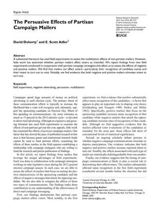
In Table 1, we estimate the effects of the mailer treat-
ments on a several outcomes of interest. We include only
indicators for treatment assignments in these models.
Including pre-treatment control variables does not affect
the substance of the findings we report here (see Table S3
in the Supplementary Analysis Document). In column 1,
we begin by examining responses to the question
that asked respondents whether they had received any
5. 566 Political Research Quarterly 67(3)
campaign mail in the previous week. The relative cam-
paign calm during this period is reflected in the fact that
only 39.4 percent of individuals in the control groups (see
coefficient on the constant) reported having received any
campaign mail at all in the previous week.6
In contrast, a
significantly larger proportion of respondents in the posi-
tive and negative mailer conditions, 57.2 and 60.2 per-
cent, respectively, reported having received mail in the
previous week (p < .01 for comparisons with control con-
dition; the difference in the proportion of respondents
reporting having received mail across the two treatment
conditions was not statistically significant, p = .266).
In this type of state-level race, campaign strategists are
often interested in two questions: whether campaign
efforts increase candidate name recognition and whether
they improve the relative standing of their candidate in
the eyes of targeted voters. Accordingly, we analyze the
effects of the mailer treatments on recognition of the can-
didates’ names. As noted above, respondents could rate
each candidate favorably, unfavorably, say they had never
heard of the candidate, or say that they had heard of the
candidate but were unsure about how they feel about the
candidate. In columns 2 and 3, we predict candidate name
recognition. Respondents who rated the candidate favor-
ably or unfavorably or said they had heard of the candi-
date but were unsure about their feelings about the
candidate are scored 1; those who had not heard of the
candidate are scored 0.7
The model in column 2 assesses the effects of the
treatments on recognition of the Republican candidate.
The constant indicates that only 17.5 percent of respon-
dents in the control condition recognized the Republican
candidate’s name. The coefficient on the Positive Mailer
Treatment indicates that this mailer—which focused
exclusively on the positive attributes of the Republican
candidate—increased the candidate’s name recognition
by 8.8 percentage points (p < .01). This amounts to a sub-
stantial proportional increase of approximately 50 per-
cent. In contrast, the Negative Mailer Treatment—which
focused exclusively on the negative characteristics of the
Democratic incumbent and did not mention the
Republican candidate by name—did not significantly
affect the Republican candidates’ name recognition.
In column 3, we see that among those in the control
group, 46.2 percent recognized the incumbent Democrat’s
name. Here the treatment effects are essentially flipped.
The Positive Mailer Treatment (which, again, did not
mention the Democratic candidate’s name) did not sig-
nificantly affect the proportion of voters who recognized
the Democratic candidate. In contrast, the Negative
Mailer Treatment increased the Democrat’s name recog-
nition by an estimated 5.9 percentage points (p < .10).
Table 1. Estimated Treatment Effects (Initial Field Experiment).
(1) (2) (3) (4) (5) (6) (7)
Yes,
received
mail
Recognize
Republican
Recognize
Democrat
Evaluation
of
Republican
Evaluation
of
Democrat
Difference in
evaluations
(Republican–
Democrat) Intent to vote
(1 = yes)
(1 = yes, 0 = no,
unsure = yes)
(1 = favorable, −1 = unfavorable,
0 = Don’t Know or never heard of)
(1 = definitely not,
4 = definitely will)
Positive Mailer Treatment 0.178***
[0.031]
0.088***
[0.026]
0.003 [0.031] 0.049**
[0.020]
−0.007
[0.034]
0.056
[0.042]
0.044
[0.035]
Negative Mailer Treatment 0.212***
[0.030]
0.003
[0.024]
0.059*
[0.031]
0.014
[0.018]
−0.033
[0.035]
0.047
[0.041]
0.080**
[0.034]
Constant 0.394***
[0.022]
0.175***
[0.017]
0.462***
[0.022]
−0.012
[0.013]
0.074***
[0.024]
−0.085***
[0.028]
3.786***
[0.026]
Observations 1,540 1,540 1,540 1,540 1,540 1,540 1,540
R2
.035 .010 .003 .004 .001 .001 .004
Positive Mailer p value .000 .001 .915 .015 .842 .186 .211
Negative Mailer p value .000 .904 .058 .457 .347 .249 .017
p value of difference
between treatments
.266 .001 .074 .085 .452 .835 .255
p value of joint significance
of treatments
.000 .001 .103 .050 .617 .343 .058
Cell entries are unstandardized OLS coefficients. Robust standard errors in brackets. OLS = ordinary least squares.
*p < .10. **p < .05. ***p < .01.
6. Doherty and Adler 567
In columns 4 to 6, we assess how the mailers affected
evaluations of the two candidates. The outcome measures
in columns 4 and 5 are scored so that those rating the
candidate favorably are scored 1, those rating the candi-
date unfavorably are scored −1, and those who either
indicated that they did not recognize the candidate or that
they were unsure how they felt about the candidate are
scored 0. The results in column 4 indicate that the Positive
Mailer Treatment had a small but statistically significant
effect on the favorability rating of the Republican candi-
date. Specifically, it increased this favorability rating by
.049 units (approximately one-fifth of a standard devia-
tion; p < .05). In contrast, the Negative Mailer Treatment
did not significantly affect ratings of the Republican can-
didate. The results in column 5 suggest that the Negative
Mailer Treatment did not significantly hurt the favorabil-
ity standing of the incumbent Democratic candidate. The
point estimates for both treatment effects are negative,
but they fall well short of conventional levels of statistical
significance both independently and jointly.
The model in column 6 estimates the effects of the
treatments on the standing of the Republican candidate
relative to the standing of the Democratic candidate mea-
sured by subtracting the Democrat’s favorability rating
from the rating of the Republican. This measure can be
interpreted as a proxy for vote preference. The evidence
suggests that the positive mailer improved the Republican
candidate’s relative standing slightly (by approximately
.056 units—about 1/10 of a standard deviation). However,
the coefficient on this treatment indicator falls short of
conventional levels of statistical significance (p = .186).
The effect of the Negative Mailer Treatment is also posi-
tive but falls short of conventional levels of statistical sig-
nificance (p = .249). The estimated effects associated
with the two treatments are statistically indistinguishable
from one another (p = .835) and the two treatment indica-
tors are not jointly significant (p = .343).
Finally, in column 7, we estimate the effects of each
treatment on responses to the intent to turn out question.
The point estimates on each treatment indicator are pos-
itive, and the coefficient on the Negative Mailer
Treatment reaches conventional levels of statistical sig-
nificance (p < .05). The coefficient on the Positive
Mailer Treatment falls short of conventional levels of
statistical significance (p = .211) but is not statistically
distinguishable from the coefficient on the Negative
Mailer Treatment (p = .255).
Follow-Up Field Experiment
The follow-up field experiment was designed to assess
whether the findings from the first field experiment rep-
licated later in the campaign cycle. The structure of the
experiment—including how the sample was identified
and which voter was sampled in households with more
than one targetable voter—mirrored the first experi-
ment. The layouts of the positive and negative mailers
used in this study were slightly different from those
used in the first field experiment, but the messaging was
virtually identical. As with the first experiment, the neg-
ative mailers highlighted the Democratic candidate’s
support for raising taxes and said the Democrat’s “bad
voting record has hurt [STATE]’s ability to build a
strong economy.” The positive mailers, again, empha-
sized positive aspects of the Republican candidate’s
background and commitment to creating jobs through
fiscally responsible policies.
This study also extended the design used in the first
field experiment in two ways. First, we included likely
independent voters from a third state Senate district
(SD 35) in the sample. Second, in addition to the posi-
tive and negative mailer treatment conditions, we
included a third treatment condition that we label the
“contrast mailer” condition. This mailer presented
information from the negative treatment mailer regard-
ing the Democratic candidate on one side and informa-
tion from the positive treatment mailer about the
Republican candidate on the opposite side. We focus
our attention on the two treatments—the positive and
negative mailer—that were comparable to those used in
the first experiment.
As with the initial experiment, treatment assignment
was done within each of the three strata described above
with targeted individuals having an equal probability of
being assigned to each of the four conditions (three treat-
ment conditions or control). For voters in SDs 19 and 26,
this treatment assignment was done independently of the
assignment in the initial experiment. Mailers were sent
out in the second week of October, 2012. Due to resource
constraints, only one mailer was sent to each targeted
individual. We attempted IVR surveys identical to those
used in the first design beginning three days after the
mailers were sent out. The surveys were conducted over
several days and yielded a final response rate of 7.0 per-
cent.8
As with the analysis presented in Table 1, we
restrict the sample to individuals who provided usable
responses to each of the five survey questions and exclude
the 5.5 percent of respondents who indicated that they
were not registered to vote.9
In Table 2, we regress each of the outcomes used in
Table 1 on indicators for each treatment condition from
the follow-up experiment, indicators for treatment
assignment from the first experiment, and—because
individuals in SD 35 were not included in the first
experiment—an indicator for respondents from this dis-
trict.10
The substantially higher intensity of campaign
activity during this period is reflected in the fact that
82.9 percent of respondents (compared with 39.1% in
7. 568 Political Research Quarterly 67(3)
the first study) who were assigned to the control condi-
tion reported having received political mail in the previ-
ous week.11
Communications during this period appear
to have been so intense that being treated with an addi-
tional mailer did not significantly affect reported receipt
of political mail (p value of test of joint significance
of treatment indicators = .901). In addition, we find
little evidence of the treatments in this experiment
affecting candidate name recognition or evaluations of
the candidate—p values associated with tests of the
joint significance of the three treatment indicators in
columns 2 to 6 range from .411 to .963.12
We do find evidence that the treatments increased
intent to turn out. Specifically, in column 7, the coeffi-
cients on the negative and positive mailer treatments each
reach conventional levels of statistical significance. The
Positive Mailer Treatment is associated with a .096 unit
increase in Intent to Vote, and the Negative Mailer
Treatment is associated with a .091 unit increase. The
coefficient on the Contrast Mailer Treatment is positive
but falls short of conventional levels of statistical signifi-
cance (p = .339).
Persistent Effects?
Finally, we assess the durability of the treatment effects
we identified in these studies. First, we examine whether
the treatment effects identified in the first study were still
observable when the second study was conducted.
Consistent with findings from recent studies that suggests
that campaign effects dissipate rapidly (e.g., Gerber et al.
2011; Hill et al. 2013), we find no evidence that the
effects identified in the first experiment were sustained
until the time of the second experiment.13
The coeffi-
cients on the treatments from the first experiment that
significantly affected outcomes in that experiment are, on
average, one-seventh of the size. The p values associated
with tests of the joint significance of the first-round treat-
ment indicators in each of the seven models fall well
short of conventional levels of statistical significance,
ranging from .487 to .958.
In addition, post-election (February 2013), we acquired
updated voter files to assess whether the effects of the
treatment mailers on reported intent to turn out in the sec-
ond study were reflected in actual turnout behavior.
Table 2. Estimated Treatment Effects (Second Field Experiment).
(1) (2) (3) (4) (5) (6) (7)
Yes,
received
mail
Recognize
Republican
Recognize
Democrat
Evaluation
of
Republican
Evaluation
of
Democrat
Difference in
evaluations
(Republican–
Democrat) Intent to vote
(1 = yes)
(1 = yes, 0 = no, unsure
= yes)
(1 = favorable, −1 = unfavorable, 0 =
Don’t Know or never heard of)
(1 = definitely not,
4 = definitely will)
Positive Mailer Treatment 0.008
[0.025]
−0.013
[0.035]
−0.008
[0.033]
0.018
[0.039]
0.002
[0.048]
0.015
[0.075]
0.096**
[0.038]
Negative Mailer Treatment 0.013
[0.026]
−0.002
[0.036]
0.028
[0.034]
0.002
[0.040]
0.064
[0.052]
−0.061
[0.077]
0.091**
[0.040]
Contrast Mailer Treatment −0.005
[0.026]
−0.016
[0.036]
−0.029
[0.034]
−0.036
[0.039]
0.002
[0.049]
−0.038
[0.075]
0.039
[0.041]
Positive Mailer Treatment
(1st round)
0.008
[0.026]
−0.009
[0.035]
−0.006
[0.034]
−0.013
[0.038]
−0.024
[0.046]
0.011
[0.070]
0.021
[0.037]
Negative Mailer Treatment
(1st round)
0.029
[0.025]
−0.009
[0.035]
0.007
[0.034]
0.032
[0.038]
−0.039
[0.048]
0.070
[0.072]
0.025
[0.037]
District 35 (1 = yes) 0.033
[0.026]
0.049
[0.036]
0.155***
[0.033]
0.049
[0.042]
−0.012
[0.052]
0.061
[0.080]
0.003
[0.040]
Constant 0.829***
[0.024]
0.550***
[0.032]
0.626***
[0.031]
0.056
[0.036]
−0.004
[0.045]
0.060
[0.069]
3.783***
[0.038]
Observations 1,552 1,552 1,552 1,552 1,552 1,552 1,552
R2
.002 .002 .020 .003 .002 .002 .006
p value of joint significance of
second-round treatments
.901 .963 .411 .582 .545 .731 .040
p value of joint significance of
first-round treatments
.487 .958 .928 .489 .712 .585 .772
Cell entries are unstandardized OLS coefficients. Robust standard errors in brackets. OLS = ordinary least squares.
*p < .10. **p < .05. ***p < .01.
8. Doherty and Adler 569
Consistent with the null effects of the first-round treat-
ments in the second-round survey, analysis of the effects
of the first- and second-round treatments on validated
turnout suggests that the mobilization effects associated
with receiving campaign mail dissipated rapidly and did
notaffectactualturnout(seeTableS8intheSupplementary
Analysis Document). We note that this null effect could
also indicate that variation in respondents’ reported intent
to turn out does not meaningfully correspond to variation
in actual participation. Although we cannot definitively
rule out this explanation, over 90 percent of respondents
who indicated that they would definitely vote did, in fact,
turn out. In contrast, only 63 percent of those who said that
they would either definitely or probably not vote actually
turned out.
Discussion
The findings we present here suggest that both positive
and negative campaign mailers can affect how voters
view the political world. Importantly, apart from their
effects on candidate name recognition, our evidence sug-
gests that the effects of negative and positive mailers are
statistically indistinguishable (for similar findings, see
Arceneaux and Nickerson 2010). Our findings also sug-
gest that the timing of these communications can have at
least two important consequences for their effectiveness.
First, the results from the first field experiment suggest
that, in the early days of the 2012 general election cycle,
the mailers increased the probability that likely indepen-
dent voters would recognize the candidate the mailer
focused on. In that experiment, we also found suggestive
evidence that the mailers improved the candidates’ elec-
toral prospects by improving their standing with voters.
In contrast, in the second field experiment, we find little
evidence that the mailers affected recipients’ assessments
or recognition of the candidates. Second, our evidence
suggests that the effect of these mailers dissipates rapidly.
We found no evidence that the effects identified in the
first treatment persisted until we fielded the second
experiment or that the effects of the treatments on intent
to turn out in the second field experiment persisted until
Election Day.14
Our evidence also supports the claim that negative
advertising—at least negative direct mail advertising—
mobilizes voters rather than demobilizing them. This is
consistent with the one previous study we are aware of
that has examined the effects of negative direct mail on
turnout (Niven 2006). Positive mailers also appear to
stimulate intent to turn out. Notably, these effects were
identified both early and late in the campaign cycle. Thus,
our findings are consistent with the claim that although
communications sent late in a campaign may be unlikely
to alter potential voters’ views about candidates, they can
affect broader assessments of the political environment
and, thereby, their eagerness to participate.15
It is important to note that, as with all research, our
evidence has limitations. First, although the mailers used
in the second field experiment contained messages that
were quite similar to those used in the first experiment,
they were not precisely identical. Second, due to resource
constraints, treated individuals in the first field experiment
received two mailers, while those in the second field
experiment received one. Given the similarities in the
effects of the treatments on intent to turn out across the
studies, we believe that the timing of the study, rather than
quantity of the treatments, is the most likely explanation
for the differences in findings across the two field experi-
ments. However, some previous studies find that treat-
ment effects associated with negative mailers are amplified
by multiple mailings (Niven 2006). In the future, research-
ers should pursue opportunities to repeat more perfectly
identical field experiments within a campaign cycle.
It is also important to note that our analysis relies on
responses from IVR surveys that yielded response rates
that, although typical for this type of survey, were none-
theless low. We did not find any statistically significant
differences between the characteristics of survey respon-
dents and non-respondents. However, we are unable to
rule out the possibility that respondents were distinctive
on unmeasured characteristics. Similarly, we cannot con-
fidently rule out the existence of complex interactions
between treatment assignment and non-response.
Other caveats to our findings stem from our successes
in achieving consistency across these studies. We focused
exclusively on estimating the effects of campaign mailers
sent on behalf of candidates from one political party. In
addition, our studies were fielded in the context of spe-
cific state legislative races during a presidential election
year. However, the effects of campaign messaging may
well vary across campaign contexts and depend on fac-
tors such as the characteristics of the candidates (e.g.,
gender, party affiliation, race), whether the campaign is
associated with a midterm, presidential, or “off-year”
election, and a range of other factors. Similarly, we
focused strictly on a target population of unaffiliated reg-
istered voters. Many unaffiliated voters—including those
who claim to be politically independent when asked—
appear to behave much like partisans (Keith et al. 1992).
However, just as we cannot definitively generalize the
treatment effects we observed among those who
responded to our surveys to those who refused, we cannot
be confident that our findings would be similar among
self-identified partisans.
These limitations aside, our findings constitute an
important contribution to our understanding of the effects
of campaign mailers. The field experiments we report
here are the first that we know of to examine the
9. 570 Political Research Quarterly 67(3)
persuasive effects of both negative and positive campaign
mailers by leveraging the advantages of random assign-
ment in a natural setting. This allows us to make clear
inference regarding the effects of the treatment mailers.
The results from two randomized field experiments dem-
onstrate that partisan campaign mailers can affect candi-
date name recognition, evaluations of candidates, and
intent to turn out. Although the effects we identified
appear to be short-lived, the findings suggest that partisan
mailers may be a valuable component of a political
campaign.
Appendix
Field Experiment Surveys Question Wording
Hello, you have been randomly selected to participate in
a brief five-question survey. This survey is for research
purposes, and we will not try to sell you anything. We
would really appreciate your participation, and your par-
ticipation and your responses will be completely
confidential.
I am going to read you the names of two individuals.
Please tell me whether you have a generally favorable or
unfavorable opinion of each one. If you have never heard
of the person, please just let us know by pressing 3. If you
have heard of the individual but are unsure about how
you feel about them, press 4.
1. What is your opinion of [REPUBLICAN
CANDIDATE NAME]?
a. Press 1 if you have a generally favorable opin-
ion of [REPUBLICAN CANDIDATE NAME]
b. Press 2 if you have a generally unfavorable of
[REPUBLICAN CANDIDATE NAME]
c. Press3ifyouhaveneverheardof[REPUBLICAN
CANDIDATE NAME]
d. Press 4 if you have heard of [REPUBLICAN
CANDIDATE NAME] but are unsure about
how you feel about them.
2. And what is your opinion of [DEMOCRATIC
CANDIDATE NAME].
a. Press 1 if you have a generally favorable opin-
ion of [DEMOCRATIC CANDIDATE NAME]
b. Press 2 if you have a generally unfavorable of
[DEMOCRATIC CANDIDATE NAME]
c. Press 3 if you have never heard of
[DEMOCRATIC CANDIDATE NAME]
d. Press 4 if you have heard of [DEMOCRATIC
CANDIDATE NAME] but are unsure about
how you feel about them.
3. Have you received any mail in the last week about
any candidates running for office in the 2012
elections?
a. Press 1 if you have received mail about the 2012
elections
b. Press 2 if you have not received mail about the
2012 elections
c. Press 3 if you are unsure
4. Are you registered to vote in [STATE]?
a. Press 1 if you are registered to vote
b. Press 2 if you are not registered to vote
c. Press 3 if you are unsure
5. How likely is it that you will vote in the 2012 elec-
tion this November: would you say you will defi-
nitely vote, probably vote, probably not vote, or
definitely not vote in the election?
a. Press 1 if you will definitely vote
b. Press 2 if you will probably vote
c. Press 3 if you will probably not vote
d. Press 4 if you will definitely not vote
Details of Field Experiment Sample
Construction
In Senate districts (SDs) 19, 26, and 35, we started with
official voter registration lists that included 101,180,
95,835, and 63,982 registered voters, respectively. We
dropped cases where an individual with the same full
name (first, middle, last names) was listed more than
once with the same phone number (SD 19 = 240 cases
dropped, SD 26 = 176, SD 35 = 94). We also, then,
dropped cases where an individual with the same full
name was listed twice at different full addresses (house
number, street name, unit number, and ZIP code; SD 19 =
32 cases, SD 26 = 32, SD 35 = 6). We also dropped any
household with more than four registered voters (SD 19 =
8,122, SD 26 = 4,591, SD 35 = 1,118). Next, because our
outcome measure is solicited via telephone calls, we
dropped any cases that did not include a phone number
(SD 19 = 14,502 cases dropped, SD 26 = 13,189, SD 35 =
10,289). We also dropped cases where individuals living
at different physical addresses were listed as having the
same phone number (SD 19 = 22,122, SD 26 = 12,075,
SD 26 = 12,075, SD 35 = 18,150).
Because our target population is likely independent
voters, we dropped all individuals who were either for-
mally affiliated with a specific political party or who
failed to vote in both the 2008 and 2010 general elections
(SD 19 = 41,693, SD 26 = 50,692, SD 35 = 28,985). In
addition, to increase the probability that our phone sur-
veys interviewed the targeted individual, we dropped
cases where individuals shared a phone number with
more than one other registered voter (SD 19 = 2,137, SD
26 = 1,805, SD 35 = 35). Treatment assignment was con-
ducted at the household level. In cases where more than
one eligible individual (i.e., more than one likely inde-
pendent voter) lived in a given household, one individual
10. Doherty and Adler 571
was randomly selected for inclusion in the study, and any
other eligible voters within that household were dropped
from the dataset.
This process yields a final sample of individuals who
fall into one of three strata. The first (stratum 1) consists
of individuals who our records indicate both do not share
a phone number with any other registered voter and do
not live with any other registered voters (SD 19 = 2,521
cases, SD 26 = 3,814 cases, SD 35 = 3,255 cases). The
second (stratum 2) includes those who do not share a
phone number with any other voters but do share a physi-
cal address with other voters (SD 19 = 3,342 cases, SD 26
= 3,736 cases, SD 35 = 1,356 cases). The third (stratum 3)
includes likely independent voters who share both a
phone number and physical address with other registered
voters but do not appear to share a phone number with
more than one other voter (SD 19 = 4,160 cases, SD 26 =
3,562 cases, SD 35 = 479 cases).
Acknowledgments
We are grateful to Kevin Arceneaux, Gregory Huber, and sev-
eral anonymous reviewers for their feedback on previous ver-
sions of this article.
Declaration of Conflicting Interests
The author(s) declared no potential conflicts of interest with
respect to the research, authorship, and/or publication of this
article.
Funding
The author(s) received no financial support for the research,
authorship, and/or publication of this article.
Notes
1. Some scholars have attempted to identify causal effects
using observational data by triangulating findings from
observational and experimental studies (Ansolabehere,
Iyengar, and Simon 1999; Lau and Pomper 2002) and using
innovative strategies like leveraging naturally occurring
discontinuities in the likelihood of exposure to advertising
(Gerber et al. 2011; Huber and Arceneaux 2007; Krasno
and Green 2008). However, it is difficult to completely
rule out problems with measurement and endogeneity in
any observational study.
2. See the appendix for further details regarding how cases in
the voter file were identified for inclusion in our sample.
3. Randomization was conducted within strata to optimize
our ability to assess whether estimated treatment effects
differed in cases where a phone number was shared or
mailers may have intercepted by another registered voter
in the household. We examined this possibility by estimat-
ing a series of regression models predicting each of the
outcomes discussed below with treatment indicators, indi-
cators for each stratum, an indicator for Senate district (SD)
26, interactions between the treatments and each of the
strata indicators, and interactions between the treatments
and the district indicator. Only in one case—recognition
of the Republican candidate’s name—did a test of the joint
significance of the strata interactions reach conventional
levels of statistical significance (p = .092). The p values
for the remaining six tests ranged from .346 to .854. Tests
of the joint significance of the district interactions all fell
short of conventional levels of statistical significance (see
Table S1 in the Supplementary Analysis Document accom-
panying the electronic version of this article at http://prq.
sagepub.com/supplemental/).
4. Response rates did not differ significantly across treatment
conditions, nor did we find evidence of differential pat-
terns of non-response across conditions associated with the
characteristics of individuals in the sample—a possibility
tested by estimating a model predicting survey participa-
tion with the strata, gender, and age of the targeted individ-
ual, indicators for each treatment, and interactions between
the treatments and strata, age, and gender (p value of test of
the joint significance of interactions = .957).
5. As expected, a regression model predicting “not regis-
tered” responses with treatment indicators was not statis-
tically significant (p = .395 for test of joint significance
of treatment indicators). A multinomial logit model pre-
dicting treatment assignment among our restricted sample
with age, gender indicators (gender is listed as unknown
for some voters), number of times the individual voted in
the last four general elections, and district did not identify
any statistically significant imbalances across treatment
conditions on these pre-treatment measures in our sample
(p value of test of joint significance of model = .736).
6. Responses of “Unsure” are treated as not having received
mail. A similar model coding those indicating hav-
ing received mail as 1, those who were unsure as 0, and
those who reported not receiving any political mail as
−1 yields similar findings (see Table S4, column 1 in the
Supplementary Analysis Document).
7. The “heard of but unsure” option was presented last
to encourage those who did not recognize the candi-
date’s name to say so rather than answering equivocally.
However, it is possible that some individuals who did not
truly recognize a candidate chose to obscure their igno-
rance by rating the candidate ambivalently. Models treat-
ing those who said they had heard of the candidate but
were unsure about how they felt about the candidate as
not recognizing the candidate (i.e., as 0s rather than 1s)
yield similar results (see Table S4, columns 2 and 3 in the
Supplementary Analysis Document).
8. Response rates did not differ significantly across treatment
conditions, nor did patterns of non-response across con-
ditions vary with the characteristics of individuals in the
sample (p value of test of the joint significance of treat-
ment × individual characteristic [strata, gender, and age]
interactions = .114).
9. As with the first experiment, a regression model predict-
ing “not registered” responses with treatment indicators
was not statistically significant (p = .821 for test of joint
11. 572 Political Research Quarterly 67(3)
significance of treatment indicators). A multinomial logit
model predicting treatment assignment with age, gender
indicators, past turnout, and district did not identify any
statistically significant imbalances across treatment con-
ditions on these pre-treatment measures in our sample (p
value of test of joint significance of model = .841). We do
not find any evidence of heterogeneity of treatment effects
(from either the first or second round of treatments) across
strata or districts (see Table S5 in the Supplementary
Analysis Document).
10. Identical analysis including a vector of pre-treatment con-
trols yields similar results to those presented in Table 2
(see Table S6 in the Supplementary Analysis Document).
11. The political organization we were working with did not
send out any other mailers about these races during or in
the two weeks prior to this second experimental period.
12. Analysis using alternative measures of recall of receiv-
ing campaign mail and candidate name recognition yields
substantively similar conclusions (see Table S7 in the
Supplementary Analysis Document).
13. In additional analysis (available upon request), we did not
find any evidence of statistically significant interactions
between the first and second round treatments.
14. We note that we are unable to determine whether the fail-
ure of the name recognition effects identified in the first
experiment to carry over to the second experiment was
due to these effects dissipating or due to a saturation effect
where most individuals in the target population had come
to recognize the candidates’ names by the time the second
experiment was fielded.
15. We note that the fact that we find that negative advertis-
ing stimulates intent to turn out late in a campaign (when
many voters may have already decided which candidate to
support) conflicts with the findings reported by Krupnikov
(2011). This divergence may stem from a variety of factors
including our focus on campaign mailers or the fact that
our sample is restricted to independents.
References
Ansolabehere, Stephen, Shanto Iyengar, and Adam Simon.
1999. “Replicating Experiments Using Aggregate and
Survey Data: The Case of Negative Advertising and
Turnout.” American Political Science Review 93:901–909.
Ansolabehere, Stephen, Shanto Iyengar, Adam Simon, and
Nicholas Valentino. 1994. “Does Attack Advertising
Demobilize the Electorate?” American Political Science
Review 88:829–38.
Arceneaux, Kevin. 2007. “I’m Asking for Your Support: The
Effects of Personally Delivered Campaign Messages on
Voting Decisions and Opinion Formation.” Quarterly
Journal of Political Science 2:43–65.
Arceneaux, Kevin. 2010. “The Benefits of Experimental
Methods for the Study of Campaign Effects.” Political
Communication 27:199–215.
Arceneaux, Kevin, and Robin Kolodny. 2009a. “Educating
the Least Informed: Group Endorsements in a Grassroots
Campaign.” American Journal of Political Science 53:
755–70.
Arceneaux, Kevin, and Robin Kolodny. 2009b. “The Effect
of Grassroots Campaigning on Issue Preferences and
Issue Salience.” Journal of Elections, Public Opinion and
Parties 19:235–49.
Arceneaux, Kevin, and David Nickerson. 2010. “Comparing
Negative and Positive Campaign Messages: Evidence
from Two Field Experiments.” American Politics Research
38:54–83.
Barabas, Jason, and Jennifer Jerit. 2010. “Are Survey
Experiments Externally Valid?” American Political
Science Review 104:226–42.
Brader, Ted. 2005. “Striking a Responsive Chord: How Political
AdsMotivateandPersuadeVotersbyAppealingtoEmotions.”
American Journal of Political Science 49:388–405.
Crummy, Karen. 2012. “Dems Ramp Up PAC Attack.” Denver
Post, October 21, 1A.
Falk, Armin, and James J. Heckman. 2009. “Lab Experiments
Are a Major Source of Knowledge in the Social Sciences.”
Science 326:535–38.
Finkel, Steven E., and John G. Geer. 1998. “A Spot Check: Casting
Doubt on the Demobilizing Effect of Attack Advertising.”
American Journal of Political Science 42:573–95.
Gerber, Alan S. 2004. “Does Campaign Spending Work? Field
Experiments Provide Evidence and Suggest New Theory.”
American Behavioral Scientist 47:541–74.
Gerber, Alan S., James G. Gimpel, Donald P. Green, and Daron
R. Shaw. 2011. “How Large and Long-Lasting Are the
Persuasive Effects of Televised Campaign Ads? Results
from a Randomized Field Experiment.” American Political
Science Review 105:135–50.
Gerber, Alan S., Gregory A. Huber, David Doherty, Conor
M. Dowling, and Costas Panagopoulos. 2013. “Big Five
Personality Traits and Responses to Persuasive Appeals:
Results from Voter Turnout Experiments.” Political
Behavior 35:687–728.
Gneezy,Uri,andJohnA.List.2006.“PuttingBehavioralEconomics
to Work: Testing for Gift Exchange in Labor Markets Using
Field Experiments.” Econometrica 74:1365–84.
Goldenberg, Edie N., and Michael W. Traugott. 1980.
“Congressional Campaign Effects on Candidate
Recognition and Evaluation.” Political Behavior 2:61–90.
Goldstein, Ken, and Paul Freedman. 2002. “Campaign
Advertising and Voter Turnout: New Evidence for a
Stimulation Effect.” The Journal of Politics 64:721–40.
Green, Donald P., and Alan S. Gerber. 2008. Get Out the Vote:
How to Increase Voter Turnout. Washington, DC: The
Brookings Institution Press.
Hill, Seth J., James Lo, Lynn Vavreck, and John Zaller.
2013. “How Quickly We Forget: The Duration Of
Persuasion Effects From Mass Communication.” Political
Communication 30 : 521-47.
Hillygus, D. Sunshine, and Todd G. Shields. 2009. The
Persuadable Voter: Wedge Issues in Presidential
Campaigns. Princeton: Princeton University Press.
Hoover, Tim. 2012a. “Hudak Fights to Keep Swing-District
Seat.” Denver Post, August 2, 5A.
Hoover, Tim. 2012b. “In Redistricted Battleground, GOP’s
Kerber Targets Newell.” Denver Post, July 7, 6A.
12. Doherty and Adler 573
Jerit, Jennifer, Jason Barabas, and Scott Clifford. 2013.
“Comparing Contemporaneous Laboratory and Field
Experiments on Media Effects.” Public Opinion Quarterly
77:256–82.
Kahneman, DanieI, and Amos Tversky. 1979. “Prospect Theory:
An Analysis of Decision Under Risk.” Econometrica
47:263–91.
Keith, Bruce E., David B. Magleby, Candice J. Nelson, Elizabeth
Orr, Mark C. Westlye, and Raymond E. Wolfinger. 1992.
The Myth of the Independent Voter. Berkeley: University
of California Press.
Kinder, Donald R., and Thomas R. Palfrey. 1993. Experimental
Foundations of Political Science. Ann Arbor: University of
Michigan Press.
Krasno, Jonathan S., and Donald P. Green. 2008. Do Televised
Presidential Ads Increase Voter Turnout? Evidence from a
Natural Experiment. Journal of Politics 70: 245-261.
Krupnikov, Yanna. 2011. “When Does Negativity Demobilize?
Tracing the Conditional Effect of Negative Campaigning
on Voter Turnout.” American Journal of Political Science
55:797–813.
Lau, Richard R., and Gerald M. Pomper. 2002. Effectiveness
of Negative Campaigning in U.S. Senate Elections.
American Journal of Political Science 46: 47-66.
Lau, Richard R., Lee Sigelman, and Ivy B. Rovner. 2007. “The
Effects of Negative Political Campaigns: A Meta-analytic
Reassessment.” The Journal of Politics 69:1176–209.
Loewen, P. John, and Daniel Rubenson. 2011. “For Want of
a Nail: Negative Persuasion in a Party Leadership Race.”
Party Politics 17:45–65.
McDermott, Rose. 2002. “Experimental Methodology in
Political Science.” Political Analysis 10:325–42.
Niven, David. 2006. “A Field Experiment on the Effects
of Negative Campaign Mail on Voter Turnout in a
Municipal Election.” Political Research Quarterly
59:203–10.
Panagopoulos, Costas, and Donald P. Green. 2008. “Field
Experiments Testing the Impact of Radio Advertisements
on Electoral Competition.” American Journal of Political
Science 52:156–68.
Roese, Neal J., and Gerald N. Sande. 2006. “Backlash Effects
in Attack Politics.” Journal of Applied Social Psychology
23:632–53.
Schultz, Cindy, and S. Mark Pancer. 1997. “Character Attacks
and Their Effects on Perceptions of Male and Female
Political Candidates.” Political Psychology 18:93–102.
Skowronski, John J., and Donal E. Carlston. 1989. “Negativity
and Extremity Biases in Impression Formation: A
Review of Explanations.” Psychological Bulletin 105:
131–42.
Stevens, Daniel. 2008. “Measuring Exposure to Political
Advertising in Surveys.” Political Behavior 30:47–72.
Stokes, Donald E., and Warren E. Miller. 1962. “Party
Government and the Saliency of Congress.” Public Opinion
Quarterly 26:531–46.
Valentino, Nicholas A., Michael W. Traugott, and Vincent L.
Hutchings. 2002. “Group Cues and Ideological Constraint:
A Replication of Political Advertising Effects Studies in
the Lab and in the Field.” Political Communication 19:
29–48.