Dissertation

An Analytical Approach to Deriving the Josephson Vortex
Solutions within Josephson Junction Containing a Single
Impurity
Christopher J. Briggs
Submitted in partial fulfilment of the requirements
for the degree of Masters of Science in Advanced Physics
at Loughborough University
September 2015
Abstract
Discussion of the applications of Terahertz (THz) Technology along with the
role in which Josephson Junctions and Vortices currently play in this
technology and the possibilities of progressing it further. An analytic
approach to deriving the Josephson relations and Sine-Gordon equation with
respect to a phase function in order to describe the behaviour of Josephson
Vortices within a homogeneous Josephson Junction. Use of a logical method
to adapt the Sine-Gordon equation and obtain a solution to describe the
behaviour of Josephson Vortices within Josephson Junctions containing a
single impurity (Inhomogeneous Josephson Junction). Brief examination of
the possible implications these Josephson Vortices may have on Terahertz
Radiation generation and modulation.
Supervisor: Professor Sergey Saveliev

I would like to dedicate this thesis
to my Parents, John and Janet Briggs,
for the love and support they have
given me my whole life to get me
to where I am today.
(Not to mention the financial cost)

Contents
1 – Introduction .......................................................................................................... 1
2 – Terahertz Technology and the Applications ......................................................... 4
2.1 – Medical Applications...................................................................................... 5
2.2 – Pharmaceutical Applications.......................................................................... 7
2.3 – Security Applications ..................................................................................... 8
2.4 – Communication and Astronomy Applications .............................................. 10
2.5 – Industrial Applications.................................................................................. 11
3 – Josephson Junctions and Vortices..................................................................... 13
3.1 – Josephson Junctions ................................................................................... 13
3.2 – Josephson Vortices ..................................................................................... 15
3.3 – Josephson Plasma Waves........................................................................... 18
3.4 – Josephson Junctions and Terahertz Technology......................................... 19
4 – Initial Plan and Objectives .................................................................................. 22
5 – Project Progression and Findings....................................................................... 26
5.1 – Josephson Relations ................................................................................... 26
5.2 – Influence of External Magnetic Field and Average Current.......................... 30
5.3 – Ferrell-Prange Equation............................................................................... 34
5.4 – Dimension and Time Adaption to Formulate Sine-Gordon Equation ........... 37
5.5 – Inhomogeneous Sine-Gordon Equation....................................................... 48
5.6 – Inhomogeneous Wave Solution................................................................... 53
5.6.1 – WKB Method......................................................................................... 53
5.6.2 – General Solution using Wave Equation................................................. 59
5.6.3 – Boundary Conditions............................................................................. 61
5.6.4 – Polylogarithm Terms ............................................................................. 63
5.6.5 – Heaviside Function................................................................................ 65
5.6.6 – Inhomogeneous Josephson Wave Solution .......................................... 69
6 – Concluding Remarks.......................................................................................... 83
Acknowledgements........................................................................................... 87
Appendix .................................................................................................................. 88
Appendix i: List of Notations ................................................................................. 88
Appendix ii: Table of Figures ................................................................................ 89
Appendix iii: References....................................................................................... 91

1
1 – Introduction
Superconductivity is a relatively young field of physics in comparison to other fields
which date back centuries; however since Heike Kamerlingh Onnes first observation
of the nature of resistance within metals that are supercooled to 4K (-269o
C), the
field has progressed exponentially. In the modern day, there are massive sums of
money being invested by leading world companies in order to discover new ways of
utilising Superconductors for application within modern world technology. From the
use of Superconductors within the Shanghai Maglev Train (fastest commercial train
in operation) which is able to send trains at speeds up to 270 mph without touching
the ground to the use within highly sensitive particle detectors, such as the Large
Hadron Collider, the applications of Superconductors could revolutionise the world.
One of the most promising applications of Superconductors is within the generation
of Terahertz radiation for use within Terahertz Technology.
Since the first postulation of a macroscopic quantum phenomenon by Brian
Josephson that explains the relationship between voltage and current within
Superconductors separated by a weak insulating barrier in 1962, there has been
great interest in the behaviour of Cooper pairs across these barriers known as
Josephson junctions. Through numerous experiments it has been proven that, within
these junctions, there exists numerous superconducting vortices (known as
Josephson vortices) propagating throughout the isolator when the superconducting
junction is placed within an external magnetic field. As a result of this discovery it
was shown that this is able to produce waves with a THz frequency. The amount of
research into the production of these THz waves as a result of the Plasma wave
mechanism within a standard Josephson junction consisting of two superconducting

2
plates and a uniform isolating layer is extensive; however research into the effect of
the impurities within this isolating layer is very limited.
This project gives a brief insight into the possible applications of Terahertz
Technology within numerous different industries, including Medical and Security
applications, and how THz waves can be produced for use within Terahertz
Technology. This also gives a short discussion as to the possible benefits of THz
frequency electromagnetic waves within these industries with consideration to
possible implications upon health, discretion, and suitability for the purpose. We will
also briefly discuss the realization of the Josephson junction, looking at some of the
other possible uses besides the generation THz radiation, and the nature of these
junctions. Following this we will discuss the formation of vortices within the isolating
layer of the Josephson junction and how these vortices interact with the Josephson
Plasma to produce Plasma waves. As a result, we will discuss how these Plasma
waves can be used to produce electromagnetic radiation and how they are used
within both generation and detection of THz radiation, with an examination of the
past research into the production of a Terahertz Imaging device.
In order to examine the influence of impurities within the Josephson junction upon
the Josephson vortices (and in turn Josephson Plasma waves and Terahertz
radiation), we will derive the Josephson relations by observing a phase function.
From there we will observe the influence of an external magnetic field and formulate
an equation which is able to describe the behaviour of the waves and vortices within
the simplest form of a Josephson junction. This will allow us to adapt the equation to
produce an equation that can explain the behaviour of waves and vortices within a
Josephson junction containing impurities. As a result we will focus our attention on
trying to analytically solve this equation, possibly using an approximation method, in

3
order to determine the impact of impurities upon vortices. The intention is to devise a
method that can be adapted for numerous impurities within a junction. By doing this,
we should be able to determine the impact that impurities has upon generating THz
radiation and whether or not it would be suitable to use this type of Josephson
junction, as oppose to the homogeneous Josephson junction, within Terahertz
Technology.

4
2 – Terahertz Technology and the Applications
In twenty-first century society technology plays a commanding role in the way in which we
live our lives on a daily basis. From medical equipment which can diagnose and treat life
threatening diseases to communications devices which can transmit a signal half way across
the world in the blink of an eye, the scientific and technological revolutions have played a
colossal role in the shaping of the modern life. However in recent years, the technology
industry has begun to undergo a Renaissance due to the relatively sudden insurgence of
Terahertz Technology. The applications and increasing benefits of using Terahertz
Technology over common methods are infinite and there has been a copious amount of
research into how it can be applied to existing technology to further improve the efficiency
and purpose of devices.
Terahertz Technology uses electromagnetic radiation with a frequency of 0.3-3THz (0.3-
3x1012
Hz) and a wave length within the submillimetre range (1x10-6
m - 1x10-3
m). These
waves are found within the terahertz gap of the electromagnetic spectrum, below
microwave radiation and above infrared radiation, which was only able to be detected
recently due to more sensitive detectors. Unlike other forms of electromagnetic radiation
with a higher frequency which is regularly used within modern technology (such as X-rays),
Terahertz Technology is non-invasive and non-destructive. However one of its most
beneficial characteristics is that it is non-ionising due to its lower photon energy, making it
very desirable within Medical and Security Technology. Another key characteristic that THz
radiation displays is its sensitivity to water; THz radiation is easily absorbed by water
molecules, allowing for determination of based on water content. Other advantageous

5
properties include its ability to easily penetrate a wide range of materials, such as plastics
and fabrics, and its spectroscopic response to many chemical compounds.
2.1 – Medical Applications
Terahertz radiation has been known for many years to be beneficial to the medical industry
due to its applications within medical imaging in comparison to current methods of imaging
the human body. Very much like X-rays, Terahertz radiation can be used to scan the inside
of the body as a result of the differences in absorption and dispersion of different types of
tissue in the body. However, the main benefit that we get from using Terahertz radiation as
oppose to X-rays, which have been common practice for many years, comes from the
differences within photon energy. X-rays characteristically have relatively high photon
energy, meaning that a patient can only be subjected to a relatively low dose of radiation
due to its ionizing effect upon biological tissue. This ionizing effect occurs as a result of the
waves interacting with atoms within tissue and removing electrons, causing the atoms to
become ionized. This can have a significant damage on the structure of DNA and cause
mutations to occur, possibly leading to formation of cancerous cells. On the other hand
Terahertz radiation has significantly lower photon energy, meaning that the waves don’t
have high enough energy to cause an ionizing effect and any possible damage is limited to
thermal effects. This means that the patient can be subjected to a higher dosage with any
hazardous effects as a result.
Terahertz radiation is also able to offer deeper penetration into tissue in order to access
biological data such as tissue density and give a better insight into the type of tissue present.
In cases where skin lesions are present, Terahertz radiation is able to be used as a diagnostic
tool in early detection of Basal Cell Carcinoma (one of the most common forms of skin

6
cancer) due to the characteristic refractive index and is able to tell the doctor about the
structural and functional information about the cancerous cells. By being able to access
tissue density as a result of water absorption, Terahertz radiation can also be used as a non-
invasive and painless method of detecting epithelial cancer. Disease detection is one of the
main focuses of Terahertz Technology within the Medical industry, and its imaging
applications go far beyond the field of Oncology. Terahertz imaging may also be used for
assessing the extent of burn damage or wound inspection without the need to remove
bandages from the victim. It may also be used to diagnose other common diseases such as
Vascular and Gastro-Intestinal diseases, giving it the edge over X-rays.
Terahertz Imaging is not just used a method of diagnosis within the medical profession; it is
also used to improve the efficiency of treatment. It can vastly improve biopsies and surgery
upon cancerous tissue within the epithelium by identifying the affected tissue more
accurately resulting in a quicker treatment time and greater chance of successfully removing
the damaged tissue before it is able to spread.
Due to the ability of Terahertz Technology to be able to distinguish the differences within
human tissue, it can be used within the field of dentistry to detect decay within teeth far
earlier than X-rays. X-rays are only able to detect decay when it reaches the surface, at
which point the treatment is limited to drilling and fillings. Whereas Terahertz Imaging can
detect tooth decay much earlier, allowing for prevention methods to be taken.
As well as the applications already discussed within the medical industry, there are
abundances of other possible uses for Terahertz Technology. It may be used to perform
label-free DNA sequencing which can be used in early diagnostic of disease, as well as being

7
a vital tool within Virology and Forensic Biology. It may also be used to assess and recognise
the presence of Protein structural states within cells.
2.2 – Pharmaceutical Applications
Within the Pharmaceutical industry it is important that the coating upon Pharmaceutical
drugs is fully intact and uniform throughout. If a drug has a non-uniform outer shell then
this can cause premature splitting and the release of high concentrations of chemicals into
the body. In order to combat this, Pharmaceutical companies use techniques of checking the
thickness of coatings in order to make that they are completely uniform. However past
techniques can cause damage the drugs, causing inaccurate testing data and leading to a
substantial financial loss as the whole batch must be destroyed if a single impurity is found
within the test samples. With the use of Terahertz radiation, it is possible to gain a more
accurate indication of the coating thickness and how long it will remain intact without
damaging or impacting upon the coating. Terahertz radiation can also tell Pharmaceutical
companies whether the drug has come into contact with water or any other substances
during tests as it is able to distinguish between different chemical compounds. As a result of
the distinguishability between different chemical compounds, Pharmaceutical companies
may use Terahertz Spectroscopy in order to produce a characteristic compound spectral
sequence in order to patent the product.
Terahertz Imaging within the body can look in depth at binding receptor conditions of cells
which is important when designing Pharmaceutical drugs that will interact with these
protein molecules in order to produce a cellular response. As well as giving cell receptor
information pre-design, it may also be used to observe the interaction with the product

8
being tested by monitoring the chemical changes within the cells, illustrating the
concentration and rate of secretion of the drug.
The use of THz radiation within the Pharmaceutical industry can revolutionise the way in
which companies can create drugs and test the efficiency and safety of their products. As
well as the discussed data that companies can gain from the use of Terahertz Technology
they can also gain other important data regarding bioavailability, manufacturability, stability,
purification, solubility and performance.
2.3 – Security Applications
One of the most promising uses of Terahertz Technology with a huge amount of money and
research being invested into it is the use within security. In a modern world with ever
growing threats to society in the form of explosives and drugs, the technology needed to be
able to detect these substances must improve at an exponential rate.
With the use of THZ radiation, it is possible for law enforcing officer to test for the presence
of explosives within a substance with great accuracy. By radiating a compound with short
pulses of THz radiation, atoms within the compound oscillate allowing for the vibrational
modes to be found for the compound. Each compound has a unique vibrational mode
pattern which acts as a fingerprint signature and through the measurement of the
vibrational mode of a compound it is possible to distinguish whether an explosive
compound is present and differentiate between chemicals to decipher what substance is
present. There is no need for law enforcers to take a sample either as the Terahertz waves
can penetrate through fabrics such as clothing in order to pick up the traces of the explosive
materials, allowing for the procedure to be carried out discretely. This process can be

9
similarly carried out to test for the presence of illegal drugs such as Methamphetamine and
is able to trace the substance even if it has been mixed with another compound designed to
disguise its presence due to the absorption peaks still being present within the spectra.
Unlike many modern scanning machines that are in use within airport security, Terahertz
Scanning machines are able to detect the presence of a weapon a lot more efficiently due to
the ability to differentiate between materials with greater success. Most scanning
equipment is only able to detect metal objects present; however with the creation of
technology such as 3D printers it is now possible to produce weapons which aren’t
detectable by this method of scanning. By using THz radiation it is possible to determine
whether someone is carrying a non-metallic weapon, such as a ceramic knife as shown in Fig
2.1. This is due to the fact that THz radiation is able to pass through clothes without being
absorbed but is absorbed by materials such as plastics and ceramics.
Fig 2.1 – Terahertz image of a man holding a concealed weapon. The weapon was made of a
ceramic material which wouldn’t have been visible using old scanning technology.
[Taken from: http://photonics.apl.washington.edu/Research.htm]

10
Due to the ability of Terahertz Technology to be able to distinguish non-metallic objects, it
can be used to find Anti-Personnel Landmines which have no metallic components as
current radar systems can’t decipher them from rocks. Due to the non-destructive and non-
invasive characteristics of THz Scanners, it is also possible to scan packages and luggage
without having to open or compromise the package. This type of technology is very
beneficial for things like airport where there is a high security threat present.
2.4 – Communication and Astronomy Applications
Despite Terahertz photons being easily absorbed by water molecules, a characteristic which
proves beneficial within medical applications of Terahertz Technology, it becomes a great
hindrance to its applications within communications devices. The use of Terahertz
Communications within the atmosphere, especially at ground level in humid climates, is not
a viable application due to the water level within the air. Terahertz waves are able to
propagate through the atmosphere over short distances without being majorly effected by
the moisture in the air; however over long distances much of the information becomes lost
due to the interaction with the water molecules. This is one of the current flaws with its use
within communication devices and there is a lot of investment from telecommunication
companies to try and rectify this problem. It is suggested that should this problem be
rectified, allowing for long distance communications with little to no data loss, Terahertz
Bandwidth could improve the speed of mobile phone devices by a factor of a thousand.
One of the current and proven applications of this technology is its use within satellite to
satellite communications. Due to the sever lack of water molecules within the exosphere,
Terahertz waves can be used to send signals without the signal becoming compromised. As
a result of the large Bandwidth Gap, massive amounts of data can be transmitted and

11
received very easily. Satellite Telescopes can also use Terahertz Technology in order to
observe interstellar chemistry as well as star formation.
2.5 – Industrial Applications
Terahertz Technology is very valuable to large industrial companies who oversee mass
chemical reactions in the production of chemical compounds for other industries. By the use
of Terahertz time domain spectroscopy, which uses optoelectronic techniques, it is possible
to subject a gaseous chemical compound with short pulse Terahertz radiation in order to
obtain results relating to its composition. By observing the unique fingerprint of chemical
composition, the technicians can acquire data relating to the molecules present and the
molar makeup. This allows for calculation of the rate of reaction within the container and
trace of transition from one dominated mixture to another without direct measurement.
Terahertz Scanning may also be used within the food production industry due to the
characteristic absorption by water molecules. The water levels within muscular parts of
meat is significantly higher than within surrounding fat layers, so when meat is scanned
using Terahertz radiation, the fat has little to no radiation absorption and is therefore
transparent upon the scan. This can tell the food companies about the fat distribution, used
in order to calculate the nutritional values of a product, as well as give an estimation for the
consume date of the product based on the amount of moisture within. This is very similar to
applications within the cosmetics industry which utilises THz radiation by examining
moisture within the skin during the testing of new skin products.
Along with all the discussed benefits and applications of Terahertz Technology, there is an
exponentially growing number of applications within the modern world; from improving

12
performance of semi-conducting and metamaterials to non-invasive examination of
priceless and fragile paintings and artefacts. Terahertz Technology is the primary cause of
one of the biggest revolutions within technology and has the power mould the technology
of the future.

13
3 – Josephson Junctions and Vortices
As we have already discussed the applications of Terahertz Technology are seemingly
endless and can prove very beneficial to mankind, however the development and utilisation
of this technology is slow due to one main factor which is holding it back. In order for the
use of Terahertz radiation within technology, we need a source that is able to produce a
steady production of Terahertz waves. Current methods of Terahertz wave generation are
not able to produce a source of intense and continuously coherent THz waves. This is the
main factor that is holding back the development of Terahertz Technology and it is thought
that one of the solutions to this is to use Josephson Junctions in order to induce the
production of THZ waves.
3.1 – Josephson Junctions
By cooling certain metals, such as lead and mercury, we are able to produce a
superconducting state in which electrons become paired together to produce Cooper pairs.
This arises as a result of the condensation of the electrons, which leaves a band gap, and can
only be described as an exchange of phonons between two coupled electrons and as a
result the electron pairs start to act boson-like. This superconducting state allows for these
Cooper pairs to move without any form of resistance, causing the material to have no
resistance and therefore allowing for a large conductance of current through it. This
phenomenon has generated a relatively young branch of physics (Superconductivity) since
its discovery in the early 20th century; however the implications are once again very
beneficial to mankind. In order to make superconductivity practical for use within the
modern world, it is important to find a superconductor which has a relatively high threshold

14
temperature (≈200 Kelvin) as it reduces the need to develop equipment to supercool the
material to very low temperatures (<20 Kelvin). By using metallic alloys and inorganic
materials made from compounds of a metal and non-metal, this superconducting behaviour
is observable at more achievable temperatures. These compounds are known as high
temperature superconductors and can have many applications within technology; from use
within fast digital circuits to the powerful superconducting electromagnets used within
Maglev Trains and Magnetic Resonance Imaging (MRI) machines. High temperature
superconductors are used within the creation of one of the most fundamental and
imperative types of superconducting junctions: Josephson Junctions.
The Josephson Junction, named after Brian Josephson who predicted that Cooper Pairs
were able to tunnel from one superconductor to another, is a special form of
Superconducting junction consisting of two Superconducting plates separated my an
isolating layer (shown in Fig 5.1). These two plates are placed sufficiently close together
with a thin isolating layer separating them, which is thin enough(usually a thickness of 30Å
or thinner) to allow for Cooper pairs to tunnel across the junction, producing a
superconducting current across the junction. Each Josephson junction has its own
characteristic critical current which depends upon the distance between the two
superconducting plates and can be thought of as a measure of the coupling strength
between the two plates which will always be greater than the thermal energy.
2𝑒𝑒𝑒
ħ
< 𝐽 𝐶 (3.1)
A Josephson junction can be thought of as a transistor due to its ability to amplify and
switch electronic signals; however Josephson junctions operate at frequencies of a scale 100
times faster than that of a transistor which makes them beneficial for use within electronic

15
circuits. Josephson Junctions are a commonly used within Quantum computing and make up
three of the most common Quantum Bits (Qubits): the Flux Qubit, the Charge Qubit, and the
Phase Qubit. The Phase Qubit, which is a current-biased Josephson junction, uses very low
temperatures to detect the quantum energy levels. The Flux Qubit’s state is determined by
the direction in which a current travels round the loop when an external flux is applied and
the Charge Qubit is able to determine its state by the presence or absence of a Cooper pair
on a superconducting island.
3.2 – Josephson Vortices
One of the common characteristics that a superconductor displays when the temperature is
cooled below the critical limit is the Meissner effect (shown in Fig 3.1). This effect describes
the ability of a Superconductor, when placed within an external magnetic field, to expel any
of the magnetic flux that penetrated it, such that no magnetic field penetrates it anymore;
however when some Superconductors (commonly Type-II Superconductors) undergo the
same process, they allow for partial penetration of the magnetic flux when the magnetic
field strength is greater than a critical field.
Fig 3.1 – Illustration of the Meissner Effect observed within Superconductors
[Taken From: https://en.wikipedia.org/wiki/Meissner_effect]

16
As a result of this magnetic flux penetration, we observe superconducting currents around a
normal core material creating vortices known as Abrikosov Vortices (as shown in Fig 3.2).
When the normal core material is pinned in position the superconductor is able to maintain
its zero resistivity whilst still allowing for the magnetic field to penetrate it. The magnetic
field around these cores comes from a local minimum within the order parameter at these
points which causes the magnetic field to be at a local maximum.
Fig 3.2 – Image showing the penetration of the Magnetic Flux lines penetrating a
Superconductor resulting in the formation of Abrikosov Vortices. The superconducting
current circulates the normal core material.
[Taken from: https://en.wikipedia.org/wiki/Macroscopic_quantum_phenomena]
A very similar phenomenon to this can be seen within Josephson junctions, known as a
Josephson vortex. Unlike an Abrikosov vortex, the Josephson vortex has its core within the
barrier between the two superconducting plates and the core is not made up of a normal
core material. The fact that Josephson vortices don’t have a normal core, means that there
is no upper critical field for the vortices to occur unlike Abrikosov vortices which only occur
above a critical magnetic field strength and below another critical field strength. The

17
Josephson vortices have no dependence upon any core material but on the nature and
formation of the Josephson junction and the isolating barrier instead. The size of a
Josephson vortex is determined by many more factors than Abrikosov vortices, such as the
strength of the applied magnetic field and the supercurrent within the adjacent
Superconductors. Each Josephson vortex has its own characteristic supercurrent, which
creates its own magnetic flux with field strength equal to a single flux quanta or fluxon.
Josephson vortices can also exist with integer half flux quanta (semifluxon) and are able to
induce the production of another Josephson vortex. When we integrate over a closed path
across the Josephson junction, we find that the net Josephson current cancels to zero; these
cycles represent the Josephson vortices within the junction as they carry no net current.
Fig 3.3 – Image showing the formation of Josephson vortices within a stacked Josephson
junctions when an external magnetic field is applied. The vortices form within the CuO2
insulating layer and don’t contain a normal core material.
[Taken from: http://jolisfukyu.tokai-sc.jaea.go.jp/fukyu/tayu/ACT03E/10/1001.htm]

18
3.3 – Josephson Plasma Waves
The Josephson vortices within a layered semiconductor play a very important role in the
generation of Josephson Plasma waves which are a source of Terahertz radiation that have
possible use within Terahertz Technology. When an external magnetic field and an external
current are applied to a layered Superconductor containing multiple Josephson vortices, the
fluxons (individual vortices) start to move within the isolating layer. The velocity of the
Josephson vortices is around a tenth of the speed of light within the medium and as a result
of the flow a voltage is induced across the junction. This produces an oscillating Josephson
current across in the same direction as the voltag, creating an AC Josephson current. The
alternating current arises as a result of the Josephson Effect when at temperatures below
the critical temperature of the superconductor. The Josephson Effect states that when two
Superconductors are arranged into a Josephson junction, a continuous electric current
appears as a result of the tunnelling of Cooper pairs across the junction. The oscillating
current reacts with the Josephson Plasma and induces the production of Josephson Plasma
waves which are able to propagate within the medium. The Josephson Plasma has a Plasma
resonance frequency and when the frequency of the oscillating current reaches this
frequency the plasma waves begin to propagate. These Josephson Plasma waves take the
form of a standard stationary wave and the propagation relation can be determined using
the Sine-Gordon equation (as shown later on).
𝜑 = 𝜑0 𝑒 𝑖𝑖𝑖+𝑖𝑖𝑖+𝑖𝑖𝑖
𝜔2
= 𝜔𝐽
2
+ 𝑐𝐽
2
(𝑘 𝑦)𝑘 𝑥
2
(3.2)

19
The Josephson Plasma waves are a composite wave of the Josephson current and the
electromagnetic waves as a result of the external field applied to it. Unlike a standard
electromagnetic wave, which displays only transverse components, the Josephson Plasma
wave has both longitudinal and transverse components. This can prove a problem when
trying to generate THz electromagnetic waves for the use within Terahertz Technology.
3.4 – Josephson Junctions and Terahertz Technology
As we discussed before, currently the main factor which is holding back the progression of
Terahertz Technology is the availability of sources of powerful continuous-wave THz
radiation; however the use of Josephson junctions may be a big step in solving this problem.
When a Josephson junction is manipulated in order to cause the flow of fluxons and in turn
generate Josephson Plasma waves within the junction, these waves may be modified in
order to convert them into Terahertz waves. These Josephson Plasma waves within the
junction are already propagating with a frequency well inside the THz range, so by stacking
many Josephson junctions on top of each other to produce an Intrinsic Josephson junction
and situating it next to a dielectric we can produce a sort of wave guide medium to produce
THz radiation. In order to produce an electromagnetic wave from the Plasma wave, that
contains both transverse and longitudinal elements, we impose electromagnetic boundary
conditions at the dielectric interface which results in an electromagnetic wave propagating
through the dielectric with a frequency within the THz range. For example, the use of
Bi2Sr2CaCu2O8+δ can be used to modulate the Josephson Plasma by working as a cavity which
is able to store the energy of a Josephson Plasma wave, which is then be emitted as THz
waves. Only a few percent of the energy of the Josephson Plasma wave is emitted in the

20
form of THz waves meaning that this is a much more sustainable method of producing THz
waves, allowing for more continuous production of intense THz radiation.
In recent years this technique for producing THz waves has been tested in the production of
a Terahertz Imaging device. The device involved the generation of continuous-wave
radiation with a frequency of 0.6THz using Josephson junctions which was then intensified
and collimated before being transmitted onto the sample. The returning wave was then
collected by using a Josephson junction which was coupled with a thin-film ring-slot antenna
as a detector, allowing for a varying voltage measured across the detector which could be
amplified and processed using a computer to produce a high resolution scan of the sample.
After testing, the equipment was able to produce an accurate scan which could be operated
at room-temperature and with very little noise. The benefits of using these high
temperature Josephson junctions over other superconducting methods for THz production
are that the equipment becomes more practical and compact due to its ability to work at
temperatures well above liquid helium which reduces the cost of cryogenic cooling of the
superconductors.
Terahertz generation and emission is just one of the possible uses that Josephson junction
can play within Terahertz Technology. Another possible use for Josephson junctions is to use
them to operate in a very similar way to photonic crystal in the filtration of THz radiation.
Photonic crystals are nanoscale structures that affect the motion of photons and trap light
within cavities or waveguides by containing periodic variations within the dielectric constant.
These crystals are used in devices where it is important to manipulate light such as in thin-
film optics. By manipulating the external magnetic field being applied to the Josephson
junction, it is possible to control the position of the vortices. As a result of this, we may

21
control the vortex density such that when a mixed frequency THz wave moves through it,
only the desired frequency is transmitted through and all other frequencies are reflected
back. This is used within the collimation of a THz wave before it is transmitted towards a
sample within THz Imaging.
Surface Josephson Plasma may be used as a method of THz radiation detection. Surface
Josephson Plasma waves have a lower resonant frequency than that of typical Josephson
Plasma waves and they are able to propagate between interfaces of dielectrics and metals.
When an incoming THz wave meets the surface it can initiate the excitation of the Surface
Josephson Plasma waves through resonance; therefore by detecting the presence and
frequency of Surface Josephson Plasma waves, we can detect the THz waves that are
incoming.
The use of Josephson junctions within the progression of Terahertz Technology could prove
a vital step in being able to develop equipment that is both practical and effective. The use
of High Temperature Superconductors within the Terahertz devices is beginning to prove
very advantageous over other Low Temperature Superconductors due to the lack of a need
to super-cool the equipment. As a result of this, equipment can be much more compact and
portable (allowing for easier use within the Security Industry) as well as cheaper due to
lower energy input for cryogenic cooling. The use of Josephson Junctions within these
Superconductors also allows for a compact solid-state source of intense continuous-wave
THz radiation, the biggest factor impeding the progression of Terahertz Technology. On top
of this, the low energy costs in the production of THz waves along with the ability to
accurately manipulate and detect THz radiation with high levels of sensitivity, has put
Josephson junction devices at the forefront of the future evolution of Terahertz Technology.

22
4 – Initial Plan and Objectives
Due to the sudden insurgence in research into Terahertz radiation and the development of
devices that are able to manipulate this radiation in order to use the electromagnetic waves
produced for real world applications, this project was designed to study use
superconducting junctions to produce and manipulate electromagnetic radiation within this
frequency band. The main focus of the research into superconducting junctions is based
around the arrangement of Josephson junctions and the way in which Terahertz waves
behave within the junctions. The initial plan for this project was to look at the Josephson
vortices that propagate within a simple Josephson junction and then use an analytical
approach to formulate a solution to the Josephson vortices that propagate within a
Josephson junction which has some form of impurity within it in order to create an
Inhomogeneous Josephson junction.
In order to do this we would first have to start with a basic Josephson junction arrangement
and derive the Josephson relations with respect to some wave function that is able to exist
across the two superconducting plates and consider how this varies with space between the
plates and evolves over time. From the results that we would obtain from doing this it
would then be possible to use classical electrodynamics in the form of Maxwell’s equation
to derive an equation which underpins the behaviour of a wave within a Josephson junction
placed within some external field. This equation can then be adapted, as it would only
explain the most basic case of the wave moving in one dimension without any time-
dependence, in order to create an equation which describes the motion of waves and
vortices within a Josephson junction with multiple spatial dimensions and time dependence.
Using this differential equation we are able to obtain mathematical representations for the

23
waves and vortices that are able propagate within a Josephson junction which depends on
position as well as time. This equation would be the main focus of the project specifically
looking at the Josephson vortices instead of the plane waves which are also able to
propagate.
Then we would substitute a basic standing wave function into the equation in order to find
the propagation relation between angular frequency and wave number from waves in this
junction. By standardising the units of the equation that we were able to formulate it would
be possible to substitute in a known function for Josephson vortices that propagate within a
standard Josephson congregation in order to check the solution and equation is valid for use
later on within the adaption of the equation. From this result we would then alter the set-up
of the Josephson junction by adding some form of impurity to the junction in order to
produce an inhomogeneous Josephson junction. This should have a substantial effect on the
types of waves and vortices that propagate within the junction so adjustment using an
analytical and mathematical approach in order to produce an equation which would be of a
similar form to the originally derived equation. This equation would involve most of the
same terms that were found within the equation for the homogeneous Josephson junction
with additional term which occur as a result of the interaction with the impurity within the
junction. Using the result of the homogenous equation, it would then be possible to simplify
the equation by considering the wave or vortex to be superposition of the original and some
new function that only has an effect over a short distance near the impurity.
In order to solve the equation for the inhomogeneous junction, it became necessary to use
a mathematical approach by means of an analytical or approximation method used within
the other fields of physics such as quantum mechanics. One of the initial propositions was to

24
use a variation of the Wentzel-Kramers-Brillouin approximation which is commonly used to
find approximate solutions to linear differential equations. When this method was unable to
generate an achievable or palpable solution to the equation, it became more appropriate to
use another method in order to solve the equation. The method that was decided upon was
the addition of a Delta function allowing for the solution to be broken down, meaning that it
was possible to solve the equation in separate regions as oppose to attempting to solve the
equation in one process over the entirety of the junction. This would generate a second
order partial differential equation very similar in nature to the wave equation with a known
condition when the space coordinate is zero, the position of the impurity within the junction.
Due to it being a hyperbolic second order partial differential, the result will be a made up of
two functions; one with a negative time component and one with a positive. In order to
solve this it is necessary to think of the solution as being either symmetric or asymmetric
about the impurity within the junction.
A plot of the result could then be carried out and compared to that of the vortices that are
seen within a standard Josephson junction with no impurities in order to analyse the types
of electromagnetic waves that can propagate as a result of this. As a result of this it should
be possible to examine whether the use of Josephson junctions of both the homogeneous
and inhomogeneous form are beneficial for the use it Terahertz technology.
The process of adapting the equation that relates to the behaviour of waves within the
junction should be expandable for junctions in which there are multiple impurities which
would be commonly seen in reality where we have multiple sheets of superconducting
materials stacked on top of each with impurities throughout in the form of atoms of another
material. The technique that was used for finding a solution to the adapted equation should

25
also be applicable to situations with multiple impurities by thinking of the wave as a
superposition of multiple functions which arise from each impurity.

26
5 – Project Progression and Findings
5.1 – Josephson Relations
By first considering a very basic set-up of a Josephson junction where we have two
superconducting plates that are separated by a different isolating material we can derive
the Josephson relations based around the concept of a wave function acting and moving
within the junction. For the sake of simplicity, we assume that the length and thickness of
each superconducting plate is relatively large in comparison to the size of the gap between
the two plates as shown in the Fig 5.1.
Fig 5.1 - Set-up of a Josephson Junction made of two superconducting plates (usually of the
same materials) separated by an isolating layer. The distance between the two
superconductors is relatively smaller in comparison to the length and thickness of the
superconductors.
We must now consider a wave function within superconductor 1 and 2, denoted by ψ1 and
ψ2 respectively, which would normally represent the movement of electrons within the two
material however when dealing with superconductors it represents the movement of
Cooper pairs. If the distance between the two superconductors is large such that the
isolating layer is relatively thick then we can consider the two superconductors to be in

27
isolation from each other. Due to this we can safely make that assumption that the wave
function within one of the superconductors has no influence upon the wave function within
the other superconductor as the distance is too large to allow for wave tunnelling to play a
major effect. This is similar to when we consider a wave function approaching a thick barrier
potential; the wave function is allowed to tunnel through the barrier however when it
reaches the other side of the potential the probability has significantly reduced because the
function decreases exponentially with distance.
Now when the two superconductors are brought closer together, such that they can no
longer be considered to be in isolation from each other, the wave functions of the two
superconductors start to interact and have an effect on each other. This comes as a result of
the tunnelling across the junction and the wave still having a significant enough probability
which allows for it to cause interference with the wave that is already propagating within
the superconductor. The tunnelling of the function represents the movement of Cooper
pairs across the junction from one superconductor to the other. It is important to use this
case, where we have wave function interaction between the plates due to tunnelling, when
deriving the Josephson relations due to the fact that when we create any form of Josephson
junction we arrange the superconductors such that Cooper pairs are able to channel across
from one side to another as this is the cause of the beneficial properties which Josephson
junctions exhibit. The first thing to consider when deriving the Josephson relations with
consideration to the wave function is the wave function evolution across the junction which
is given by equation (5.1).
𝑖ℏ
𝑑𝜓1
𝑑𝑑
= 𝑈1 𝜓1 + 𝐾𝜓2 (5.1)

28
𝑖ℏ
𝑑𝜓2
𝑑𝑑
= 𝑈2 𝜓2 + 𝐾𝜓1
In equation (5.1) U1 and U2 represent the wave energy of ψ1 and ψ2 respectively and K is
some coupling coefficient which related to the interaction between the two wave functions
in the junction. This illustrates that the evolution of each wave function across the two
plates is not only dependent upon its initial energy, which is expected, but also on the
interaction with the wave function as a result of the coupling of the wave functions. In order
to progress with the derivation of the Josephson relations, we must assign some value to
the wave energy term. In order to do this we make the assumption that midway between
the two plates, halfway through the isolating layer, the energy is zero as this means that the
values for U1 and U2 can be both represented in terms of voltage across the plates and are
opposite in sign to one another as shown in equation (5.2).
𝑈1 = −
𝑒𝑒
2
𝑈2 = +
𝑒𝑒
2 (5.2)
By substituting the values of U1 and U2 into equation (5.1), we obtain the result shown in
equation (5.3).
𝑖ℏ
𝑑𝜓1
𝑑𝑑
= −
𝑒𝑒
2
𝜓1 + 𝐾𝜓2
𝑖ℏ
𝑑𝜓2
𝑑𝑑
= +
𝑒𝑒
2
𝜓2 + 𝐾𝜓1 (5.3)
It is now necessary to express the wave function as a function of the cooper pair density n as
shown in equation (5.4). This is then substituted into equation (5.3) and the real and
imaginary parts are separated in order to express the change in Cooper pairs on both of the
superconducting plates.

29
𝜓1 = � 𝑛1 𝑒 𝑖𝜑1
𝜓2 = � 𝑛2 𝑒 𝑖𝜑2 (5.4)
In equation (5.4), φ1 and φ2 represent the phase of each wave function. Due to the
evolution of the wave function across the junction we see that there is a phase difference
across the junction.
𝜕𝑛1
𝜕𝜕
= +
2
ℏ
𝐾� 𝑛1 𝑛2 𝑠𝑠𝑠∆𝜑
𝜕𝑛2
𝜕𝜕
= −
2
ℏ
𝐾� 𝑛1 𝑛2 𝑠𝑠𝑠∆𝜑 (5.5)
As a result of the rule of conservation of Cooper pairs and from observation of equation
(5.5), we see that the change of the Cooper pair density of one of the plates must be equal
to the negative of the change of the Cooper pair density of the opposite plate. This tells us
that the Cooper pairs are allowed to leave one of the plates, causing a decrease in Cooper
pair density, and move to the opposite plate which causes that plates Cooper pair density to
increase. The importance of this is that the movement of Cooper pairs creates a
superconducting current across the two plates which acts as a way of preventing imbalance
between the two plates. This current is known as the Josephson current and arises across all
Josephson junctions when the plates are moved close enough to allow for Josephson
tunnelling.
The coefficients of the sine term within equation (5.5) have an interesting significance
within Josephson junctions. Due to the value of the coupling coefficient K depending upon
the distance of the plates and the arrangement of the junction, it dictates the influence that
one wave function causes upon the other which in turn sets the maximum rate of change of
the Cooper pair density. This means that when combined with the terms for the Cooper pair

30
density it becomes the critical current of the junction. The critical current represents the
maximum current that the junction is able to withhold. From this we can represent equation
(5.5) as equation (5.6), which is one of the Josephson relations.
𝐽 = 𝐽𝑐 𝑠𝑠𝑠∆𝜑 (5.6)
It is also possible to derive the second Josephson relation which relates the time evolution
of the phase across the junction to the voltage across the junction as illustrated in equation
(5.8). The result of equation (5.7) are added together in order to produce equation (5.8)
which is the second Josephson relation that explains the change in phase of the wave
function as a result of the voltage across the two superconducting plates. The constant
coefficient in front of the voltage is the reciprocal of the single magnetic flux quantum which
is known as the Josephson constant normally denoted by KJ.
𝜕𝜃1
𝜕𝜕
= −
𝐾
ℏ
�
𝑛2
𝑛1
𝑐𝑐𝑐𝑐 −
𝑒𝑒
2ℏ
𝜕𝜃2
𝜕𝜕
= −
𝐾
ℏ
�
𝑛1
𝑛2
𝑐𝑐𝑐𝑐 −
𝑒𝑒
2ℏ (5.7)
𝜕𝜕
𝜕𝜕
=
2𝑒
ℏ
𝑉
𝜕𝜕
𝜕𝜕
= 𝐾𝐽 𝑉 (5.8)
5.2 – Influence of External Magnetic Field and Average Current
Now that we had derived the Josephson relations by specifically looking at the evolution of
a wave function within the junction, it is important to look at the case when the junction is
placed within an external magnetic field and the effect that it has upon evolution of the
wave within the junction. In order to do this we have use the arrangement shown in Fig 5.2.

31
Fig 5.2 – Arrangement of a Josephson junction placed within an external magnetic field H.
The junction is of finite length L and the orientated such that the magnetic field acts within
the z direction.
Unlike the case discussed before where we allowed the junction to big almost infinitely long,
we are going to say that the length of the two superconducting plates is L in order to allow
us to calculate average values. The first step that we must take is to decide a point within
the junction where we can take the initial phase and for the sake of simplicity it is easiest to
say that happens at the point where x is equal to zero as shown in equation (5.9).
𝜑(0) = 𝜑0 (5.9)
By looking at electrodynamic behaviour of junctions within this sort of arrangement it is
now possible to derive a function for the average current across the junction. In order to do
this we start with the differential form of Ampère’s Circuital law, one of Maxwell’s
equations shown in equation (5.10), without the influence of a magnetic field.
∇ × 𝐻 =
4𝜋
𝑐
𝐽 (5.10)
This then gives us an equation for the magnetic field as a function of the change in phase
across within the junction as shown in equation (5.11). This function can then be used to as
an integral equation which allows us to integrate with respect to x in order to generate a
term for the phase of the wave function as a function of the external magnetic field that has
been applied to the junction.

32
𝐻 =
Φ
2𝜋𝜋
𝑑𝑑
𝑑𝑑 (5.11)
In equation (5.11), the distance between the two superconducting plates (thickness of the
isolating layer) is represented by d and the flux quantum that penetrates the junction is
given by Φ. Now by integrating the function between the limits of zero and x we obtain the
equation for phase as a function of the magnetic field and position as shown in equation
(5.12).
�
Φ
2𝜋𝜋
𝑑𝑑
𝑑𝑑
𝑥
0
𝑑𝑑 = � 𝐻
𝑥
0
𝑑𝑑
Φ
2𝜋𝜋
(𝜑(𝑥) − 𝜑0) = 𝐻𝐻
𝜑(𝑥) = 𝜑0 +
2𝜋𝜋
Φ
𝐻𝐻 (5.12)
This term for the phase shows that there is no dependence upon the length of the
superconducting plates within the junction put upon the initial phase at a point and the
strength of the magnetic field applied to the junction along with the position within the
junction. It also suggests that the phase is dependent upon the distance between the two
superconducting plates which is expected as it illustrates that the further the plates are
from each other the more time the phase has to evolve as the wave function propagates
between the two plates. By substituting equation (5.12) into equation (5.6) we get a
function which describes the superconducting current that acts between the two plates
when an external magnetic field is applied to the system.
𝐽 = 𝐽 𝐶 sin �𝜑0 +
2𝜋𝜋
𝛷
𝐻𝐻� (5.13)

33
By integrating this function over the length of the junction L, we are able to obtain an
equation which describes the average current within the junction as shown by equation
(5.14).
〈 𝐽 〉 =
1
𝐿
� 𝐽 𝐶 sin �𝜑0 +
2𝜋𝜋
𝛷
𝐻𝐻� 𝑑𝑑
𝐿
0
〈 𝐽 〉 =
𝐽 𝐶
2𝜋𝜋𝜋𝜋
2 sin �𝜑0 +
2𝜋𝜋
𝛷
𝐻𝐻� sin �−
𝜋𝜋
𝛷
𝐻𝐻� (5.14)
This integral was performed by use of the compound angle formula. In order to find the
maximum superconducting current we allow for the first sine function to be equal to one as
this is where the maximum is able to exist such that equation (5.14) can be simplified to
equation (5.15) and the result is shown in Fig 5.3.
〈 𝐽 〉 𝑚𝑚𝑚 = 𝐽 𝐶
Φ
2𝜋𝜋𝜋
sin �−
𝜋𝜋
𝛷
𝐻𝐻� (5.15)
Fig 5.3 – Plot of the maximum average superconducting current against the strength of the
external magnetic field as a function of position. This plot occurs when the first sin term is
taken to be equal to one. The pattern is very similar to that of Fraunhofer Diffraction pattern
with one large peak and each subsequent peak getting smaller.
0 1 2 3 4 5 6
<J>max
H(x)

34
This result tells us that we get a maximum superconducting current when the magnetic field
strength corresponds to an integer of half a magnetic flux quanta within the junction. This
result that we have obtained is able to be backed up by past research (Ooi et al, 2002),
which states that an increase in magnetic field by a half integer of the flux quanta would
result in one Josephson vortex being added per to layers.
5.3 – Ferrell-Prange Equation
In order to describe the way in which vortices and waves propagate through a Josephson
junction of any form, whether it is homogeneous or inhomogeneous, we must first try to
define some equation that is able to explain the behaviour for all waves and vortices within
a Josephson junction. To do this we are again going to start with the very most basic form of
a Josephson junction placed within an external magnetic field as shown in Fig 5.2.
However this time we are going to define the direction in which the current and the
magnetic field move by vector components as shown in equation (5.16). We do this in order
to be able to perform the curl function again using the Ampère’s Circuital Law, equation
(5.10). We are using this form of the equation as oppose to the whole equation as we are
looking for the very most basic equation to explain the behaviour of the waves and vortices
without any time dependence.
𝐻 = �
𝐻 𝑥
𝐻 𝑦
𝐻𝑧
� = �
0
0
𝐻
�
𝐽 = �
𝐽𝑥
𝐽 𝑦
𝐽𝑧
� = �
0
𝐽𝑐 𝑠𝑠𝑠𝑠
0
�
(5.16)

35
By replacing the function for H with equation (5.11) which described the magnetic field
strength as function of the phase of the wave function, we can substitute this into equation
(5.10) in order to generate a second order differential equation as shown in equation (5.17).
This is an important equation as it is one of the criteria of the waves and vortices which
operate within the junction.
𝑑
𝑑𝑑
�
Φ
2𝜋𝜋
𝑑𝑑
𝑑𝑑
� = 𝑗𝑐 sin 𝜑
𝑑2
𝜑
𝑑𝑑2
=
2𝜋𝜋
Φ
𝑗 𝐶 sin 𝜑 (5.17)
This result is a very important one within Josephson junctions as this is the most basic time-
independent version of the sine-Gordon equation which defines all waves within any form
of Josephson junction. As we know that the distance between the superconducting plates,
magnetic flux quanta and the critical current are all considered to be constants for each
Josephson junction arrangement we can replace them with a new constant. This constant is
known as the Josephson penetration depth λJ which has important significance for a
Josephson junction and is related to the setup of the junction. The Josephson penetration
depth is define by equation (5.18) and characterises the depth to which an external
magnetic field is able to penetrate into the long Josephson junction as shown by Fig 5.4.
𝜆𝐽 = �
Φ
2𝜋𝜋𝑗 𝐶 (5.18)

36
Fig 5.4 – Illustration of the penetration depth within a Josephson junction. The external
magnetic field is able to penetrate into the junction to this depth.
By substituting this term for the penetration depth into equation (5.17) we have successfully
been able to derive the Ferrell-Prange equation shown in equation (5.19) which is a
simplified one dimensional time independent version of the Sine-Gordon equation.
𝑑2
𝜑
𝑑𝑑2
=
1
𝜆𝐽
2 sin 𝜑
(5.19)
This equation is able to tell us about the dispersion relation of the waves within the junction
which outlines the necessary conditions that a wave must meet in order to be able to act
within the junction. From this we know that waves that can propagate within the junction
are of the form shown in equation (5.20).
𝜑 ≈ 𝑒
𝑥
𝜆 𝐽 (5.20)
When we have a constant Magnetic field (i.e. when there is no screening from the magnetic
field produced by the Josephson current), the solutions to the vortices take the form of a
simple sinusoidal wave moving through the junction. When we consider the case where the
magnetic field is no longer classed as being constant, such as when the magnetic field from
the Josephson current is no longer classed as negligible and causes screening, the vortices

37
take a soliton solution. We can check this solution and the equation by implementing the
soliton function that is already known for a Josephson vortex within one dimension, shown
by equation (5.21). By substituting equation (5.21) into equation (5.19), we prove that both
sides are equal (as shown in equation (5.22)) which proves the Ferrell-Prange equation and
that these vortices can propagate within this junction.
𝜑 = 4 arctan �𝑒
±
𝑥
𝜆 𝐽�
(5.21)
𝜕2
𝜕𝑥2
�4 arctan �𝑒
±
𝑥
𝜆 𝐽�� =
1
𝜆𝐽
2 sin �4 arctan �𝑒
±
𝑥
𝜆 𝐽��
𝜕2
𝜕𝑥2
�4 arctan �𝑒
±
𝑥
𝜆 𝐽�� = −
4𝑒
𝑥
𝜆 𝐽 �𝑒
2𝑥
𝜆 𝐽 − 1�
𝜆𝐽
2
�𝑒
2𝑥
𝜆 𝐽 + 1�
2
sin �4 arctan �𝑒
±
𝑥
𝜆 𝐽�� = −
4𝑒
𝑥
𝜆 𝐽 �𝑒
2𝑥
𝜆 𝐽 − 1�
�𝑒
2𝑥
𝜆 𝐽 + 1�
2
∴
𝑑2
𝜑
𝑑𝑑2
=
1
𝜆𝐽
2 sin 𝜑
(5.22)
5.4 – Dimension and Time Adaption to Formulate Sine-Gordon Equation
Despite the Ferrell-Prange equation being able to describe the one dimensional behaviour
of a wave function within the Josephson junction, it is unable to describe higher dimensional
behaviour and any time dependence behaviour of the waves. It is for this reason why we do
not commonly use this equation to describe the motion of vortices, instead we adapt upon
this equation to create the Sine-Gordon equation.

38
In order to do such a thing, we need to consider a term that is able to describe the
acceleration of vortices and waves within the junction. The reason for this is that when we
control the Josephson vortices within a Josephson junction by causing them to accelerate
and decelerate we can manipulate the plasma waves that are moving within the junction.
This is a key concept to consider when thinking about the use of this type of junction within
technology as it is what allows for the manipulation of the Terahertz radiation that is being
produced. In order to do this we can again use Maxwell’s relations, however this time we
take the version that explains behaviour within matter and we include the term that
includes the change in displacement field as shown in equation (5.23) where D represents
the displacement field.
∇ × 𝐻 = 𝐽 +
𝜕𝜕
𝜕𝜕 (5.23)
By following the same process as shown for the Ferrell-Prange equation however
considering a second special dimension when looking at the curl of the magnetic field, we
are able to derive the Sine-Gordon equation as shown in equation (5.24).
�
𝑑2
𝑑𝑑2
+
𝑑2
𝑑𝑑2
−
1
𝑐2
𝑑2
𝑑𝑑2
� 𝜑 =
sin 𝜑
𝜆𝐽
2
(5.24)
This is the most important equation that we have to consider when trying to describe the
behaviour and propagation of both vortices and waves within Josephson junctions because
in order for something to propagate in the region between the two superconducting plates
its must satisfy this condition. As we can see from equation (5.24), if the time dependence
of the wave or vortices and the one of the position dependences is zero then the equation
can be simplified down to the Ferrell-Prange equation once more.

39
In order to use this equation to check the dispersion relation of a standing wave within the
junction we must first convert equation (5.24) into standardised units in order to substitute
in a wave function. To do this, we start by introducing new variables for the position
variables which are multiplied by the Josephson penetration depth, as shown in equation
(5.25), which allows for the cancellation of the penetration depth term on the left hand side
as displayed in equation (5.26).
𝑥� =
𝑥
𝜆𝐽
𝑦� =
𝑦
𝜆𝐽 (5.25)
�
𝑑2
𝑑𝑥�2
+
𝑑2
𝑑𝑦�2
−
𝜆𝐽
2
𝑐2
𝑑2
𝑑𝑑2
� 𝜑 = sin 𝜑
(5.26)
In order to replace the time variable we must first address the coefficient of the second
order time derivative. Using the relationship expressed in equation (5.27), we are able to
replace the coefficient with a term that includes the plasma frequency of the wave within
the junction ωp.
𝜆𝐽
2
𝑐2
= 𝜔 𝑝
2
(5.27)
�
𝑑2
𝑑𝑥�2
+
𝑑2
𝑑𝑦�2
−
1
𝜔 𝑝
2
𝑑2
𝑑𝑑2
� 𝜑 = sin 𝜑
(5.28)
Now with the introduction of a new time variable as a function of the plasma frequency,
equation (5.29), we get the standardised version of the Sine-Gordon equation (equation
(5.30)) which we can use to check the dispersion relation of a Plasma wave within the
Josephson junction.
𝑡̃ = 𝜔 𝑝 𝑡 (5.29)

40
�
𝑑2
𝑑𝑥�2
+
𝑑2
𝑑𝑦�2
−
𝑑2
𝑑𝑡̃2
� 𝜑 = sin 𝜑
(5.30)
Now we will use a standard standing wave, shown in equation (5.31), to calculate the
dispersion relation between the wave number and the angular frequency of a wave within
the Josephson junction. We will do this by substituting it into equation (5.30), and
simplifying to get the angular frequency as a function of the wave number. In order to do
this we must make the assumption that the phase is suffieciently small such that the sine
function can be approximated to be equal to the phase (as shown in equation (5.32))
𝜑 = 𝜑0 𝑒 𝑖𝑖𝑖+𝑖𝑖𝑖+𝑖𝑖𝑖 (5.31)
sin�𝜑0 𝑒 𝑖𝑖𝑖+𝑖𝑖𝑖+𝑖𝑖𝑖
� ≈ 𝜑0 𝑒 𝑖𝑖𝑖+𝑖𝑖𝑖+𝑖𝑖𝑖
(5.32)
𝑑2
𝜑
𝑑𝑥�2
= −𝑘 𝑥
2
𝜑0 𝑒 𝑖𝑖𝑖+𝑖𝑖𝑖+𝑖𝑖𝑖
𝑑2
𝜑
𝑑𝑦�2
= −𝑘 𝑦
2
𝑑2
𝜑
𝑑𝑡̃2
= −𝜔2
(5.33)
𝜔 = �1 + 𝑘2 (5.34)
The relationship between the angular frequency and the wave number (equation (5.34))
holds for all electromagnetic waves that are propagating within the Josephson junction and
this is shown in Fig 5.5. These waves play a big role in the technology of tomorrow due to
the frequency characteristics as they are commonly found to be within the Terahertz range
of the electromagnetic spectrum.

41
Fig 5.5 – Dispersion relation between the angular frequency and the wave number of the
electromagnetic waves within a standard Josephson junction. The frequency of the waves is
within the Terahertz range of the electromagnetic spectrum.
Now we will prove that the function for the Josephson vortices holds for the Sine-Gordon
equation and that they can circulate within the Josephson junction. First we are going to use
a different representation to the very most basic Josephson vortex form, as discussed in
equation (5.21), which is invariant under Lorentz transformation which is represented in
equation (5.35).
𝜑 = 4 arctan �𝑒
𝑥−𝑣𝑣
√1−𝑣2
�
(5.35)
We use this equation as the vortices within the junction have the ability to move around
and the effect of the velocity can play effect on the outcome of the result for both the phase
and field of the vortices. Typically the vortices move with a velocity around 0.1 of the speed
of light in the medium. In order to prove this is a tangible solution to the Sine-Gordon we
have to substitute it into equation (5.30) and check that both sides are equal. For this
example we are not going to consider a second position dimension; we will only look at a
single position and time dependence for the vortex.

42
�
𝑑2
𝑑𝑥�2
−
𝑑2
𝑑𝑡̃2
� �4 arctan �𝑒
𝑥−𝑣𝑣
√1−𝑣2
� � = sin �4 arctan �𝑒
𝑥−𝑣𝑣
√1−𝑣2
� �
(5.36)
Unlike before we cannot say the phase is sufficiently small such that the sine of the phase
function can be approximated to be equal to the phase. To solve this it is important to
simplify the sine function using the compound angle formula in order to get a function of
just the exponent part of the vortex.
sin �4 𝑎𝑎𝑎𝑎𝑎𝑎 �𝑒
𝑥−𝑣𝑣
√1−𝑣2
�� = sin(4𝛽)
𝛽 = arctan �𝑒
𝑥−𝑣𝑣
√1−𝑣2
�
= 2 sin(2𝛽) cos(2𝛽)
= 2(2 sin(𝛽) cos(𝛽)) (2𝑐𝑐𝑐2(𝛽) − 1) (5.37)
When we now place the function for beta into the functions of sine and cosine, we obtain
an exponential function which is the result we were aiming for. For the sake of simplicity
and to make it aesthetically pleasing, the exponential terms have been replaced by Θ in
equation (5.38).
𝜃 = 𝑒
𝑥−𝑣𝑣
√1−𝑣2
sin �4 𝑎𝑎𝑎𝑎𝑎𝑎 �𝑒
𝑥−𝑣𝑣
√1−𝑣2
�� =
4(𝜃 − 𝜃3
)
(𝜃2 + 1)2 (5.38)
With this function now simplified into a form that will be easier to check whether it can be a
solution to the Sine-Gordon equation. Now we must calculate the second order derivatives
of the vortex with respect to both position and time.
𝑑𝑑
𝑑𝑑
=
4𝜃
√1 − 𝑣2 (𝜃2 + 1) (5.39)

43
𝑑2
𝜑
𝑑𝑑2
= 4 �
𝜃
(1 − 𝑣2)(𝜃2 + 1)
−
2𝜃3
(1 − 𝑣2)(𝜃2 + 1)2
�
𝑑𝑑
𝑑𝑑
=
4𝑣𝑣
𝜆𝐽√1 − 𝑣2 (𝜃2 + 1)
𝑑2
𝜑
𝑑𝑑2
= 4 �
𝑣2
𝜃
(1 − 𝑣2)(𝜃2 + 1)
−
2𝑣2
𝜃3
(1 − 𝑣2)(𝜃2 + 1)2
�
(5.40)
By using the functions that we obtained in equations (5.38), (5.39), and (5.40), we are able
to check that the wave function for the Josephson vortices is a solution by making sure that
the equation is balanced.
4 �
𝜃
(1 − 𝑣2)(𝜃2 + 1)
−
2𝜃3
(1 − 𝑣2)(𝜃2 + 1)2
�
− 4 �
𝑣2
𝜃
(1 − 𝑣2)(𝜃2 + 1)
−
2𝑣2
𝜃3
(1 − 𝑣2)(𝜃2 + 1)2
� =
4(𝜃 − 𝜃3
)
(𝜃2 + 1)2
4(𝜃 − 𝑣2
𝜃)
(𝜃2 + 1)
−
4(2𝜃3
− 2𝑣2
𝜃3
)
(𝜃2 + 1)2
=
4(𝜃 − 𝜃3
)(1 − 𝑣2
)
(𝜃2 + 1)2
4(𝜃 − 𝑣2
𝜃)(𝜃2
+ 1)
(𝜃2 + 1)2
−
4(2𝜃3
− 2𝑣2
𝜃3
)
(𝜃2 + 1)2
=
4(𝜃 − 𝜃3
)(1 − 𝑣2
)
(𝜃2 + 1)2
4(𝜃 + 𝜃3
− 𝑣2
𝜃 − 𝑣2
𝜃3) + 8(𝑣2
𝜃3
− 𝜃3) = 4(𝜃 − 𝑣2
𝜃 − 𝜃3
+ 𝑣2
𝜃3
) (5.41)
From equation (5.41), we can see that the terms on both sides are completely equated
which means that the function we used for the Josephson vortices holds with the Sine-
Gordon equation and such is able to exist within the Josephson junction. If we are to plot
the phase against position, taking the time to be zero, we get a plot as shown in Fig 5.6.

44
Fig 5.6 – Plot of the phase of a Josephson vortex 𝜑 against the position x across a Josephson
junction at time equal to zero for different propagation velocities. The blue line represents a
velocity of 0.1c, red line represents 0.9c and green represents 0.99c.
As we can see from the plot, the speed at which the vortices propagate within the junction
has an influence upon the phase of the vortices. As stated before the average speed for a
Josephson vortex within a junction is around 0.1 times the speed of light so the blue plot is
the best illustration for the behaviour of the phase within the junction. By using the
Josephson relation which relates the superconducting current to the phase by the use of a
sine function, we can gain a plot which is able to describe the current characteristics of the
Josephson vortices. In order to do this we simply plot the sine function of the wave which
gives the relationship characteristics between the current and the phase but does not give
the actual current as the critical current of the junction is unknown and varies from case to
case depending upon the coupling coefficient which is dependent upon the distance
between the plates as well as other factors.
0
1
2
3
4
5
6
7
-4 -3 -2 -1 0 1 2 3 4
ϕ
v=0.1c v=0.9c v=0.99c

45
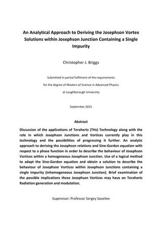
Fig 5.7 – Plot of sine of the phase of a Josephson vortex for different speeds of propagation.
This graph shows the current characteristics with position of the Josephson vortices.
From Fig 5.7, we can see that the maximum superconducting current that is produced by
each type vortex is exactly the same and is independent upon the speed at which the vortex
is moving. The interesting thing to take from the graph is the relationship between the
speed of the vortex and the current as a function of position. Fig 5.7 suggests that as the
speed of the vortex increases closer to the speed of light, the region in which the current
acts gets smaller meaning we only have a supercurrent across a small piece. This plot shows
that a single fluxon can create a superconducting current across the plates which has the
ability to switch from being positive to negative. In reality, we have multiple Josephson
vortices moving through the junction and we should consider the influence of all of them as
and treat it as a whole. We find that we get a constantly oscillating current (AC Josephson
current), which is able to react with the Josephson Plasma to produce Josephson Plasma
-1.5
-1
-0.5
0
0.5
1
1.5
-4 -3 -2 -1 0 1 2 3 4
Current
v=0.1c v=0.9c v=0.99c

46
waves which can be used as a source of Terahertz radiation. This also shows that the overall
net current for our vortex is zero. By plotting the time derivative of the phase against the
time, Fig 5.8, we can determine the voltage across the junction when a Josephson vortex
propagates through the junction. We can see that the vortex produces a voltage across the
two plates and when we consider multiple Josephson vortices moving within the junction,
we see that there is a constantly oscillating voltage across the plates. These two
mechanisms (alternating Josephson current and alternating voltage) are the cause of THz
wave production within a Josephson junction, which makes them highly favourable for use
within Terahertz Technology.
Fig 5.8 – Plot of the time derivative of a single Josephson vortex at the positon where x=0 for
different speeds of propagation. This represents the voltage across the junction.
In order to explain the relationship between the phase and the magnetic field, we should
plot the position derivative of the phase as shown by Fig 5.9.
-14
-12
-10
-8
-6
-4
-2
0
-4 -3 -2 -1 0 1 2 3 4
dϕ/dt
v=0.5 v=0.9 v=0.99

47
Fig 5.9 – Plot of the change in phase of a Josephson vortex as a function of position for
different speeds of propagation.
This is a very important graph as it is able to explain the magnetic field strength within
Josephson junction as a result of the Josephson vortices. From equation (5.11), we know
that the strength of the magnetic field is related to the derivative of the phase with respect
to position by some coefficient which depends upon the distance between the two plates.
By using this relation we can see that the magnetic field strength is greatest when the
Josephson vortices are moving at higher speeds, however the important observation from
this plot is related to the width of the curves. The width of each curve is directly
proportional to the penetration depth of the magnetic field. This means that as the speed of
the Josephson vortex approaches the speed of light, the distance that the magnetic field can
penetrate into the junction reduces. Another interesting observation that can be made from
this plot is that if look at the area under each curve, they are all the same which suggest that
0
2
4
6
8
10
12
14
-4 -3 -2 -1 0 1 2 3 4
dϕ/dx
v=0.1c v=0.9c v=0.99c

48
the magnetic flux passing through is the same regardless of the speed of the Josephson
vortex.
5.5 – Inhomogeneous Sine-Gordon Equation
Now that we have discussed the formation of Josephson vortices within a homogeneous
Josephson junction, we now have a basis to compare the function we will obtain from
looking at an inhomogeneous Josephson junction. The wave function within the junction
plays a huge role in the determination of the electrodynamic properties of a Josephson
junction as is stated by the Josephson relations so the primary goal from here is to be able
to formulate a wave function within an “imperfect” Josephson junction. When we looked at
the perfect and homogenous Josephson junction we made the assumption the junction was
uniform throughout; however in reality the junction may contain some impurities which
prevent the junction being uniform. These impurities can come in many forms such as an
increase in the thickness of the isolating layer at some point or a different type of atom
within the lattice structure of the superconductor at some point. These impurities mean
that we cannot use the perfect case to derive the wave function that propagates within
these junctions.
In order to find the wave function for an inhomogeneous junction we should consider the
simplest case of a Josephson junction with a singular impurity and adapt the Sine-Gordon
equation to compensate for this and then formulate a method of obtaining the solution to
the equation which will give us the wave function for a single impurity Josephson junction.
By using this method to obtain the wave function, we will have devised a method which
should be easily adaptable to accommodate multiple impurities relatively simply.

49
Let us start with a case very similar to that one discussed for the homogeneous, however we
are going to add an impurity at the point where x is zero as shown in Fig 5.10. We are going
to use the idea the waves within the junction can be thought of as a superposition of all the
waves that can propagate within the junction. In order to find the wave function we must
make that assumption that the inhomogeneity within the junction only has an effect on the
wave function over a small distance L.
Fig 5.10 – Basic arrangement of a Josephson junction with an impurity at the point where x is
zero. The presence of the impurity only has an effect on the function over a short distance L
between the positions x = - L/2 and x = L/2.
In order to make the assumption that the wave function is only affected within the small
distance L we must formulate the function that arises as a result of the impurity such that as
the position tends towards positive or negative infinity, the function tends towards zero
which will present us with the generic outline of the wave function stated in equation (5.42).
𝜑 = �
𝜑0 + 𝜑1 𝑓𝑓𝑓 𝑥 ≤ �
𝐿
2
�
𝜑0 𝑓𝑓𝑓 �
𝐿
2
� < 𝑥 (5.42)

50
By making this assumption, we can treat the case when the wave function isn’t affected by
the impurity to have a solution exactly the same to that of the homogeneous Josephson
junction solution as shown in equation (5.43).
𝜑 =
⎩
⎪
⎨
⎪
⎧4 arctan �𝑒
𝑥−𝑣𝑣
√1−𝑣2
� + 𝜑1 𝑓𝑓𝑓 𝑥 ≤ �
𝐿
2
�
4 arctan �𝑒
𝑥−𝑣𝑣
√1−𝑣2
� 𝑓𝑓𝑓 �
𝐿
2
� < 𝑥
(5.43)
Seeing as though we already know part of the solution to the wave function, the process of
finding the overall solution should be much easier. The next problem that we come across is
within the Sine-Gordon equation. Unlike before when we were able to say the plasma
frequency and the Josephson penetration depth were constants, we can no longer do that
when we have an impurity within the junction. The reason for this is that when the wave
meets the impurity the frequency may be altered as a result of reflection and superposition,
meaning that the plasma frequency now has some dependency upon position and the same
for the Josephson penetration depth. In order to solve this problem we must adapt the Sine-
Gordon equation to be used in the affected region to compensate for the additional phase
function and the position dependence of the two “constants.” By making the change to the
two “constants small” we can use a Taylor expansion to derive the new coefficient as shown
in equations (5.44) and (5.45).
𝜆𝐽 = 𝜆𝐽0 + 𝜆𝐽1(𝑥)
𝜔𝐽 = 𝜔𝐽0 + 𝜔𝐽1(𝑥) (5.44)
1
𝜔𝐽
2
=
1
𝜔𝐽
(0)2 −
2𝜔𝐽1(𝑥)
𝜔𝐽0
3
+
3𝜔𝐽1
2(𝑥)
𝜔𝐽0
4
…
(5.45)
As discussed before, the effect that the impurity has on the plasma frequency is relatively
small in comparison to the original plasma frequency such that any terms where the new

51
plasma frequency with position dependence (denoted by ωJ1(x)) that have powers greater
than one are sufficiently small that they can be approximated to be zero. We must also use
a Taylor expansion upon the sine function as illustrated in equation (5.46). Similar to the
plasma frequency adaptions, we are going to ignore terms where the power of the new
phase 𝜑1 is greater than one.
sin(𝜑) = sin(𝜑0 + 𝜑1)
sin(𝜑) ≈ sin(𝜑0) + (cos(𝜑0))𝜑1 − (sin(𝜑0))
𝜑1
2
2 (5.46)
By substituting these new coefficients in place of the original ones within the Sine-Gordon
equation and replacing the original phase with a superposition of the two phases, we obtain
our adapted version of the Sine-Gordon equation for Josephson junctions with a single
impurity as presented by equation (5.47). This equation will be the focus of our attention in
order to devise a function that explains the effect of inhomogeneity upon the phase of
vortices and waves propagating within the junction.
1
𝜔𝐽0
2
�
𝑑2
𝜑0
𝑑𝑡2
+
𝑑2
𝜑1
𝑑𝑡2
� −
2𝜔𝐽1(𝑥)
𝜔𝐽0
3
�
𝑑2
𝜑0
𝑑𝑡2
+
𝑑2
𝜑1
𝑑𝑡2
� + sin(𝜑0) + (cos(𝜑0))𝜑1
= 𝜆𝐽0
2 𝑑2
𝜑0
𝑑𝑥2
+ 𝜆𝐽0
2 𝑑2
𝜑1
𝑑𝑥2
+ 𝜆𝐽1
2
(𝑥)
𝑑2
𝜑0
𝑑𝑥2
+ 𝜆𝐽1
2
(𝑥)
𝑑2
𝜑1
𝑑𝑥2 (5.47)
In order to simplify this equation to one that is solvable, we must make another assumption.
We assume that the new phase function 𝜑1 only changes slowly with both time and
position. This means that although the first differential and second differential with respect
to both time and space will not be equal to zero, the second differential will be very small.
This means that when we combine this with the x dependent coefficients it will be
sufficiently small that we can approximate these terms to be zero, which results in equation
(5.47) being simplified to equation (5.48).

52
1
𝜔𝐽0
2
�
𝑑2
𝜑0
𝑑𝑡2
+
𝑑2
𝜑1
𝑑𝑡2
� −
2𝜔𝐽1(𝑥)
𝜔𝐽0
3
𝑑2
𝜑0
𝑑𝑡2
+ sin(𝜑0) + (cos(𝜑0))𝜑1
= 𝜆𝐽0
2 𝑑2
𝜑1
𝑑𝑥2
+ 𝜆𝐽1
2
(𝑥)
𝑑2
𝜑0
𝑑𝑥2 (5.48)
Due to the fact that we know what 𝜑0 is, we can substitute this in to further simplify the
equation. However considering we have already proven that both sides of the Sine-Gordon
equation are equal for our given Josephson vortex function 𝜑0, we can simply cancel the
terms from the original Sine-Gordon equation as we know that they all cancel out anyway.
This leaves us with equation (5.49).
1
𝜔𝐽0
2
𝑑2
𝜑1
𝑑𝑡2
−
2𝜔𝐽1(𝑥)
𝜔𝐽0
3
𝑑2
𝜑0
𝑑𝑡2
+ (cos(𝜑0))𝜑1 = 𝜆𝐽0
2 𝑑2
𝜑1
𝑑𝑥2
+ 𝜆𝐽1
2 𝑑2
𝜑0
𝑑𝑥2 (5.49)
In order to put this into a solvable format, we must simplify the cosine term by replacing the
phase with our solution from before. Like when we calculated the sine of the solution
before for the homogenous equation, we are going to use the compound angle formula to
simplify the function as shown in equation (5.50).
cos(𝜑0) = cos �4 𝑎𝑎𝑎𝑎𝑎𝑎 �𝑒
𝛼
𝜆 𝐽�� = cos(4𝛽)
cos(4𝛽) = 1 − 8𝑠𝑠𝑠2(𝛽) + 8𝑠𝑠𝑠2
(𝛽)
cos(𝜑0) =
𝜃4
− 6𝜃2
+ 1
𝜃4 + 2𝜃2 + 1 (5.50)
This function works in a similar way to a potential function and allows us to devise a means
of solving the equation using an approximate approach to the problem. If we are to plot the
potential function against position when we take the time to be zero we obtain the plot
shown in Fig 5.11.

53
Fig 5.11 – Plot of the potential function against position when time is taken to be zero. The
plot shape looks very similar to that of the differential of the phase obtained from the
homogeneous Josephson junction.
Now that we have simplified the cosine term, we can substitute it back into the equation in
order to give us the final Sine-Gordon equation as shown in equation (5.51). This equation
will be the focus of the project and we will attempt to solve it using an analytical approach
in order to determine a function which can describe the propagation of Josephson vortices
and plasma waves within a Josephson junction that contains impurities.
𝜃 = 𝑒
𝑥−𝑣𝑣
√1−𝑣2
1
𝜔𝐽0
2
𝑑2
𝜑1
𝑑𝑡2
−
2𝜔𝐽1(𝑥)
𝜔𝐽0
3
𝑑2
𝜑0
𝑑𝑡2
+
𝜃4
− 6𝜃2
+ 1
𝜃4 + 2𝜃2 + 1
𝜑1 = 𝜆𝐽0
2 𝑑2
𝜑1
𝑑𝑥2
+ 𝜆𝐽1
2 𝑑2
𝜑0
𝑑𝑥2 (5.51)
5.6 – Inhomogeneous Wave Solution
5.6.1 – WKB Method
The first proposed method of solving this type of equation was to use a method that can
solve linear differential when the coefficients aren’t constants using an approximation
method. The suggested method to use was the Wentzel-Kramers-Brillouin (WKB)
approximation. This method is commonly used in Quantum Mechanics and is an
approximation which can be applied to second order differential equations in order to

54
estimate a value for the second derivative of a function. The WKB method deals with
equations which are in the form shown in equation (5.52).
𝑑2
𝑦
𝑑𝑑2
+ 𝑘0
2
𝑓(𝑥)𝑦 = 0 (5.52)
This type of equation is usually relatively simple to solve without an approximation method
when the f(x) term is a constant and generates solution in the form of equation (5.53). For
example by considering a wave propagating through a medium with constant dielectric
impedance (i.e. f(x) is the dielectric impedance) with the second order differential equation
similar to that in (5.52), we obtain the solution by using an Ansatz function and calculating
the values of the constants by substituting it into the differential equation. This will
generate a solution similar to that in equation (5.53).
𝑦 = 𝑦(𝑥) = 𝐴𝑒−𝑖𝑘0�𝑓(𝑥)𝑥 (5.53)
This method is very suitable for the cases where we have a constant f(x) term, however in
reality this may not be the case and in such situations the original method for calculating
second order differential equation is invalid and inaccurate. Going back to the example
about the dielectric impedance, it is possible that the impedance of the material can change
the deeper into the medium the wave moves as a result of a change in density or impurities
in the medium. To solve this problem we treat the problem by allowing for f(x) to vary
slowly with respect to x, in order to allow us to make predictions about the second order
derivative. Due to the slower variation within x, we can tell that the first differential won’t
be zero and that the second differential will be sufficiently small that we can approximate it
to be zero. This allows us to make an approximation for the value of the second order
derivative. In order to do this, still using the example of the dielectric impedance, we need
to define the change in phase of the wave as μ and the square root of f(x) by n(x).

55
Substituting these into equation (5.52) using the wave of the form shown in equation (5.53)
with the newly defined variables, we obtain the result shown in equation (5.55).
𝑑𝑑 = 𝑘0 𝑛(𝑥)𝑑𝑑
∆𝜇 = 𝑘0 � 𝑛(𝑥)𝑑𝑑
𝑥
0 (5.54)
𝑑2
𝑦
𝑑𝑑2
+ 𝑘0
2
𝑛2
𝑦 = −𝑘0
2
��
𝑑𝑑
𝑑𝑑
�
2
𝑥2
+ 2𝑛𝑛 �
𝑑𝑑
𝑑𝑑
�� 𝑦 − 𝑖𝑘0 �
𝑑2
𝑛
𝑑𝑑2
𝑥 + 2
𝑑𝑑
𝑑𝑑
� 𝑦
(5.55)
As we have outlined before f(x) varies with position, and therefore n(x) does as well, so the
first differential of n(x) cannot be equal to zero. By substituting our function for change in
phase into our Ansatz (as shown in equation (5.56)), we can place this into our differential
equation in order to give the following equation which we can use to approximate the
second order differential.
𝑦(𝑥) = 𝐴 exp(−𝑖𝑘0∆𝜇𝜇)
𝑦(𝑥) = 𝐴 exp(−𝑖𝑘0 �� 𝑛(𝑥)𝑑𝑑
𝑥
0
� 𝑥
(5.56)
�− �
𝑑𝑑
𝑑𝑑
�
2
+ 𝑖
𝑑2
𝜇
𝑑𝑑2
+ 𝑘0
2
𝑛2(𝑥)� 𝑦(𝑥) = 0
(5.57)
From equation (5.57), we can state that either the square bracket is equal to zero or y(x) is
equal to zero. However for our solution to hold any physical relevance, the square bracket
must equal zero as y(x) being equal to zero would mean that the wave is not propagating. As
a result of making the square bracket equal to zero and using the first approximation that
the second derivative is approximately equal to zero we are able to derive a function that
relates the first derivative of the phase to n(x).

56
�
𝑑𝑑
𝑑𝑑
�
2
≈ 𝑘0
2
𝑛2(𝑥)
𝑑𝑑
𝑑𝑑
≈ ±𝑘0 𝑛(𝑥) (5.58)
Through the use of equation (5.58), we are able to differentiate the equation in order to
obtain an approximate value for the second derivative of the phase which we can substitute
back into the square bracket of equation (5.57). This allows us to acquire a second
approximation for the first derivative, which in turn allows us to calculate the phase and
therefore original wave function.
− �
𝑑𝑑
𝑑𝑑
�
2
+ 𝑖 �±𝑘0
𝑑𝑑
𝑑𝑑
� + 𝑘0
2
𝑛2(𝑥) = 0
𝑑𝑑
𝑑𝑑
≈ ±𝑘0 𝑛 +
𝑖
2𝑛
𝑑𝑑
𝑑𝑑 (5.59)
𝜙(𝑥) = ±𝑘0 � 𝑛(𝑥)𝑑𝑑 +
𝑖
2
ln�𝑛(𝑥)�
𝑥
𝑥0
(5.60)
𝑦±(𝑥) =
𝐴
�𝑛(𝑥)
exp(±𝑖𝑘0 � 𝑛(𝑎)𝑑𝑑)
𝑥
𝑥0 (5.61)
This result differs from other techniques as it compensates for a variation within the
properties of the medium as position changes. As a result we obtain a function which can
better describe the change in phase of a wave function as it moves through the medium and
the impedance or property that resists the movement of the wave changes throughout. This
method is also able to describe the dependence of the amplitude of the wave upon the
properties of the medium. As we would expect, it is possible for the amplitude to decrease
as the wave moves within the medium due to the dissipation of energy.
One of the main changes that we will have to make in order to use this technique for the
case of a Josephson junction with a single impurity comes from the variables within the

57
differential equation. Normally, we would only use the WKB method for cases where the
function only has a dependence upon either position or time however the adapted Sine-
Gordon equation has a dependence upon both. In order to compensate for this, we have to
adapt the method to be applicable to a multi-variable evolution problem (Bracken and Paul,
2006). This method states that we should consider the amplitude and phase to both have a
reliant on time and space as stated in equation (5.62).
𝜑1(𝑥, 𝑡) = 𝐴(𝑥, 𝑡)𝑒 𝑖𝑖(𝑥,𝑡) (5.62)
By using this function as our Ansatz and place it into the differential equation, we are able to
obtain an equation very similar to that we obtain from the WKB method with a single
variable. However in order to do that, we must rearrange the Sine-Gordon equation that we
obtained for the inhomogeneous Josephson junction such that we have all terms that are
derivatives of the original vortices on one side and all the terms that are derivative of the
unknown wave function on the other.
1
𝜔𝐽0
2
𝑑2
𝜑1
𝑑𝑡2
− 𝜆𝐽0
2 𝑑2
𝜑1
𝑑𝑥2
+
𝜃4
− 6𝜃2
+ 1
𝜃4 + 2𝜃2 + 1
𝜑1 =
2𝜔𝐽1(𝑥)
𝜔𝐽0
3
𝑑2
𝜑0
𝑑𝑡2
+ 𝜆𝐽1
2 𝑑2
𝜑0
𝑑𝑥2 (5.63)
The next step to make this equation useable within the WKB method is to introduce a Delta
function to the right hand side such that it follows equation (5.64).
𝛿(𝑥) = �
𝑓(𝑡) 𝑓𝑓𝑓 𝑥 = 0
0 𝑓𝑓𝑓 𝑥 ≠ 0 (5.64)
1
𝜔𝐽0
2
𝑑2
𝜑1
𝑑𝑡2
+ 𝜆𝐽0
2 𝑑2
𝜑1
𝑑𝑥2
+
𝜃4
− 6𝜃2
+ 1
𝜃4 + 2𝜃2 + 1
𝜑1 =
2𝜔𝐽1(𝑥)
𝜔𝐽0
3
𝛿(𝑥)
𝑑2
𝜑0
𝑑𝑡2 (5.65)
Using equation (5.62) and substituting it into (5.65), obtain an equation very similar to that
within the single variable WKB method. This equation is then rearranged such that we have

58
time derivatives on one side and position derivatives on the other as represented in
equation (5.66).
1
𝜔2
�
𝜕2
𝐴
𝜕𝜕2
+ 2𝑖
𝜕𝜕
𝜕𝜕
𝜕𝜕
𝜕𝜕
+ 𝑖𝑖
𝜕𝜕
𝜕𝜕
− 𝐴 �
𝜕𝜕
𝜕𝜕
�
2
� + 𝑓(𝑥)𝐴(𝑥, 𝑡)𝑒 𝑖𝑖(𝑥,𝑡)
= 𝜆2
�
𝜕2
𝐴
𝜕𝜕2
+ 2𝑖
𝜕𝜕
𝜕𝜕
𝜕𝜕
𝜕𝜕
+ 𝑖𝑖
𝜕𝜕
𝜕𝜕
− 𝐴 �
𝜕𝜕
𝜕𝜕
�
2
�
(5.66)
This can then be arranged into two equations: one consisting of the real parts of the
equation (equation (5.67)) and one consisting of the imaginary part of the equation
(equation (5.68)).
1
𝜔2
�
𝜕𝜕
𝜕𝜕
�
2
−
1
𝜔2 𝐴
𝜕2
𝐴
𝜕𝜕2
+
𝜆2
𝐴
𝜕2
𝐴
𝜕𝜕2
− 𝜆2
�
𝜕𝜕
𝜕𝜕
�
2
− 𝑓(𝑥) = 0 (5.67)
2𝑖
𝜔2 𝐴
𝜕𝜕
𝜕𝜕
𝜕𝜕
𝜕𝜕
+
𝑖
𝜔2 𝐴
𝜕𝜕
𝜕𝜕
−
2𝑖𝑖2
𝐴
𝜕𝜕
𝜕𝜕
𝜕𝜕
𝜕𝜕
− 𝑖𝑖2
𝜕𝜕
𝜕𝜕
= 0 (5.68)
This presents us with the basis for solving the problem of a Josephson junction with a single
impurity using the WKB method. It is possible to solve the equation using this method
however it may not prove very effective for this given situation. Due to the complexity of
equations (5.67) and (5.68), it will be very difficult to use the WKB method to solve this
problem as in order to approximate the value for either the second differential with respect
to position or with respect to time we will have to produce an approximation that relates to
the second differential of the other. This means that we will not be able to use the
approximation to calculate the second derivative with respect to the other variable as we
require the two to be separable in order to produce a physically possible solution. Also as a
result of the second derivative for both position and time within the imaginary part of the
solution, we are unable to fully eliminate A in order to allow us to calculate S. This equation
can be used with the use of computer software with high computational time; however it is

59
likely to produce overly complicated functions that aren’t possible to plot. With this in mind,
we are likely to have more success by using an analytical approach based around the wave
equation in order to produce a viable solution.
5.6.2 – General Solution using Wave Equation
In order to determine a function for the wave function as a result of the impurity within the
junction we should consider the case where we take x to be zero in order to give us a
hyperbolic differential equation which we may solve in order to produce a general solution.
This general solution will then allow for us to use boundary conditions as well as initial
constraints in order to produce a particular solution to this equation based around our
problem. The first step in order to do this is to outline a second order differential equation
as shown below.
1
𝜔𝐽0
2
𝜕2
𝜑1
𝜕𝜕2
− 𝜆𝐽0
2 𝜕2
𝜑1
𝜕𝑥2
= 0
(5.69)
This is a hyperbolic second order partial differential equation and is very similar to the
simplest case of the wave equation which is able to describe the motion of all waves. This
equation can be rearranged to produce equation (5.70), in order to make it simpler to find
the general solution of the wave.
𝛼 = 𝜆𝐽0 𝜔𝐽0
�
𝜕
𝜕𝜕
+ 𝛼
𝜕
𝜕𝜕
� �
𝜕
𝜕𝜕
− 𝛼
𝜕
𝜕𝜕
� 𝜑1 = 0 (5.70)
In order to solve this equation, it may be beneficial to change the coordinate system in
order to make this easier to solve for the general solution. We are going to do this in such a
way that the new coordinate system follows the criteria outlined in equation (5.71).

60
𝜑1(𝑥, 𝑡) = 𝜓(𝜉, 𝜂)
𝜉 = 𝑥 + 𝛼𝛼
𝜂 = 𝑥 − 𝛼𝛼 (5.71)
This allows us to rearrange equation (5.70) such that we have a single second order
differential term which is equal to zero. We can then integrate this twice, with respect to
each variable once, which will give us the general solution in terms of the new coordinate
system.
𝜕2
𝜓
𝜕𝜕𝜕𝜕
= 0
𝜓(𝜉, 𝜂) = �
𝜕2
𝜓
𝜕𝜕𝜕𝜕
𝑑𝑑𝑑𝑑 = 𝐹(𝜉) + 𝐺(𝜂)
(5.72)
By converting this back into our original coordinate system, we obtain the general solution
in terms of position and time.
𝜑(𝑥, 𝑡) = 𝑓(𝑥 + 𝛼𝛼) + 𝑔(𝑥 − 𝛼𝛼) (5.73)
This is a very common general solution for wave based equations and each function
represents a wave travelling in the opposite direction to each other. There is another
method that can be used to derive this equation which can be used to check that the
general solution obtained is correct. By rearranging equation (5.69) such that we have the
form shown in equation (5.74), we can treat the wave as some function of p and
differentiate each term twice with respect to p.
1
𝜔𝐽0
2 𝜆𝐽0
2
𝜕2
𝜑1
𝜕𝜕2
−
𝜕2
𝜑1
𝜕𝑥2
= 0
(5.74)

61
𝜑1(𝑥, 𝑡) = 𝑓(𝑝)
𝜕2
𝜑
𝜕𝜕2
= 𝑎2
𝑑2
𝑓
𝑑𝑑2
𝜕2
𝜑
𝜕𝜕2
= 𝑏2
𝑑2
𝑓
𝑑𝑑2 (5.75)
By introducing a new constant, as shown below in equation (5.76), and by dividing through
by the derivative, we can remove the derivative from the equation so we can find a function
for the new variable. We now get a function which tells us the dependence of the general
solution upon time and this solution yields the same solution as calculated using other
methods.
𝑏
𝑎
= 𝜀
𝑎2
𝑑2
𝑓
𝑑𝑑2
−
1
𝜔𝐽0
2 𝜆𝐽0
2 𝑏2
𝑑2
𝑓
𝑑𝑑2
= 0
1 −
1
𝜔𝐽0
2 𝜆𝐽0
2 𝜀2
= 0
𝜀 = ±𝜔𝐽0 𝜆𝐽0
∴ 𝜑1(𝑥, 𝑡) = 𝑓�𝑥 + 𝜆𝐽0 𝜔𝐽0 𝑡� + 𝑔(𝑥 − 𝜆𝐽0 𝜔𝐽0 𝑡) (5.76)
5.6.3 – Boundary Conditions
In order to solve this type of equation for a particular problem we need to outline some of
the initial conditions that the solution must possess as well as some of the constraints the
wave has to follow. The boundary condition which we are going to apply, relates to the
solution when the position is zero. The point where position is equal to zero relates to the
position at which the impurity is situated within the junction. As a result of this point we
would expect the first derivative of the phase function would be equal to some function of

Dissertation

Recommended

Recommended

More Related Content

Similar to Dissertation

Similar to Dissertation (20)

Dissertation