1. The problem of mapping mortality rate:
geocoding complexity
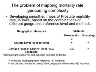
• Developing smoothed maps of Prostate mortality
rate, in Iowa, based on the combinations of
different geographic reference level and methods.
Geographic references Methods
Downscalin
g
Upscaling
County Level (99 locations)
* *
City and “rest of county” level (1053
Locations)
N/A
*
•Computing the observed and expected numbers of deaths
 for county level geographic reference (99 locations)
 for city and “the rest of county” level geographic reference (1053 locations)

2. Downscaling and Upscaling methods
Downscaling
Upscaling
Inverse Distance Weight
Kernel Filter Method
Spatial Model
Measurement
Model

3. Mortality Data
Individual prostate cancer mortality data (year 1999-2003)
associated with city codes and county codes in Iowa
was provided by Iowa Department of Public Health. An
made up example shows as following:
Date_Death sex Age Date_Birth County_Resid City_Resid
1/13/2010 M 83 12/20/1900 029 BUR
1/14/2010 M 67 12/21/1900 029 SPI
1/15/2010 M 82 12/22/1900 030 SPI
1/16/2010 M 71 12/24/1900 041 KEO
1/16/2010 M 74 12/23/1900 041 XXX
• Some death records are outside of city limits but within the
corresponding county
•Some cities across different counties

4. Figure 1: Example of cities crossing different counties
Male Population
Area Number
WEST
BRANCH 1039
Cedar (Part) 997
Johnson
(Part) 42

5. Compute the observed and expected numbers of deaths
for county level, 99 locations
• Creating the geographic location
files
– County centroid file
• Aggregating mortality records
based on corresponding county
code combination
• Assigning the observed aggregated mortality records of
rest counties to the county centroid file
• The expected number of deaths was calculated by
indirectly standardization for age for these counties
centroids
•Calculating statewide standard mortality rate for different age categories
•Obtaining population of each age category for county1
1: available from State Date Center of Iowa http://data.iowadatacenter.org/browse/places.html#PopulationbyCounty

6. • Multiplying the population of each age category with
corresponding statewide standard mortality rate to get
expected number of deaths for each age category in
each county
• Summing all the expected numbers of deaths in each
age category together to obtain the total expected
number of deaths for each county
• Assigning those values to corresponding county
centroids
Compute the observed and expected numbers of deaths
for county level, 99 locations (continued)

7. Assigning observed mortality records to
city and “rest of county” locations
• Creating another geographic
location file
– City point location file (only one
point location for boundary
crossed city) based on populated
places point file2
• Aggregating mortality records
based on corresponding
unique city/county code
combination
2: available from NRGIS library http://www.igsb.uiowa.edu/nrgislibx/gishome.htm
• Assigning the observed aggregated mortality records of
cities to the city point location file
• Assigning the observed aggregated mortality records of
rest counties to the county centroid file

8. Process to compute expected numbers of
deaths for city and “rest of county” locations
• The expected number of deaths was
calculated after the adjustment of age for
these cities and counties centriods
– Statewide standard mortality rate for different
age categories
– Population of each age category for cities3
– Population of each age category for the rest
of county
3: available from State Date Center of Iowa http://data.iowadatacenter.org/browse/places.html#PopulationbyCounty

9. • Compute the population of each age category for the rest of county
County City M0_39 M40_44 … M85A
Cedar 111546 14741 … 1370
City A (fully located within County) Pop_A_1 Pop_A_2 … Pop_A_11
City B (fully located within County) Pop_B_1 Pop_B_2 … Pop_B_11
…
…
…
…
…
West Branch
(Partly located in County) Partial_Pop_1 Partial_Pop_2 … Partial_Pop_11
Pop of each age category for
the rest of Pork county Result_1 Result_2 … Result_11
County City M0_39 M40_44 … M85A
Johnson 11470 1618 … 203
City A (fully located within County) Pop_A_1 Pop_A_2 … Pop_A_11
City B (fully located within County) Pop_B_1 Pop_B_2 … Pop_B_11
…
…
…
…
…
West Branch
(Partly located in County) Partial_Pop_1 Partial_Pop_2 … Partial_Pop_11
Pop of each age category for
the rest of Pork county Result_1 Result_2 … Result_11
Process to compute expected numbers of deaths
for city and “rest of county” locations (continued)

10. • Multiplying the population of each age category with
corresponding statewide standard mortality rate to get
expected number of deaths for each age category
• Summing all the expected numbers of deaths in each
age category together to obtain the total expected
number of deaths for each city and rest of county
• Assigning those values to corresponding city and county
centroids
• Combining city point file and county centroid file together.
We obtained a point file which contains 1053 point
locations and corresponding observed and expected
numbers of deaths.
Process to compute expected numbers of deaths
for city and “rest of county” locations (continued)

11. Create smoothed Prostate mortality
map
Figure 2: Indirect age standardized prostate cancer mortality in Iowa (1999-2003)
using Inverse Distance Weight (IDW) and county centroids for geocodes (99 areas):

12. Create smoothed Prostate mortality
map (continued)
Figure 3: Indirect age standardized prostate cancer mortality in Iowa (1999-2003)
using a fixed distance filters and county centroids for geocodes (99 areas):
a – 30 mile fixed distance filter b – 40 mile fixed distance filter
Correlation coefficient=0.65

13. Create smoothed Prostate mortality
map (continued)
Figure 4: Indirect age standardized prostate cancer mortality in Iowa (1999-2003)
using a fixed distance filters and city and “rest of county” geocodes (1053 areas)
a – 30 mile fixed distance filter b – 40 mile fixed distance filter
Correlation coefficient=0.73