1. Introduction
• TEAL programs have been in use by colleges since the late 1990’s.
• Main goal is to create a classroom that merges lectures,
simulations, and hands-on demonstrations
• In the Fall of 2013 MSU fully introduced a TEAL designed classroom
and a modified (randomization based) curriculum as an alternative to
the traditional lecture style course for STAT 216.
• Randomization curriculum started with CATALST materials
(www.tc.umn.edu/~catalst/) and has evolved over time while some
sections retained consensus (traditional, formula-based) materials.
Randomization vs. Consensus Curricula in Introductory Statistics
Charlie Carpenter, Dr. Mark Greenwood, Dr. Jennifer Green, Dr. Jim Robison-Cox
Department of Mathematical Sciences, Montana State University
Data Visualization
• Figure 3 suggests that relationships
are relatively linear between 216
and 217 GPA points and very similar
for all non-Deveaux 216 students.
• DeVeaux mean possibly higher for
lower 216 GPA with possible
decrease in slope for higher 216
GPA.
• Suggests possible interaction
between 216 GPA and Curricula
or at least different intercepts
• Figure 1 shows skewed distributions for
each curriculum caused by the censoring
of students performance based on a
maximum of 4.0=A.
• Much larger sample size for DeVeaux
than others.
• All means appear to be comparable
among curricula with CAT3 and DeVeaux
having the two highest.
• CAT3 is most recent version of 216
curriculum in our data set.
• Had highest cumulative GPA and least
time between taking 216 and 217.
Testing for Curriculum Differences
• Figure 2 shows strong, positive linear
relationship between previous GPA and
STAT 217 performance.
• No visual evidence of differing slopes
among curricula.
• DeVeaux group possibly has slightly
higher mean.
Methods
• Censored response regression model (Yee, 2015)
• Tobit regression models estimate unobserved means for censored observations
• Generalization of original Tobit Regression (Tobin, 1958)
• For right censoring at a grade of A=4.0:
𝑦𝑖
∗
= 𝛽𝑥𝑖
′
+ 𝜀𝑖
𝑦𝑖 =
𝑦𝑖
∗
𝑖𝑓 𝑦𝑖
∗
< 4
4 𝑖𝑓 𝑦𝑖
∗
≥ 4
• More appropriate modeling structure for a censored response than a regular linear
model.
• Gives us the potential to detect and measure relationships that are dampened
out by censored observations.
• Residuals with regular linear model impacted by censoring
• When responses are observed below the upper censoring limit (A), then the model
is a regular normal likelihood linear model.
• 217 GPA appears to be censored in Figures 1, 2, and 3.
• Students can not earn more than 4 GPA points in 217.
• Distributions appear normal around the mean (or mean for value of predictors)
except many observations accumulating at this upper bound.
• Full model for 217 grade based on cumulative GPA, 216 Grade, Curriculum (5 levels)
and interaction between 216 grade and curriculum:
𝐺𝑃𝐴217 ~ 𝑃𝑅𝐸𝑉𝐺𝑃𝐴 + 𝐺𝑃𝐴216 + 𝐶𝑢𝑟𝑟𝑖𝑐 + 𝐺𝑃𝐴 216: 𝐶𝑢𝑟𝑟𝑖𝑐
• No evidence of an interaction between 216 GPA and curriculum
• 𝜒4
2
= 2.684, p-value = 0.612
• Removing interaction from model.
• Final model for 217 grades:
𝐺𝑃𝐴217 ~ 𝑃𝑅𝐸𝑉𝐺𝑃𝐴 + 𝐺𝑃𝐴 216 + 𝐶𝑢𝑟𝑟𝑖𝑐
• Marginal evidence of a curriculum influence on mean 217 GPA after controlling for
previous GPA and STAT 216 GPA
• 𝜒4
2
= 10.053, p-value = 0.0395
• Strong evidence of a relationship between 216 GPA and the mean 217 GPA after
controlling for previous GPA and curriculum.
• 𝜒1
2
= 28.995, p-value < 0.0001
Research Question
• How do students from different STAT 216 curricula perform in STAT
217?
• Specifically, have the curricula changes influenced grades earned
or WDF rates in STAT 217?
• Does the grade in 216 matter, and does its relationship with 217
performance depend on the curriculum?
Data
• Data were collected from 559 MSU students who took STAT 217
ranging from spring of 2013 to fall of 2015.
• Variables of interest:
• STAT 217 performance
• STAT 216 performance
• STAT 216 Curriculum
• Cumulative GPA before taking STAT 217 (previous GPA)
• Performance in a class was measured as GPA points earned.
• Students must have “passed” STAT 216 to be included in this
data set
• Some mistakenly take 217 without a passing grade in 216.
• Only students that had a recorded grade in STAT 216 and in 217
from MSU were considered in this analysis
• Students that “met” 216 requirement in another way were not
considered.
• Students that chose a W did not obtain a “grade” and were only
considered in WDF assessments not presented here.
Curricula Dates Description
Number of
217 Students
DeVeaux
1990 -
Summer 2014
Built around Stats: Data and
Models, Third Edition, by
DeVeaux, Velleman, and Bock.
316
CATALST
Fall 2012 –
Summer 2013
Curriculum as written by the
CATALST authors and used
Tinkerplots software.
36
CAT2
Fall 2013 –
Summer 2014
Shortened Unit 1 and heavily
modified Unit 3 to better fit
Stat 217. Dropped Tinkerplots
in favor of R-Shiny web apps
which we built.
91
CAT3 Fall 2014
Further modifications became
our own course pack using few
of the CATALST activities.
28
Lock
Spring 2014 –
Spring 2015
Lectures were based on Stats:
Unlocking the Power of Data,
Third Edition, by Lock et al.
88
Figure 1. Beanplots of 217 GPAs by 216 curriculum
type
Figure 2. Previous GPA vs 217 GPA with Lowess
smoothers for each curriculum.
Figure 3. 216 GPA vs 217 GPA with Lowess
smoothers for each curriculum.
Coefficient
(DeVeaux as reference level)
Estimate SE Z-Score P-value
216 GPA 0.40 0.0738 5.385 <0.0001
Previous GPA 1.19 0.0992 12.002 <0.0001
CATALST -0.25 0.1449 -1.695 0.0901
CAT2 -0.21 0.0997 -2.082 0.0373
CAT3 -0.37 0.1659 -2.209 0.0272
Locks -0.15 0.1000 -1.494 0.1352
• For every one GPA point earned in 216 the mean 217 GPA is estimated to increase
by 0.4 points (95% CI: 0.25 to 0.54).
• For every one cumulative GPA point the mean 217 GPA is estimated to increase by
1.19 points (95% CI: 0.996 to 1.384)
• DeVeaux has the highest estimated mean 217 GPA after controlling for 216 and
previous GPA.
• CAT3 had the highest mean performance in STAT 217, but after controlling for 216
grade and previous GPA it has the lowest estimated mean performance (-0.37
points lower than Deveaux, 95% CI: -0.692 to -0.041).
crPlots with Tobit Estimates
Conclusions
Research supported by the Montana State University Undergraduate Scholars
Program (Fall 2015-Spring 2016)
• Beanplots (Kampstra, 2008) used to visually compare the distributions of
217 GPAs among the different 216 curricula.
• ggplot2 (Wickham 2009) used with LOWESS smoothers to visually
assess the relationship between 217 GPA and previous GPA, and the
relationship between 217 GPA and 216 GPA by curriculum type.
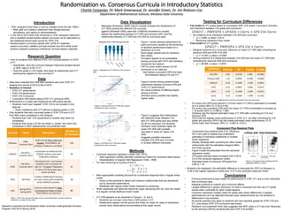
Figure 4. Component plus residuals plots for
quantitative effects in model.
• Component plus residual plots (Fox, Weisburg
2011) are used to assess and understand
estimates of individual coefficients in multiple
linear regression.
• Display residuals after correcting for other model
components with the estimated marginal effect
from least squares.
• Figure 4 adds the estimates from the censored
regression model.
• 216 grade estimate slope increases from 0.29 to
0.4 in the censored regression model.
• Estimated slope for previous GPA goes from
0.96 to 1.19.
• Previous performance does matter for performance in STAT 217 and is more influential
than curriculum type.
• Marginal evidence to support any curriculum effects.
• Largest difference in groups (Deveaux vs Cat3) is reversed from the raw 217 grade
results when controlled for other model aspects.
• Censored regression models useful for grade data where differences in highest
performances can’t be detected because class measurements are not sensitive to
differences in top students.
• All results reported only apply to students who had reported grades for STAT 216 and
217, and whose STAT 216 curriculum was known.
• Research (not presented here) also suggests that WDF rates in 217 are only influenced
by the previous GPA for students that took STAT 216 at MSU.
• Similarly (not displayed), the estimated difference in intercepts for CAT3 vs Deveaux is
-0.06 in the regular regression model and -0.37 in the censored response model.
Component Plus Residual Plots
Table 1: STAT 216 curricula with dates of use, a brief description, and the number of
students in our data set from each.
Table 2: Coefficients and summary information from the final model