1. Stat 154: Text Mining Final Write-Up
Hugo Cortez
Jane Liang
Hiroto Udagawa
Benjamin LeRoy
Monday, May 11, 2015
1. Description
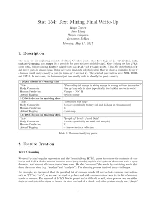
The data we are exploring consists of Stack Overflow posts that have tags of r, statistics, math,
machine-learning, and numpy (it is possible for posts to have multiple tags). Our training set has 27425
posts total, divided among 13268 r tagged posts and 14157 not r tagged posts. Thus, the distribution of r
and not r posts is almost equal. Below are three randomly selected entries that we show as examples to see if
a human could easily classify a post (in terms of r and not r). The selected post indices were 7282, 10206,
and 15710. In each case, the human subject was readily able to classify the post correctly.
7282th datum in training data
Title: "Converting int arrays to string arrays in numpy without truncation"
Body Comments: Has python code in data (specifically has In/Out entries in code)
Human Prediction: Numpy - "Not" R
Actual Tagging: python numpy
10206th datum in training data
Title: "corelation heat map"
Body Comments: R code (specifically library call and looking at visualization)
Human Prediction: R
Actual Tagging: r heatmap
15710th datum in training data
Title: "Length of Trend - Panel Data"
Body Comments: R code (specifically set.seed, and sample)
Human Prediction: R
Actual Tagging: r time-series data.table zoo
Table 1: Humans classifying posts.
2. Feature Creation
Text Cleaning
We used Python’s regular expressions and the BeautifulSoup HTML parser to remove the contents of code
blocks and LaTeX blocks; remove common words (stop words); replace non-alphabet characters with a space
character; and convert all characters to lower case. We also “stemmed” the words by combining words that
share the same stem (e.g. “analyze” and “analysis”). The cleaning process involved many challenges.
For example, we discovered that the provided list of common words did not include common contractions
such as “I’ll” or “can’t”, so we saw the need to go back and add common contractions to the list of common
words to remove. The removal of LaTeX blocks proved to be difficult as well, since posters can use either
single or multiple dollar signs to denote the start and end of a chunk, and other posters simply use “begin”
1

2. and “end”. In addition to matching all of these cases, we needed to modify our regular expressions for LaTeX
blocks in order to avoid matching cases in which people simply used a dollar sign to denote a dollar sign or
something unrelated to LaTeX blocks.
Dictionary of Word Counts
We then derived a dictionary of words and the total number of their appearances throughout the whole data
set. There were 24109 words in total (after filtering out common words and contractions and stemming words
with common stems). Below are some examples of words and the counts of their total number of appearances.
As you can see, the most common word was “use”, and other common words include single-letter words
like “r”, “m”, “s”, and “t”. Many rare and unhelpful words such as “aaaaaaaaajq” appeared a few times
throughout the entire data set and should probably be removed.
Table 2: Dictionary: Top 10 Most Frequent Words.
Word Count
use 23369
r 19600
data 17110
function. 12773
m 12232
valu 11589
s 10959
t 10903
want 10006
tri 9746
Table 3: Dictionary: First 10 in Alphabetial Order.
Word Count
a 812
aa 62
aaa 6
aaaa 2
aaaaaa 2
aaaaaaaaajq 2
aaaaab 2
aaaabbbbaaaabaaaa 2
aaaac 2
aaaaq 2
Word Feature Matrix
Our word feature matrix filters out the aforementioned stop words (both the common words and common
contractions) and rare words (words that do not appear more than 10 times throughout the whole data set).
We merged the title and body words and output a frequency matrix. The original number of word features
after initial cleaning was 24109, but after excluding rare words (those that did not appear more than 10
times), it was 5195. Thus, the word feature matrix was 27425 rows by 5195 columns. We also created a
target vector of having tag r versus not having tag r.
2

3. A major programming challenge was adapting the code used to generate the word feature matrix in order to
avoid memory errors. We used several techniques, such as allocating memory for a sparse matrix of zeros
prior to filling the matrix with counts. Revised versions of our code also minimized the usage of loops and
other inefficient programming methods.
3. Unsupervised Feature Filtering
We approached unsupervised feature selection in two ways. Both took into account variance of the word feature
variables themselves rather than simply creating minimum and maximum thresholds for word appearance.
Definitions of Elements
The word matrix is a very sparse matrix, so there were a couple of ways we looked at the features.
• The first was looking at each feature’s binary variance. To create the “binary” variance we first looked
at each post and saw if the particular word feature appeared once or more in the post. If it did, we
recorded the post as a 1; if it didn’t we recorded it as a 0. After doing this, we took the variance of the
features 1 and 0 entries.
• The second way was looking at each word feature’s count variance. To create the “count” variance
we first looked at each post and counted the number of times the feature appeared in each post and
recorded that integer. Then we took the variance of the features’ count integer values.
Original Cut (Binary Variance)
First, in order to reduce the feature space quickly, we started with the recommended first cut of “rare” word
features that appeared 10 times or fewer throughout the data set. This is very justifiable, not just because
only appearing 10 times is a very small number compared to the total sample size of 27425, but also because
the binary variance of an element that appears in 10 or fewer posts is 10 · ( 1
n − 1
n2 ). In our case, that’s
3.6461752 ·10−4
(n=27425).
Focused Cut (Count Variance)
Since the previous lower bound was quite low, we decided to look at count variance. With previous knowledge
of the time it takes for classification methods in R to process big groups of data, we hoped to get the number
of features to a more reasonable size (the previous rough cut reduced the feature space from 24109 to 5195,
which is still quite a lot of features). We ordered the count variance of these remaining 5195 and looked at
the minimum variance if we only kept a certain number of features. Below is a table of our results:
Table 4: Features kept and variance cutoffs.
Number of Features Kept Proportion Kept (of 5196) Actual Variance Cutoff
1000 0.1924557 0.0183133
900 0.1732102 0.0212428
800 0.1539646 0.0253277
700 0.1347190 0.0311935
600 0.1154734 0.0383534
500 0.0962279 0.0495617
3

4. We noticed that a minimum variance associated with the 500 mark was really close to 0.05 (a small amount
of variance even in sparse data), and we decided our future cutoff would be to include features with count
variance greater than 0.05. With this cutoff in place we kept 501 features for our final word feature matrix.
Below are histograms of the number of times word features appeared in the text before and after we imposed
the 0.05 variance cutoff. As you can see, both histograms are heavily right-skewed. However, the histogram
of the original 5195 words (after the initial cut of those appearing 10 times or fewer) is so skew that it
is barely interpretable. The vast majority of the word features (over 4000) appear very few times. The
histogram of our final word features depicts considerable spread and variation among the words’ appearances.
5195 Word Features
Number of Appearances
Frequency
0 10000 20000
020004000
Final Word Features
Number of Appearances
Frequency
0 10000 200000204060
Final Comments
We think it should be noted that the first basic cut could have been eliminated as part of the second cut, but
we wanted to explain how we approached the problem. Another comment is that we also explored cutting a
similar number of features using the binary variance, but we found a significant difference in the features cut,
and looking at word counts seemed to make more sense. We did observe two outliers in variance (due to
posts having code in the text area, but the benefits still outweighed the costs).
4. Power Feature Extraction
Most of the following power features cannot be directly captured by the word frequency matrix generated in
Part 3 alone. In particular, the word features only focus on the text in the combined title and body of each
post. In general, this was the motivation for adding these power features (to catch what a human eye can
see, but the frequency text analysis cannot). To extract the following power features, we had to do some
additional processing in Python of the raw data using regular expressions and the BeautifulSoup HTML
parser.
A. Counting Number of Blocks
1. nCode: Number of code blocks, marked by <code> HTML tags.
This can help reflect if the question is about code (and counting the number of code blocks can possibly
distinguish between different types of coding questions as well numpy vs r).
2. nLatex_body: Number of LaTeX blocks in body, marked by any number of dollar signs ($) or begin
or end.
4

5. This can help reflect if the question is more theoretical (and counting the number of LaTeX blocks can
possibly distinguish between different types of theoretical and non-theoretical questions as well).
3. nLatex_title: Number of LaTeX blocks in title, marked by any number of dollar signs ($) or begin
or end.
Similar to the nLatex_body rational, we’d expect coding questions (about r, numpy, etc) to have
fewer LaTeX blocks in the title than theoretical questions (more statistics or math related).
B. Counting Number of Elements/Words in Blocks
4. nWords_title: Number of words in title text.
Longer titles might suggest harder-to-explain concepts that would fall into specific categories.
5. nWords_body: Number of words in body text.
A longer body text might suggests harder-to-explain concepts that would fall into specific categories.
6. nWords_code: Number of words in code block (split on blanks).
A longer code block would usually be related to either more complicated code or more multi-parameter
functions in the code (like plot in r).
C. Counting Number of Characters in Blocks
These all have goals similar to those of the power features that count the number of words in the respective
blocks, but may offer additional insights.
7. nChar_title: Number of characters in title text.
8. nChar_body: Number of characters in body text.
9. nChar_latex: Number of characters in body LaTeX blocks.
10. nChar_code: Number of characters in code blocks.
D. Looking for Specific References in Body Text
11. isLink: Binary presence of a link in the body.
Links for websites may generally be associated with “super confusing” things that might gravitate
towards certain classes.
12. isC_body: Binary presence of C references in body text.
We generally cannot detect “C++” and “C#” references after cleaning the text and removing
punctuation, but these program references would definitely encourage some classifications rather than
others (specifically non-r and numpy classifications).
13. isMatlab_body: Binary presence of Matlab references in body text.
We think that this might be redundant with the corresponding variable in the word frequency feature
matrix, but this binary variable would capture the presence of matlab. (Plus in random forest models
it doesn’t really hurt to have very correlated features.) We want to know when certain coding languages
are discussed, since it can indicate certain types of questions.
14. isPython_body: Binary presence of Python references in body text.
We think that this might be redundant with the corresponding variable in the word frequency feature
matrix, but this binary variable would capture the presence of python. (Plus in random forest models
it doesn’t really hurt to have very correlated features.) We want to know when certain coding languages
are discussed, since it can indicate certain types of questions.
E. Looking for Specific References in the Code
The names and descriptions of the following are pretty self-explanatory. We grouped some common words
and code identifiers for certain types of programming languages or processes to try to classify what type of
5

6. code/problems are being addressed in the code blocks.
15. isPyCode: Binary presence of Python code references.
References were: “def”, “import”, “>>>”, “in [”, “out[”.
16. isRCode: Binary presence of R code references.
References were: “<-”, “library”, “set.seed”, “read.csv”.
17. isRVis: Binary presence of R code visualization references.
References were: “heatmap”, “ggplot”.
18. isRBrace: Binary presence of curly braces {} as proxy for R code.
19. isMLCode: Binary presence of machine learning code references (R-style).
References were: “svm”, “cv”, “knn”, “randomforest”, “glm”.
20. isMLKeywords: Binary presence of machine learning code keywords.
References were: “tree”, “ensemble”, “bagging”, “boosting”, “rf”, “forest”, “knn”, “neural networks”,
“logistic”, “perceptron”, “support vector machine”, “svm”, “cluster”.
F. Looking for Key Words in Title Text
Since we combined the title and body text together to make the word feature matrix, these power features
can help emphasize the existence of certain words in the title.
21. isR_title: Binary presence of r in title
22. isNumpy_title: Binary presence of numpy or python in title
23. isML_title: Binary presence of machine learning/machine-learning
24. isStat_title: Binary presence of stats/statistics in title
25. isMath_title: Binary presence of math/maths/mathematics in title
We then stored these 25 power features as our power feature matrix.
5. Word and Power Feature Combination
We created a combined feature matrix with dimensions 27425 × 526 (501 word features and 25 power
features).
6. Classification on the Filtered Word Feature Matrix
Here, we classified posts as r and not r using random forest models. In order to save computation time,
we used a subset of 5000 observations from the original training set of 27425 observations when running
cross-validation to tune the mtry parameter (the number of features randomly sampled as candidates at each
split). We used three different feature matrices to build three separate random forest models.
• The first was the word feature matrix, which includes the frequencies of 501 features (words) that we
deemed most important through the unsupervised method in Part 3.
• The second was the 25 power features that we created in Part 4 by looking at additional aspects such
as total word counts and embedded code.
• Lastly, we looked at the combined word and power feature matrix.
6

7. 10-Fold Cross-Validaton — Word Matrix
For the word feature matrix, we ran 10-fold cross-validation in order to find the optimal mtry value. We
checked a range of twelve mtry values ranging from 1 to 500 (a range chosen to reflect the size of our feature
space), and used 10 trees. The plot of the errors and mtry values is shown below.
Based on the plot, an mtry value of 41 created the minimum error rate.
0 50 100 150
0.100.150.200.25
Word Matrix Cross Validation
mtry
ErrorRate
10-Fold Cross-Validaton — Power Matrix
For the power feature matrix, we again ran 10-fold cross-validation to find the optimal mtry value. This time,
we checked a 10 values ranging from 1 to 10, since there were only 25 total power features, and again used
10 trees. The plot of the errors and mtry values is shown below.
Based on the plot, an mtry value of 4 was optimal for the power feature matrix.
7

8. 2 4 6 8 10
0.140.180.22
Power Matrix Cross Validation
mtry
ErrorRate
10-Fold Cross Validaton — Combined Matrix
Finally for the combined word and power feature matrix, we again ran 10-fold cross-validation to optimize
mtry. We checked the same grid of twelve values ranging from 1 to 500 as with the word feature matrix,
since the combined feature space had similar dimensions, and used 10 trees. The plot of the errors and mtry
values is shown below.
Based on the plot, an mtry value of 31 was optimal for the combined word and power feature matrix.
0 50 100 150
0.050.100.150.20
Combined Matrix Cross Validation
mtry
ErrorRate
8

9. ROC Curve
Next, we used our optimal mtry values to rerun the classification models for each of the three feature matrices
using the entire training set of 27425 observations. The three ROC curves are shown below, with predictions
obtained by running 10-fold cross validation on the entire training set and using a threshold of 0.5 for
classification.
As expected, the combined matrix produced the best ROC curve, hugging the upper left corner the most
closely and resulting in the highest AUC. Of the three, it had the largest feature space and was in fact made
up of the other two. The word matrix generated the second best ROC curve and appeared to do almost as
well as combined, and the power features alone performed the poorest.
Word Matrix ROC Curve
False positive rate
Truepositiverate
0.0 0.2 0.4 0.6 0.8 1.0
0.00.20.40.60.81.0
Power Matrix ROC Curve
False positive rate
Truepositiverate
0.0 0.2 0.4 0.6 0.8 1.0
0.00.20.40.60.81.0
Combined Matrix ROC Curve
False positive rate
Truepositiverate
0.0 0.2 0.4 0.6 0.8 1.0
0.00.20.40.60.81.0
Table 5: AUC for ROC Curves
AUC
Word 0.9867939
Power 0.9425940
Combined 0.9921379
PPV/NPV Analysis
1st Visualization of PPV vs NPV
In the following charts, we looked at the relationship of PPV against NPV at various thresholds, as with the
ROC curves in the previous section. We found this visualization to be difficult to interpret, although the
performance suggested by the area under the curves is consistent with our conclusions based on the ROC
curves.
9

10. Word Matrix
PPV vs NPV
Negative predictive value
Positivepredictivevalue
0.75 0.85 0.95
0.700.800.901.00
Power Matrix
PPV vs NPV
Negative predictive valuePositivepredictivevalue
0.65 0.75 0.85
0.650.750.850.95
Combined Matrix
PPV vs NPV
Negative predictive value
Positivepredictivevalue
0.75 0.85 0.95
0.700.800.901.00
2nd Visualization of PPV vs NPV
In this visualization we fixed the mtry value in RF as
√
number of features for each of the classification
models, and varied the threshold value.
Word Matrix
PPV and NPV
Threshold
PredictiveValue
0.0 0.2 0.4 0.6 0.8 1.0
0.00.20.40.60.81.0
0.0 0.2 0.4 0.6 0.8 1.0
0.00.20.40.60.81.0
Threshold=.52
−
−
PPV
NPV
Power Matrix
PPV and NPV
Threshold
PredictiveValue
0.0 0.2 0.4 0.6 0.8 1.0
0.00.20.40.60.81.0
0.0 0.2 0.4 0.6 0.8 1.0
0.00.20.40.60.81.0
Threshold=.49
−
−
PPV
NPV
Combined Matrix
PPV and NPV
Threshold
PredictiveValue
0.0 0.2 0.4 0.6 0.8 1.0
0.00.20.40.60.81.0
0.0 0.2 0.4 0.6 0.8 1.0
0.00.20.40.60.81.0 Threshold=.53
−
−
PPV
NPV
The threshold at which the PPV curve crosses the NPV curve is around 0.5 for all three models. This is good
because a threshold of 0.5 is generally used by default for classification based on predicted probabilities, even
without exploring the effect of the threshold on the PPV and NPV values. The threshold at which PPV and
NPV intersect is often used because we see optimal rates coming from both metrics, whereas extreme values
of the threshold can lead to one value being high and one value being low. Depending on the goals of one’s
analysis, optimizing one of the two metrics may be more important and thus suggest a different threshold.
3rd Visualization of PPV and NPV
In this visualization, we looked at the plots of PPV and NPV based on changing the mtry values (number of
features available for each branch of the trees generated in the random forest model). Shown below are also
tables of PPV and NPV values depending upon the value of mtry.
10

11. 0 100 300 500
0.00.20.40.60.81.0
Word Matrix
PPV and NPV
mtry
PredictiveValue
PPV
NPV
2 4 6 8 10
0.00.20.40.60.81.0
Power Matrix
PPV and NPV
mtryPredictiveValue
PPV
NPV
0 50 100 150 200
0.00.20.40.60.81.0
Combined Matrix
PPV and NPV
mtry
PredictiveValue
PPV
NPV
Table 6: Word Matrix
1 11 21 31 41 51 61 100 125 150 175 500
PPV 0.7576 0.8938 0.9091 0.9211 0.9218 0.9200 0.9188 0.9214 0.9218 0.9262 0.9266 0.9243
NPV 0.7764 0.9302 0.9393 0.9346 0.9290 0.9307 0.9302 0.9255 0.9214 0.9221 0.9259 0.9185
Table 7: Power Matrix
1 2 3 4 5 6 7 8 9 10
PPV 0.7316 0.7911 0.8342 0.8440 0.8544 0.8484 0.8570 0.8504 0.8462 0.8507
NPV 0.8220 0.8602 0.8697 0.8734 0.8719 0.8586 0.8649 0.8602 0.8598 0.8653
Table 8: Combined Matrix
1 11 21 31 41 51 61 100 125 150 175 500
PPV 0.7968 0.9114 0.9307 0.9363 0.9333 0.9405 0.9344 0.9353 0.9379 0.9418 0.9440 0.9312
NPV 0.8426 0.9512 0.9525 0.9542 0.9552 0.9533 0.9549 0.9512 0.9492 0.9426 0.9466 0.9388
The PPV and NPV curves show that both values are maximized at around the same mtry value within the
models built for each of the three feature matrices. For each feature space, it appears that the mtry value
does not need to be very large relative to the size of the feature space when this maximization occurs. This
confirms our findings from the previous section.
Performance Accuracy
Finally, we examined the confusion matrices and accuracy rates of each of the three models designed to
classify posts as r and not r. Also shown below are the dimensions of each feature matrix. Values were
calculated based on the predicted probabilities from 10-fold cross validation using each model’s optimal tuning
parameter (described earlier). We used a threshold of 0.5 to classify the probabilities. Confirming what
we concluded before, the confusion matrices and accuracy rates suggest that the combined feature matrix
does the best, closely followed by the word features alone, but the power features lag behind noticeably.
The confusion matrices suggest that all three models are fairly “balanced” between false positive and false
negative rates, with neither error type occurring significantly more than the other.
11

12. Table 9: Word Confusion Matrix
Actual: 0 Actual: 1
Predicted: 0 13518 623
Predicted: 1 639 12645
Table 10: Power Confusion Matrix
Actual: 0 Actual: 1
Predicted: 0 12820 1765
Predicted: 1 1337 11503
Table 11: Combined Confusion Matrix
Actual: 0 Actual: 1
Predicted: 0 13638 432
Predicted: 1 519 12836
Table 12: Final Summary
CV Accuracy Dimension
Word 0.9540 27425 x 501
Power 0.8869 27425 x 25
Combined 0.9653 27425 x 526
7. Verification: In-Class
On Thursday, April 30, we uploaded our Python code to generate a word feature frequency matrix, a word
feature matrix generated from a practice test set, the code to develop a Random Forest model for the binary
r/not r problem, and our Random Forest model to our Google Drive. The following day, we ran our code to
generate a word feature matrix on a new test set and classified it using our Random Forest model in-class in
under five minutes.
8. Multi-Label Word Features
We reprocessed the data to create additional targets associated with the tags numpy, statistics, math, and
machine-learning. Below are accuracy rates for each of the five tags, as well as accuracy overall, classified
using five separate random forest models built on the word feature matrix and a threshold of 0.5. We
performed 10-fold cross validation to obtain cross-validated predictions for the entire training set. We used
the default mtry value (defined as the number of variables randomly sampled as candidates at each split)
of
√
number of features =
√
501, since tuning each value individually was computationally intensive and√
number of features is generally recommended as a good value to use. Each model was run on 10 trees.
12

13. Table 13: Random Forest Accuracy (Word Features).
statistics machine-learning r numpy math Overall
0.9438 0.9747 0.9514 0.9858 0.9296 0.9571
We see that posts with the numpy tag were predicted with the most accuracy. This makes sense since numpy
is a very narrow subject associated with words that are highly distinct to it. machine-learning posts were
predicted almost as well as numpy, perhaps due to a similar rationale about having a specific set of jargon.
Posts with the math and statistics tags were predicted the most inaccurately, which is not a surprise since
these subjects share many common words between each other and are likewise very broad topics with a wide
range of sub-fields. Posts with the r tag are predicted with moderate accuracy, relative to the other posts.
9. Multi-Label Power and Combined Features.
We created an additional 24 power features beyond the 25 described in Part 4. These power features were
counts for the number of appearances of a certain words within the code blocks. The words were selected by
us as being good indicators for R or Python code or code that is potentially related to the machine-learning
tag. The words were: “def”, “import”, “>>>”, “<-”, “library”, “set.seed”, “read.csv”, “heatmap”, “ggplot”,
“ggplot2”, “{”, “svm”, “cv”, “randomforest”, “glm”, “tree”, “rf”, “forest”, “neural”, “logistic”, “support”,
“vector”, “machine”, “cluster”.
We then built random forest models on our 49 power features (25 original and 24 new) and on the combined
word and power features (a total of 550 features). Once again, we performed 10-fold cross validation to get
predicted accuracy rates for individual tags and overall, using a 0.5 threshold. For similar reasoning as cited
in Part 8, we used the default mtry value of
√
number of features, and each model was run on 10 trees.
Table 14: Random Forest Accuracy (Power Features).
statistics machine-learning r numpy math Overall
0.9071 0.9535 0.8716 0.9734 0.8168 0.9045
Table 15: Random Forest Accuracy (Word + Power Features).
statistics machine-learning r numpy math Overall
0.952 0.9748 0.9647 0.9863 0.938 0.9632
Now consider the accuracy across each of the models — word features only, power features only, and both
word and power features combined. The barplot below provides a good side-by-side comparison.
13

14. statistics
machine−
learning r numpy math Overall
Comparing AccuracyAccuracy
0.0
0.2
0.4
0.6
0.8
1.0
0.94
0.91
0.95
0.97
0.95
0.97
0.95
0.87
0.96
0.99
0.97
0.99
0.93
0.82
0.94
0.96
0.9
0.96
Words Power Combined
We see that building our model on both word and power features combined improves its accuracy for each of
the tags as well as overall, but with varying degrees of improvement. Adding power features to the word
features model helps out statistics and r posts the most in terms of absolute percent accuracy increase
(more than 1 percent), moderately boosts the math posts’ prediction accuracy (by less than half a percent),
and only marginally improves the accuracy of numpy and machine-learning posts (both of which were
already doing quite well using the words features alone).
The models with only power features consistently perform the worst out of all the models. Curiously, in this
setting r posts are actually predicted with less accuracy than statistics posts. So relative performance
accuracy between tags is not always consistent between models using different feature spaces. numpy and
machine-learning still do very well when using only power features, but r does considerably worse (as
alluded to above), as do statistics and especially math.
10. Validation Set: Kaggle
Our final model is an ensemble of random forest and boosting models. We first tried a majority vote (with
a linear SVM predictor also included as a third model), but we ultimately chose to average the predicted
probabilities from random forest and boosting. We then obtained a new class prediction from the averaged
probability, with the threshold still being 0.5. We then hypothesized that most of the observations had a
true value of 1 for at least one of the tags. Thus, for all of the posts that were predicted all zeros, we went
back and classified 1 for the tag that had the highest predicted probability. All of our models were developed
to classify each of five tags individually (i.e. each model really consisted of five separate binary model).
Since the our random forest and boosting models already had very high accuracy, we were particularly
interested in considering the observations that were very close to the threshold value (“borderline cases”), to
get an even better prediction. We hoped that averaging probabilities would give rise to better accuracy in
predicting this borderline cases. Out of all the models, these two models not only performed best but also
only differed on around 2000 prediction values out of the 26425 × 5 = 132125 total prediction values (about
1.5%).
The Kaggle public leaderboard score for this model was 0.97511. Perhaps a more helpful judge of performance
would be the individual accuracy rates for each of the five tags, since some tags may be performing very
14

15. well while others lag behind. To improve performance, it may be more useful to only focus on improving the
predictions for the tags that aren’t doing so well. Additionally, depending on the goals of our models, we may
be more interested in minimizing either the false positive or false negative rates, in which case metrics for
these values would be more useful.
Final Random Forest Model
For our final random forest model on the combined feature matrix, we again used an mtry value of√
number of features =
√
550 (again, with the reasoning that is is generally a good default value and
lacking the computational power to do full cross-validation to tune), but instead ran the five individual
models with 100 trees each. Random forest basically cannot overfit, so we ran the models with as many trees
as we could within a reasonable time frame to try to improve performance. The Kaggle public leaderboard
score for this model was 0.97047, a small improvement over the 0.96317 we got for only 10 trees.
Boosting Model
We developed boosting models on our combined word and power feature matrix using a shrinkage value of
0.1, interaction depth of 10, and (up to) 1000 trees/iterations. The values of 0.1 for shrinkage and 1000 for
trees/iterations were chosen primarily for computational feasibility — developing a model with a very small
shrinkage value and many more trees would almost undoubtedly produce better predictions. We then used
10-fold cross validation to choose interaction depth among values of 1, 2, 4, 6, 8, and 10, with 10 ultimately
producing the lowest CV errors for each of the five models developed to classify the five tags individually.
Based on the recommendations of gbm.perf (a built-in function provided by R/gbm), we reduced the number
of iterations from 1000 to 350 for the numpy model and to 500 for the machine-learning model to avoid
overfitting. The Kaggle public leaderboard score for this model was 0.97289, marginally better than that of
the final random forest model.
Linear SVM Model
Using 10-fold cross validation, we used the built-in R function heuristicC to optimize the cost parameter c
for a single tag. For each fold, the heuristicC function yields an optimal value for c, based on smallest CV
error. This process was repeated separately for each of the five tags and a majority vote for the optimal c
from each tag was used to select the overall best c. The 9th fold from cross validation yields the optimized
cost.
The LiblineaR package in R has 7 different models for multi-class classification. Setting the LiblineaR
function’s parameter cross = 10 is used for model selection, which performs 10-fold cross validation to assess
the quality of the model based on accuracy. The resulting optimal model chosen this way was type = 5, i.e.,
the L1-regularized L2-loss support vector classification, which is hinge loss.
Using LiblineaR to build a linear SVM model was very computationally efficient, which is expected since the
design matrix is sparse. Due to computational issues, nonlinear kernels were unfortunately not considered.
The Kaggle public leaderboard score for this model was 0.95978, which lags slightly behind random forest
and boosting. However, this model still does quite well.
Accuracy Performance of SVM (From Part 6)
The following table was originally constructed for Part 6, where accuracy was computed using 10-fold cross
validation with 501 word and 49 power features combined.
15

16. Table 16: SVM Accuracy Combined (Word + 49 Power Features)
statistics machine-learning r numpy math Overall
0.9393 0.9749 0.9599 0.9835 0.9331 0.9581
Looking at the above tables, we see the same pattern of numpy and machine-learning posts being the most
accurately predicted, with r posts having moderate prediction accuracy and both math and statistics not
being predicted as accurately as the other tags.
Learning Process
We were somewhat disappointed that our ensemble methods did not dramatically improve over our individual
random forest, boosting, and linear SVM models. Majority vote tended to actually backtrack in performance
from that of our best models, and averaging probabilities provided only marginal improvements. However,
perhaps our performance is being limited more by our feature space rather than by our models themselves.
Thus, maybe increasing the word features or designing additional power features would raise our accuracy
rates. Desire for computational feasibility was another large limitation. This was the primary reason why we
chose to develop linear SVM models instead of more complex SVM models, as well as the primary reason why
we used a relatively large shrinkage value for boosting. Given additional time to develop more computationally
expensive models, we are fairly certain that we would be able to increase accuracy rates.
16

17. Appendix: Programs
• description.r: First look at examining data.
• create_binary.py: Create targets associated with each of the five tags.
• clean_DTM.py: Generate training word feature matrix (Part 2).
• create_test_DTM.py: Generate test word feature matrix. Very similar to code in clean_DTM.py,
but outputs word feature matrix with only words that were in the final training matrix.
• unsupervised.r: Unsupervised word feature selection.
• power_mat.py: Generate matrix of 25 power features for either training or test set (Part 4).
• part6_Code.r: Perform cross validation to pick optimal random forest tuning parameters for the
r/not r binary problem (Part 6).
• Part6NPV_PPV.r: Compute the NPV and PPV values needed for the NPV/PPV part in Part 6.
• Decision_trees.r: Build random forest model for in-class competition (Part 7).
• power_dict.py: Generate additional power features on training set — a dictionary of counts for some
common words in the code blocks (Part 9).
• get_power_dict.py: Generate additional power features on test set — a dictionary of counts for
some common words in the code blocks. Very similar to code in power_dict.py, but only outputs
counts for words that were included in the training set power features.
• rf_part8and9.r: Perform 10-fold cross validation to get predicted accuracy for words, power, and
combined random forest models developed to classify each of the five tags separately (Parts 8 and 9).
• RandomForest Multiclass.R: Create class labels for Kaggle competition using 100 trees with
√
p
for mtry.
• boostcv.r: Perform cross validation to select optimal boosting parameters.
• boost.r: Build boosting models based on parameters selected in boostcv.r and predict on Kaggle test
set.
• svm.r: Build SVM models and predict on Kaggle test set.
• ensemble.r: Ensemble method ultimately used to improve on the predictions from Random Forest
and Boosting (Part 10), also includes a “eliminate the zeros” idea.
17